Numerical Simulations of Sloshing and the Thermodynamic Response Due to Mixing

Abstract

In this paper, we apply computational fluid dynamics (CFD) to study the thermodynamic response enhanced by sloshing inside liquefied natural gas (LNG) fuel tanks. An existing numerical solver provided by OpenFOAM is used to simulate sloshing in a model scaled tank of similar form to an LNG fuel tank. The interface area has been estimated for different sloshing regimes on three different numerical grids representing the tank in 3D. Estimating the interface area is done by performing a grid-independence study. In the most severe sloshing conditions, convergence is not achieved. By combining the results from experiments and CFD, it is found that the interface area and the condensation mass flow rate are in phase for the most severe sloshing condition. The existing CFD solver is modified to determine the pressure drop. The simulation results are compared to the experimental data, and the results are acceptable and thereby show a potential in applying CFD to predict the thermodynamic response due to sloshing. By plotting the temperature contours, indications are found that the exchange of cold bulk and saturated liquid due to sloshing has a significant influence on the thermodynamic response.

1. Introduction

LNG as a fuel has proven beneficial for the environment [1]. The number of LNG-fuelled ships has increased in recent years, but operational experience shows that there are still challenges to ensuring reliable operation. One of them is related to the thermodynamic response inside LNG fuel tanks enhanced by liquid sloshing. Sloshing can be characterized as the motion of liquids in containers or vessels [2]. The rapid pressure drop is related to the movement of the tank, filling depth and the temperature of the bunkered LNG. In low-pressure fuel systems, there is no mechanical pump and the tank pressure is the driving force to transport fuel to the gas engines [3]. If the system pressure drops below a specific minimum, the worst consequence is a shutdown of the gas engines [4]. To stabilize the pressure, LNG is vaporized in a closed loop from the bottom to the top of the tank. This principle of using a pressure build-up unit (PBU) by the supply of heat is similar to land-based storage of LNG. However, the motions onboard a ship will enhance the transport of thermal energy, which leads to rapid pressure drop.

The potential pressure drop may be explained by looking at the co-existence curve for methane in Figure 1. The pressure drop corresponds to the temperature difference between the equilibrium temperature and the saturation temperature of the operational pressure. The operating pressure corresponds to a $T_{sat}$, which is initially higher than the bunkered liquid temperature. As the liquid mass is dominating, the final temperature will be much closer to the initial liquid temperature, with a liquid-side controlled process. Transportation of the cold liquid bulk and the mixing with the gas is relevant. This further depends on the sloshing regime and the bunkered LNG temperature. LNG consists of several components, with the major one being methane. The effect of more than one component is excluded in this study.

Sloshing experiments with liquefied nitrogen $L{N}_2$ were conducted by Grotle et al. [6]. The effect of the frequency and initial tank pressure was investigated. It was found that the final state mostly depends on the initial state, while the pressure drop rate depends on the sloshing intensity and may be correlated with the non-dimensional frequency, $f/f_{1,0}$, where $f_{1,0}$ is the first mode natural frequency. The exception is low frequencies, where it takes significantly longer time to reach thermal equilibrium. Heat ingress will become relevant in those cases.

Most studies of sloshing hydrodynamics consider vertically aligned cylindrical tanks for aerospace applications, or rectangular tanks. However, sloshing studies of horizontally aligned cylindrical tanks with spherical heads are limited and are therefore considered in this project.

Moran et al. [7] conducted experiments in a 62 [$f{t}^3$] container with liquefied hydrogen. They investigated the thermodynamic response due to sloshing by performing experiments with varying excitation frequency. The pressure collapse magnitude was recorded, as well as the temperature at different locations. Unstable sloshing conditions with an excitation close to the first mode natural frequency was found to have the greatest impact on the pressure drop, while stable sloshing was found to have a minor effect. Lacapere et al. [8] compared experimental results and numerical simulations to investigate the influence of interface heat and mass transfer on the pressure evolution due to sloshing using both liquefied nitrogen ($L{N}_2$) and liquefied oxygen ($L{O}_x$). Comparison between the numerical simulations and experiments showed that the de-stratification in the liquid is responsible for the large pressure drop. Arndt [9] presented experiments in his Ph.D. thesis and found that the presence of non-condensible gas reduces condensation while evaporation increases. This indicates that condensation is responsible for the majority of the energy transfer that causes the pressure drop. Ludwig et al. [10] conducted several experiments using $L{N}_2$ in a vacuum-insulated upright cylindrical tank. All of the experiments were conducted with one translational motion amplitude, except in the last case. The excitation frequency was varied in proximity to the first mode natural frequency, representing regimes that cover the range of stable planar wave motion to swirl waves. The Nusselt number was introduced to correlate with the sloshing Reynolds number based on wave amplitude and frequency.

Lin et al. [11] studied the effect of jet-induced mixing on the pressure reduction of a thermally stratified liquid hydrogen tank. In literature, this is a more common problem than mixing due to sloshing. Mixing time correlations were developed based on both thermal equilibrium and pressure equilibrium. The mixing time of such problems are typically correlated with jet velocity and diameter.

Obviously, it would be beneficial to predict the pressure response in sloshing events for any tank geometry and internal structures. CFD also offers great possibilities to study any modelled variable and is not limited by the instrumentation. Although the experiments are the most realistic research method, they do include uncertainties.

Many CFD studies dealing with phase change can be found in the literature. Juric and Tryggvason presented a method to compute boiling flows [12]. It is based on the single field formulation where one set of equations is solved. Both complex and simplified jump conditions are presented. The numerical implementation with finite difference discretization is also outlined in the paper. Good accuracy was found from the validation studies. Welch and Wilson [13] developed a volume-of-fluid (VOF) based method to simulate phase change in two-phase flow using simplified jump conditions combined with the Youngs enhancement of the VOF method [14]. Other developments of CFD-modelling with phase change have been performed by Hardt and Wondra [15] and Gibou et al. [16].

An important aspect of such simulation models is how to approximate the mass and energy jump conditions at the interface. The above-mentioned methods are all based on the single field approach, where one set of equations is solved. The numerical implementation of the interface conditions is a difficult issue and requires special consideration. An alternative to the single field approach is the Euler–Euler method, or two-equation models. This is computationally more demanding, and it is uncertain whether the method is suitable for the large deformations of the free surface. Accurate representation of the free surface has proven to be possible with the single-field approach, so an extended VOF-based solver is therefore chosen to be used in this work.

Our aim is to develop a simple but realistic model to study the sloshing event. This is based on the assumption that exchange of liquid from bulk to interface is necessary for condensation to take place, independently of the local condensation mechanisms. The resistance due to thermal mixing is thus considered to be dominating relative to the thermal resistance at the interface. Modelling details of phase change mechanisms is not the aim. Relevant studies that apply to existing CFD methods includes Liu et al. [17,18], who performed CFD studies of pressurization and stratification phenomenon in a cryogenic tank. Similar implementations in OpenFOAM (version 2.1.1, The OpenFOAM Foundation, London, UK) have been done by Haider [19] and Kunkelmann [20] in their Ph.D. thesis. Georgoulas et al. [21] implemented an improved VOF method to simulate bubble detachment in pool boiling.

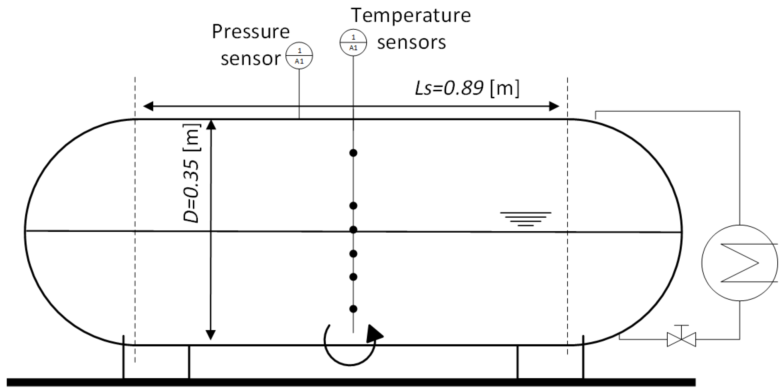
2. Experimental Work

Experiments have already been conducted in former work to study both sloshing hydrodynamics with a transparent model tank and a pressure tank made of steel to investigate the thermodynamic response. Both tanks have the same geometry. Two experiments were needed because the sloshing can not be observed with the steel tank. Figure 2 shows the experimental set-up for the thermal tank tests. The tank geometry and dimensions are the same.

The experimental rig consists of a movable platform with one degree of freedom. The tank rotates around the bottom centerplane of the tank in all tests, and the angle amplitude is equal to three degrees. The motion is created by an electro motor and a crank mechanism. As the crank arm is long compared to the radius, $L_s>>R$, the angle of the platform is approximately $\theta \left(t\right)\approx A·sin\left(2\pi f·t\right)$, where A is the amplitude, f the frequency and t is time. Several fillings and frequencies have been tested with the transparent tank to investigate sloshing characteristics. The thermal test was conducted with one filling and several frequencies. The hydrodynamic tests were conducted with water (and air), while the thermal tank tests with a mixture of liquid water and vapour and minor air content. The fact that a water/air mixture at room temperature is compared to a water liquid/vapor mixture close to the boiling point might be considered slightly controversial. The liquid density is almost unchanged, and ${\rho }_L/{\rho }_{L,max}$ varies between 1 and 0.95 at a temperature 10 and 120 ${}^{\circ }$C, respectively. Another issue is the density ratio between the gas and the liquid in each case. Maillard and Brosset [22] presented experimental studies on the influence of the density ratio between liquid and gas considering also volatile conditions. This was found to have an impact on the exchange of momentum between liquid and gas.

The density relationship between the ambient air (in the transparent case) and the vapour is given in Figure 3. It can be seen that the ratio is approximately equal at 120 ${}^{\circ }$C. The gas temperature may be as high as 135 ${}^{\circ }$C so the density ratio is not very different.

Table 1. Sloshing test conditions.

Case No.	$\mathit{h}/\mathit{D}$	$\mathit{h}/{\mathit{L}}_{\mathit{s}}$	$\mathit{f}\left(\mathit{Hz}\right)$	${\mathit{RPM}}_{\mathit{m}}$	$\mathit{f}/{\mathit{f}}_{\mathbf{1},\mathbf{0}}$	${\mathit{t}}_{\mathit{s}}/\mathit{T}$	Description
0	0.50	0.190	N/A	N/A	N/A	N/A	No motion
1	0.50	0.190	0.29	857	0.427	40	Small deformation
2	0.50	0.190	0.40	1200	0.495	31	Oscillating waves
3	0.50	0.190	0.57	1714	0.840	30	Jet formed

lists the conditions that are considered in this paper. h is the mean filling depth and D is the diameter. $L_s\left(\mathrm{m}\right)$ is the straight length of the cylindrical section, $f\left(\mathrm{Hz}\right)$ is the excitation frequency and $f_{1,0}$ is the first mode natural frequency calculated for a rectangular tank with the same length as the straight cylindrical section. $RP{M}_m$ is the rotational speed of the electro motor, $t_s$ (s) is the sloshing time and T is the motion period equal to $1/f$, such that $t_s/T$ is the number of sloshing cycles. In case 0, there is no motion and it acts as a reference condition. In case 1, there are only small deformations of the free surface. In case 2, many interacting waves are present and rapid oscillations of the free surface take place. In the last case 3, a liquid jet is found due to the spherical heads. The motion is severe in the last case and breaks up the liquid surface. These characteristics are presented later in the results.

Hydrodynamic tests have been performed to know which frequencies should be investigated in the thermal tank test. The free-surface elevation was measured with an ultrasonic sensor, model Sick UM12 (Sick Inc., Minneapolis, MN, USA). The accuracy of this sensor is $\pm 1\%$ with a repeatability of $\pm 0.15\%$. It was mounted on the top of the straight cylindrical section on the transparent tank. Videos of all the sloshing tests are recorded, using a GoPro Hero4 camera (GoPro Inc., San Mateo, CA, USA). The free-surface elevation was only possible to measure in tests with low filling because the sensor does not work in contact with water. This disadvantage should be improved in future studies.

Experiments to study the thermodynamic response due to sloshing was performed with an insulated cylindrical pressure tank made of steel. It consists of instrumentation like a pressure sensor and several thermocouples placed vertically in the middle of the tank, as seen in Figure 2. A variant of a pressure build-up unit (PBU) has been installed on the right side of the tank. It consists of a copper element heated with external voltage supply. The heater is placed lower than the mean depth, and the flow is driven by hydrostatic pressure differences. The relationship between mass flux and power supply is measured in advance to know the amount of vapour.

The test procedure consists of initial heating of the liquid from approximately 15–20 ${}^{\circ }$C to 118–119 ${}^{\circ }$C. The liquid temperature must be high to prevent any air content, and $T_{sat}-T_L$ does not get too large. The PBU power to generate vapour has been limited to 1460 W in these tests. To build up the system temperature, it can be switched between pressurisation with the heater and sloshing. The thermal energy is then mixed more efficiently inside the tank. When the system is ready for sloshing tests, the pressure is increased to the desired value. The heater is turned off and the electro-motor starts with a specified frequency and number of periods.

3. Mathematical Models and Numerical Methods

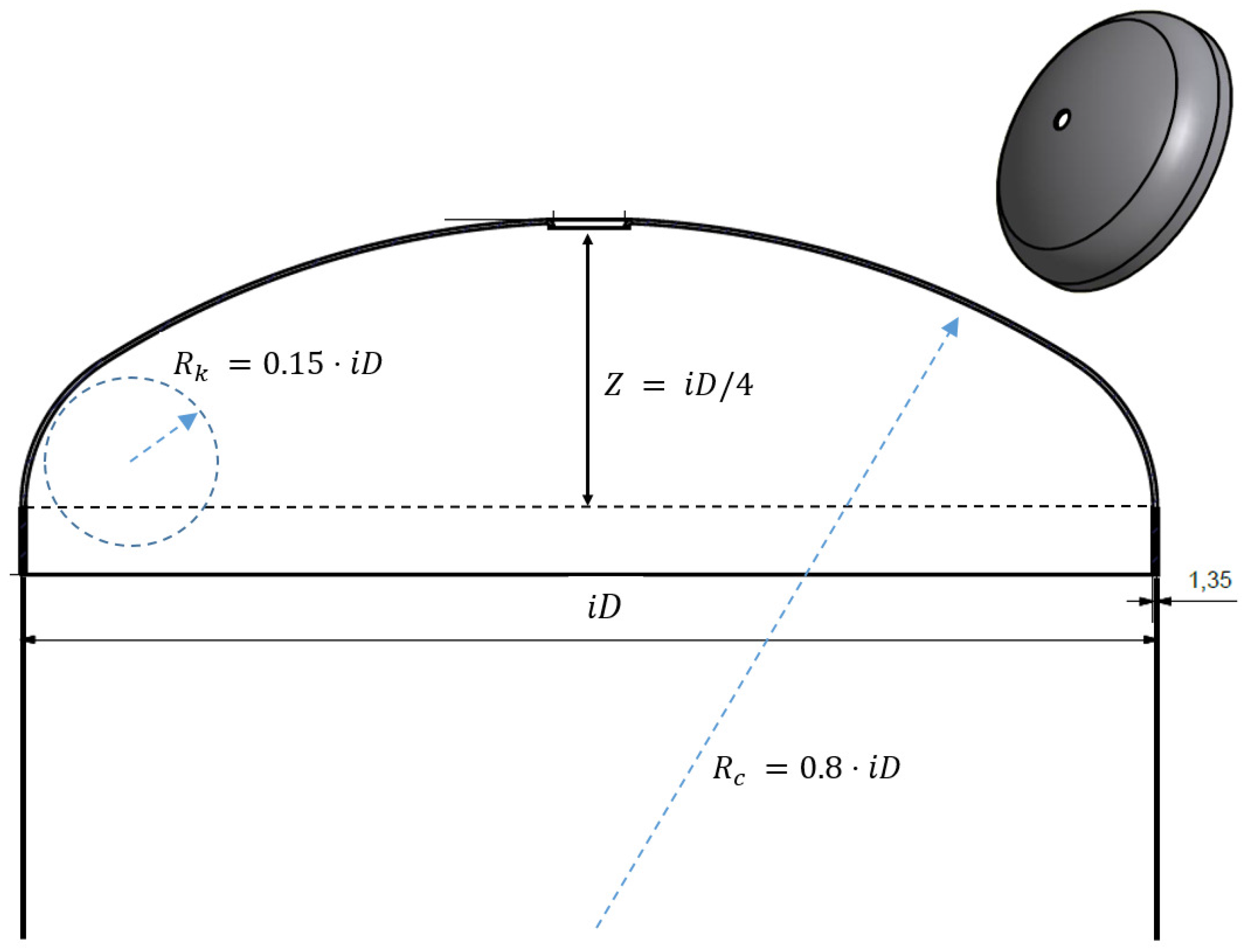
3.1. Problem Description

Numerical simulations have been performed with OpenFOAM (version 1606+, OpenCFD, London, UK). The fluid domain consists of the inner tank with the same geometry as tested in the experiments (Figure 2). Figure 4 shows the definition of the semi-elliptic heads. The crown radius, $R_k,$ and the pull-out length of the head, Z, are all scaled according to the inner diameter, which is $0.3473m$. Both tank heads are connected to a straight cylindrical section in the middle with the length $L_s=0.89m$.

The 3D geometry was constructed with the CAD tool Siemens NX (version 11.0, Siemens PLM Software, Plano, TX, USA). To generate the 3D grid, the tank geometry was exported as a .stl file. The snappyHexMesh tool in OpenFOAM is capable of reading this file format. A rectangular mesh was first generated with the blockMesh command, and then the final geometry by the use of snappyHexMesh. No additional mesh refinement has been done along the walls, but the no-slip wall boundary condition was employed on the whole surface of the tank.

This is a time-dependent problem and there is no tank motion initially. Convergence of the solving process is therefore less dependent on the initial conditions. There is no velocity in the tank and all motion-related variables are set to zero. What is important to specify is the volume of fraction of liquid and the temperature. The first one is executed by using the setFields functionality in OpenFOAM. Choosing the mean depth as a starting point is easily done with the boxToCell method. The starting temperature profile is the same as found in the experiments. The vertical profile is shown in Figure 5. The gas and liquid properties are kept constant, and the mixture density and viscosity varies with $\alpha$. The temperature is read as a non-uniform list.

The individual fluid properties of liquid and gas is kept constant and only varied by the volume fraction of liquid. The specific enthalpy of formation is kept constant and equal to $2.257\times {10}^6[\mathrm{J}/\mathrm{kg}]$. The values are given in

Table 2. Fluid properties.

Phase	$\mathit{\rho }(\mathbf{kg}/{\mathbf{m}}^3)$	$\mathit{\nu }({\mathbf{m}}^{\mathbf{2}}/\mathbf{s})$	${\mathit{c}}_{\mathit{p}}(\mathbf{J}/\mathbf{kg}·\mathbf{K})$	$\mathit{k}(\mathbf{W}/\mathbf{m}·\mathbf{K})$
Liquid	997.56	$8.91\times {10}^{-7}$	4180	0.62
Gas	1.18	$1.57\times {10}^{-5}$	1500	0.03

.

3.2. CFD-Model

It is assumed that the flow is incompressible, such that

$$\mathsf{\nabla }·\mathbf{v}=0,$$

(1)

where $\mathbf{v}$ is the mean velocity vector.

The Reynolds-averaged Navier–Stokes equations (RANS) are solved numerically with a pressure-correction algorithm. The equation is written in tensor notation as [23]

$$\frac{\partial }{\partial t}\left(\rho \mathbf{v}\right)+\mathsf{\nabla }·\left(\rho \mathbf{v}\mathbf{v}\right)=-\mathsf{\nabla }p+\mathsf{\nabla }·\left\{\left(\mu +{\mu }_t\right)\left[\mathsf{\nabla }\mathbf{v}+{\left(\mathsf{\nabla }\mathbf{v}\right)}^{\mathrm{T}}\right]\right\}+{\mathbf{f}}_b.$$

(2)

$\rho$ is the density, p is the pressure, $\mu$ the dynamic molecular viscosity and ${\mathbf{f}}_b$ are external forces like gravity.

To account for turbulence, the Boussinesq-concept is employed, where turbulence affects the mean velocity field as additional viscosity. The turbulent dynamic viscosity, ${\mu }_t$, is estimated by the use of the $k-\omega$ SST turbulence model [24,25,26]. The model equations implemented in OpenFOAM are

$$\frac{\partial }{\partial t}\left(\rho k\right)+\mathsf{\nabla }·\left(\rho \mathbf{v}k\right)={\tilde{P}}_k-{\beta }^{*}k\omega +\mathsf{\nabla }·\left\{\left(\mu +{\sigma }_k{\mu }_t\right)\mathsf{\nabla }k\right\},$$

(3)

$$\begin{array}{c}\frac{\partial }{\partial t}\left(\rho \omega \right)+\mathsf{\nabla }·\left(\rho \mathbf{v}\omega \right)=\alpha \rho S^2-\beta \rho {\omega }^2+\mathsf{\nabla }·\left\{\left(\mu +{\sigma }_{\omega }{\mu }_t\right)\mathsf{\nabla }\omega \right\}\\ +2\left(1-F_1\right)\rho {\sigma }_{\omega 2}\frac{1}{\omega }\mathsf{\nabla }k·\mathsf{\nabla }\omega ,\end{array}$$

(4)

$${\mu }_t=\frac{\rho a_{1}k}{\mathrm{Max}\left(a_1\omega ,S{F}_2\right)},$$

(5)

$${\tilde{P}}_k=\mathrm{Min}\left(P_k,10{\beta }^{*}k\rho \omega \right);P_k={\mu }_t\mathsf{\nabla }\mathbf{v}:\left[\mathsf{\nabla }\mathbf{v}+{\left(\mathsf{\nabla }\mathbf{v}\right)}^{\mathrm{T}}\right].$$

(6)

Here, S is the magnitude of the strain rate, $F_1$ is a blending function, which is zero away from the surface ($k-ϵ$) and switches to unity inside the boundary layer ($k-\omega$). $F_2$ is the second blending function. The blended parameters are ${\sigma }_k$, ${\sigma }_{\omega }$, $\alpha$ and $\beta$. The model constants, ${\beta }^{*},{\sigma }_{k1},{\sigma }_{k2},{\sigma }_{\omega 1},{\sigma }_{\omega 2},{\alpha }_1,{\alpha }_2,{\beta }_1,{\beta }_2$ and $a_1$, all have default values, equal to 0.09, 0.85, 1.00, 0.50, 0.856, 5/9, 0.44, 3/40, 0.0828 and 0.31, respectively [26,27].

The $\omega$-equation can be integrated through the wall boundary layer, which is advantageous for the near wall treatment. OpenFOAM offers near wall treatment that can automatically switch between low and high Reynolds number formulations. The solution to this is blending between the analytical solutions of $\omega$ in the viscous sublayer and the logarithmic near-wall region [28]:

$$\omega ={\left[{\omega }_{vis}^2+{\omega }_{log}^2\right]}^{0.5},$$

(7)

$${\omega }_{vis}=\frac{6\nu }{0.075y^2};{\omega }_{log}=\frac{1}{0.3\kappa }\frac{u_{\tau }}{y},$$

(8)

where y is the normal distance from the wall face to the cell center of the nearest cell. $\kappa$ is the von Karman constant. A similar blending is performed for the velocity profile near the wall. The boundary condition for turbulence energy, k, at the wall is a zero gradient.

An additional transport equation is solved to find the volume fraction. The fluid properties in hydrodynamic applications are

$$\rho ={\alpha }_L{\rho }_L+\left(1-{\alpha }_L\right){\rho }_G,\nu ={\alpha }_L{\nu }_L+\left(1-{\alpha }_L\right){\nu }_G,$$

(9)

where ${\alpha }_L$ is the volume fraction of liquid. $\rho$ and $\nu$ is the density and kinematic viscosity, respectively. The volume fraction of liquid is transported in the domain by solving the equation

$$\frac{\partial \alpha }{\partial t}+\mathsf{\nabla }·\left(\mathbf{v}\alpha \right)+\mathsf{\nabla }·\left\{{\mathbf{v}}_{\mathrm{r}}\alpha \left(1-\alpha \right)\right\}=0.$$

(10)

The last term is an artificial compression term, where ${\mathbf{U}}_r$ is a velocity field suitable to compress the interface. It should act normal at the interface and can be based on the maximum velocity magnitude in the transition region [29]. An advantage of Equation (10) is that its solution for $\alpha$ can be bounded between 0 and 1. This is controlled by the cAlpha parameter in the fvSolution file. If equal to 1, the compression is conservative and, above 1, it is not. In this paper, the value 1.0 is used in order to obey mass conservation.

The final equilibrium state can be estimated, but the time to reach it is unknown. A method to predict the time to reach the equilibrium condition has been implemented in the existing OpenFOAM solver. The energy equation contains a source term that is activated only at the interface and is proportional to the temperature difference $\left(T-T_{sat}\right)$. The saturation temperature is taken here as the average of the gas temperature (Appendix A.1). This is reasonable because it has been observed in experiments that the saturation and the gas temperature are very close and vary parallel to each other. The pressure drop rate may thus be calculated from the corresponding saturation temperature. The main assumption is that the pressure drop rate is depending directly on the rate of cooling of the gas by the liquid. Initial temperatures found in the experiments are used in the start of the simulations by interpolating the sensor values onto the grid.

The first step is to implement a thermal transport equation in the interDyMFoam solver. The following version is used:

$$\frac{\partial \left(\rho T\right)}{\partial t}+\mathsf{\nabla }·\left(\rho \mathbf{U}T\right)=\mathsf{\nabla }·\left[\left(k_{eff}/c_p\right)\mathsf{\nabla }T\right]+{\dot{S}}_T.$$

(11)

The thermal conductivity $k_{eff}$ in Equation (11) contains the molecular conductivity as well as the contribution from turbulence, $k_t$.

${\dot{S}}_T$ is the heat source activated only at the free surface. k and $c_p$ are mixture properties found with the volume fraction, and given as

$${\alpha }_L{k}_L+(1-{\alpha }_L)k_G,$$

(12)

$${\alpha }_L{c}_{p,L}+(1-{\alpha }_L)c_{p,G}.$$

(13)

The turbulent thermal conductivity is given in a classical manner as

$$k_t=\frac{\rho c_p{\nu }_t}{P{r}_t}.$$

(14)

${\nu }_t$ is the turbulent kinematic viscosity. The turbulent Prandtl number, $P{r}_t$ needs to be taken as a constant value. Here, we have used the value equal to 2, which is slightly larger than normal. This is because turbulence is overproduced at the surface with VOF-based two-phase calculations. The implementation of Equation (11) is given in Appendix A.2.

The source term is expressed almost similar to what was done in [17,18]. The difference is that the source term is activated only at the interface. It is given as

$${\dot{S}}_T=r\rho 2{\alpha }_L\left(1-{\alpha }_L\right)\frac{T-T_{sat}}{T_{sat}}{h}_{fg}/c_p.$$

(15)

r is a constant equal to 0.1 s${}^{-1}$. The term $2{\alpha }_L\left(1-{\alpha }_L\right)$ is a harmonic mean value of the liquid volume fraction. It is zero everywhere else than at the interface. It ensures a smooth transition between the phases. The saturation temperature is updated each time step. A prerequisite for this assumption is that the thermal energy in the gas relative to saturated conditions is negligible compared to the liquid. The pressure is estimated from the saturation temperature, $P\left(T_{sat}\right)$. This is done by the use of Tetens equation [30],

$$P_{sat}=0.61078·exp\left(\frac{17.27T}{T+237.3}\right).$$

(16)

The units of pressure P and temperature T are kPa and ${}^{\circ }\mathrm{C},$ respectively.

3.3. OpenFOAM Solver InterDyMFoam

InterDyMFoam is a solver for two incompressible, isothermal immiscible fluids with optional mesh motion and mesh topology changes including adaptive re-meshing. This is ideally suited for sloshing. Mesh refinement is not performed, only motion of the whole mesh. The VOF method is used to capture the location of the interface, which determines the cells that contain gas or liquid properties.

The rotational amplitude and frequency is given in a tabulated file read by OpenFOAM. The rotational point was specified to be the same as in the experiments, as in Figure 2.

Although OpenFOAM offers a semi-implicit version of MULES [31], the maximum Courant number is limited to 0.5 in all the simulations. This ensures a small time step. When the time step is small, the pressure-velocity coupling is stronger than the nonlinear convective momentum term. It is therefore not necessary to update the velocity more than once per time step. This is essentially the Pressure-Implicit with Splitting of Operators (PISO) algorithm [32] and is chosen in OpenFOAM by setting the nOuterCorrectors to 1, and performing several pressure corrections, typically 3. PISO is efficient, and the accuracy is good with the strict Courant number limit. A drawback to PISO is that it is found to be more sensitive to the mesh.

The pressure-velocity coupling is traditionally dealt with using a staggered-grid technique. However, it becomes an issue on non-Cartesian and unstructured grids. In OpenFOAM, a variant of the Rhie and Chow interpolation technique [33] is used, which offers the possibility of formulating the PISO algorithm on a collocated grid. The Rhie–Chow interpolation is different in OpenFOAM, and a summary can be found in [34].

4. Results

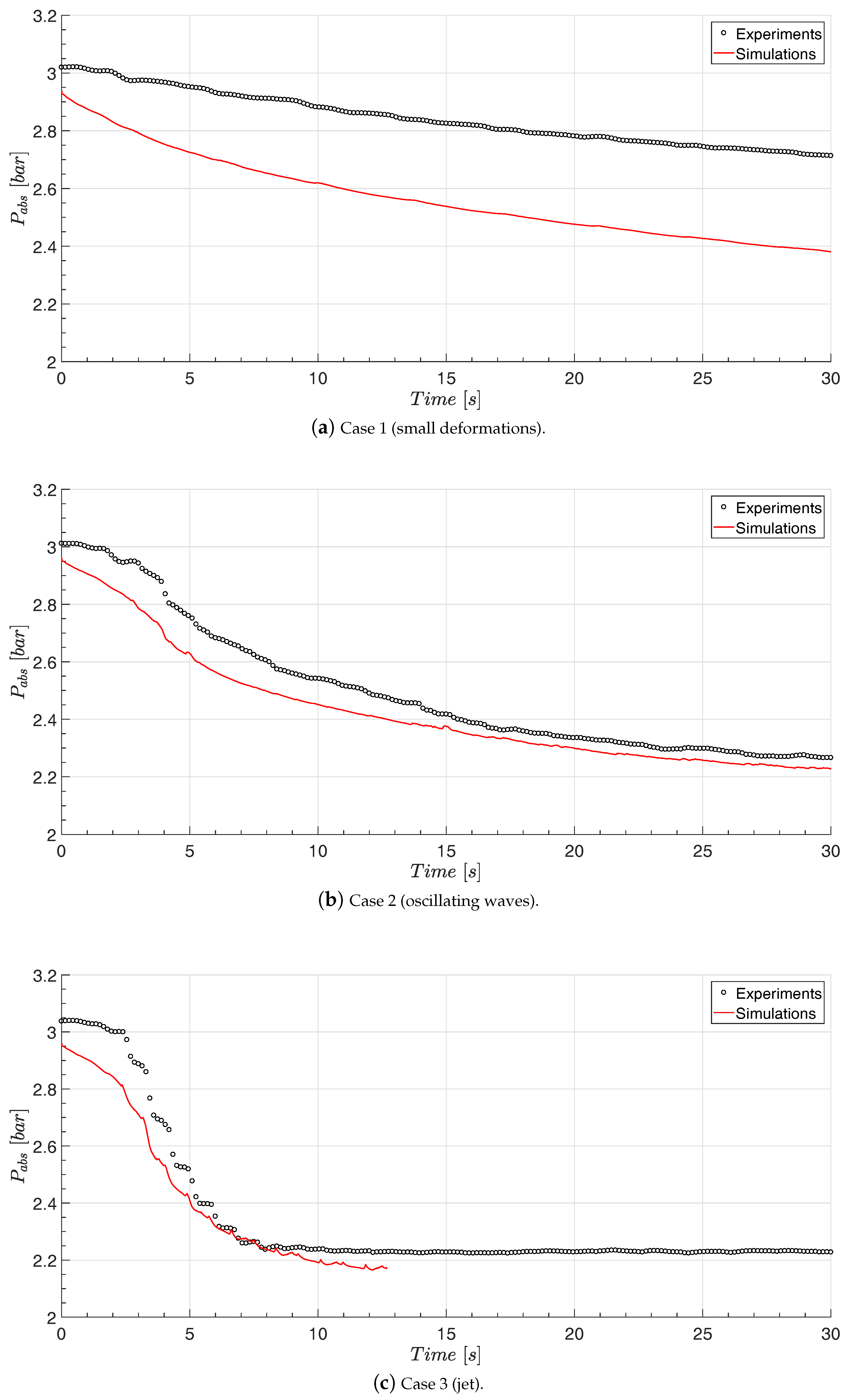
4.1. Experiments—Thermodynamic Response with Water

The pressure from the thermal tests are compared in Figure 6. Observations from the hydrodynamic tests are are also added to show the sloshing conditions. It can be seen that, during this time of sloshing, only cases 2 and 3 have enough intensity to reach the equilibrium condition. The pressure development is quite different in all of the cases, where the most rapid pressure drop occurs in case 3. The results are similar to what was found in [6], and the most rapid pressure collapse is found when the sloshing is severe and close to the primary resonance, $f/f_{1,0}=1$. The rise in pressure seen after the minimum in case 3 happens because the liquid now is saturated and starts to evaporate. The only dominant energy source is now the heat ingress, as the liquid is no longer subcooled. The sudden stop in the pressure drop was also mentioned by Ludwig et al. [10], but the rise in pressure is only possible with heat ingress.

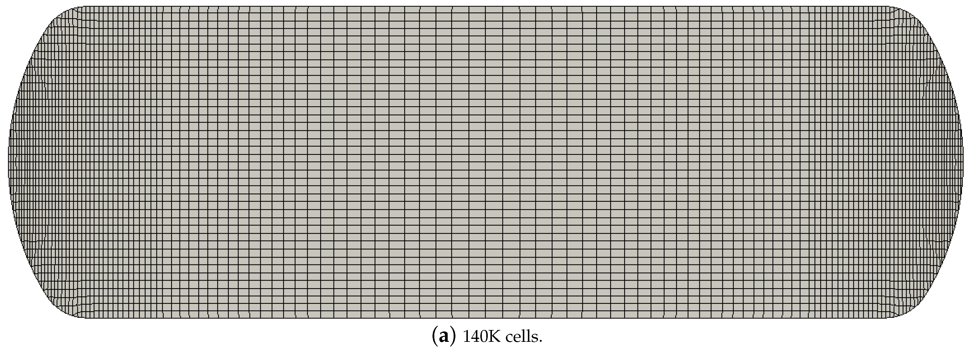
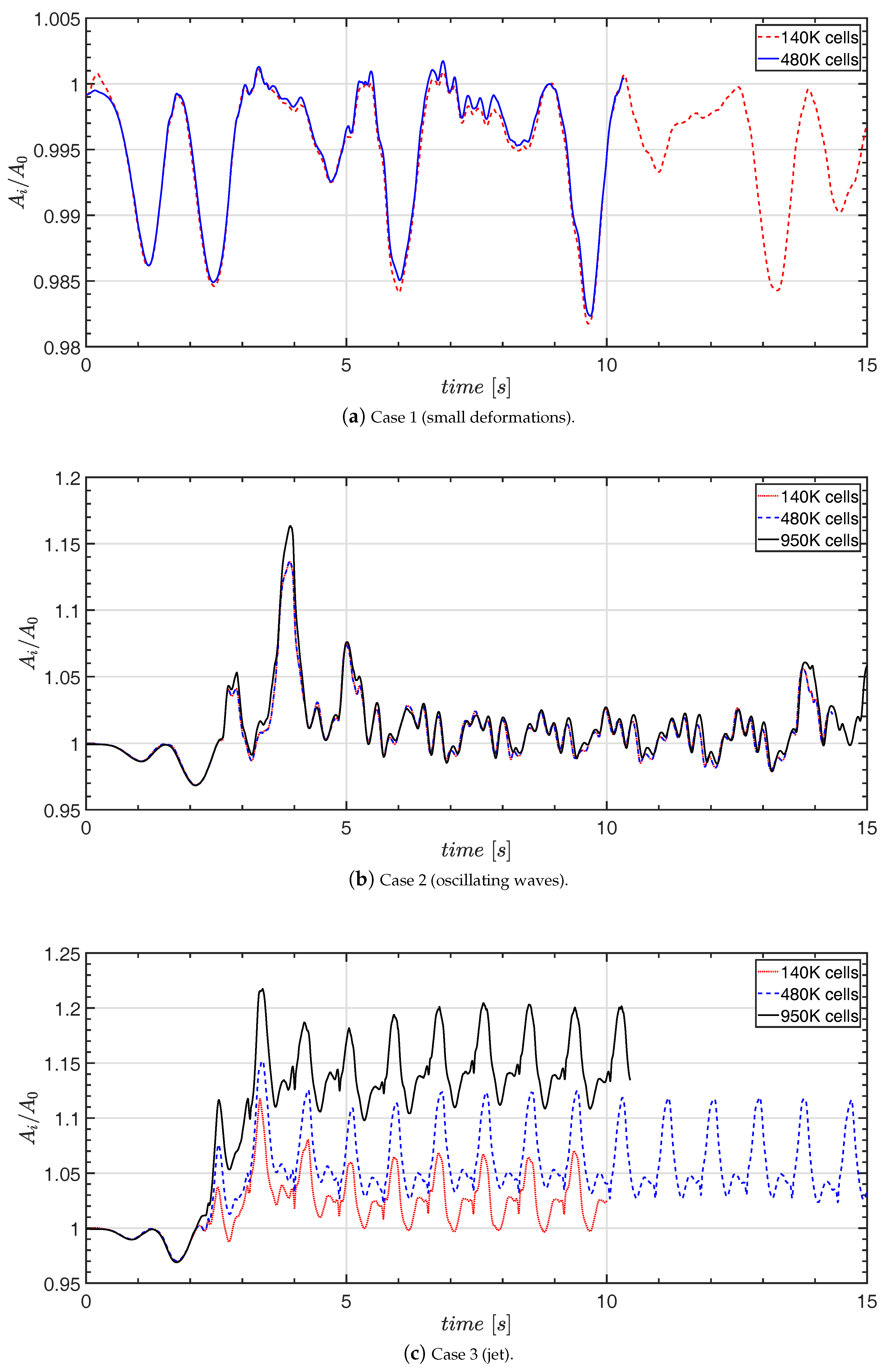
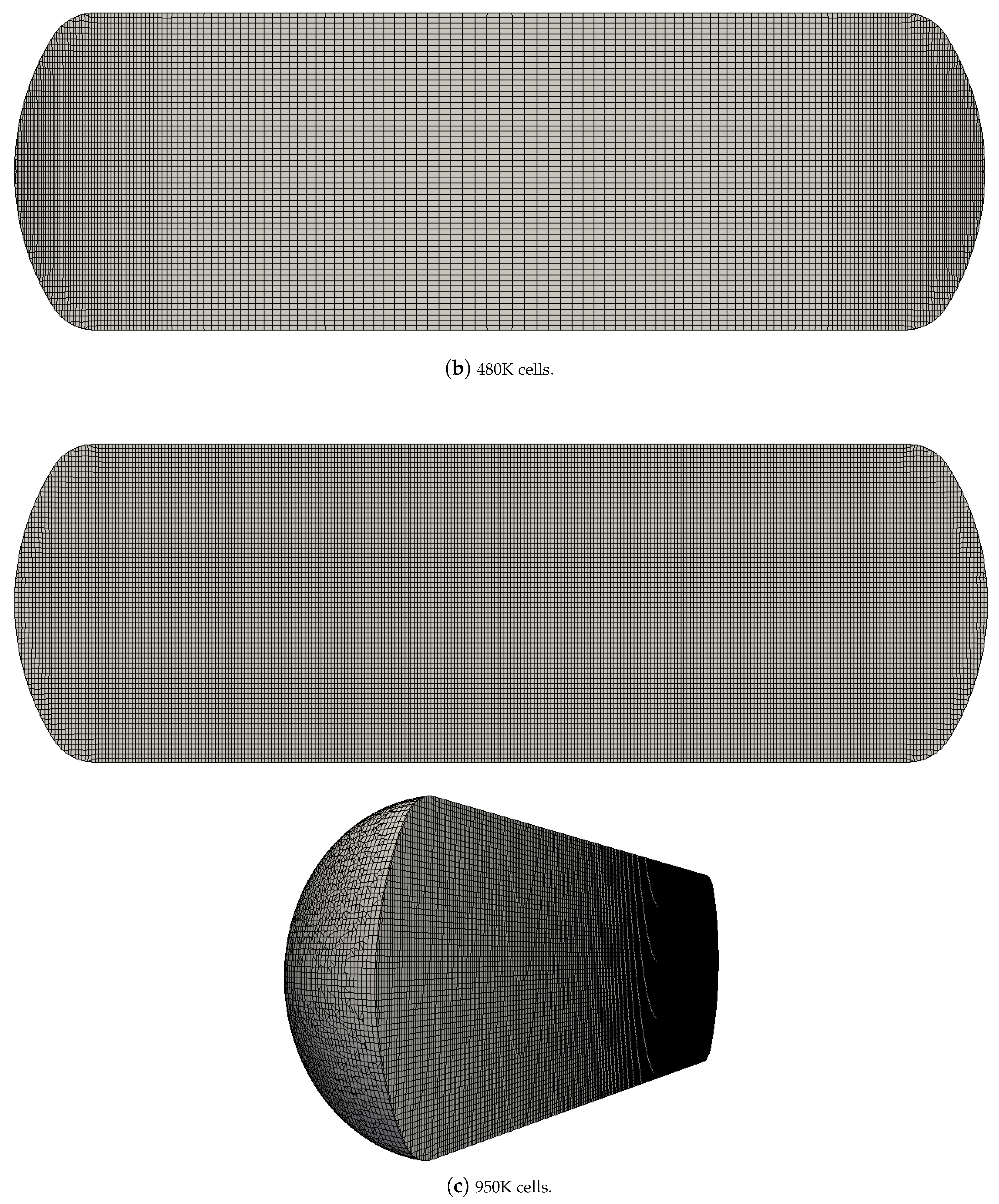
4.2. Grid Independence Study

Three different grid resolutions have been compared by simulating sloshing hydrodynamics and calculating the interface area for all the cases in Table 1. The no-motion case is also simulated, but only with the coarsest grid. The three grids are presented in Figure 7. The two coarsest grids, (Figure 7a,b are slightly stretched horizontally towards each tank head.

The interface area is supposed as important for the energy exchange between liquid and gas. It is difficult, if not impossible, to obtain it from experiments. To some extent, this is possible with CFD. The area prediction naturally depends on the grid refinement. A way to estimate such unknown variables is to perform a grid-independence study. This does not require us to compare with experimental data.

Cases 1–3 in Table 1 have been simulated on all three grids. Simulations have been performed computing on 40 nodes on the high-performance computing (HPC) cluster “Stallo” [35]. Some additional code was added directly into the interDyMFoam solver to obtain the area at each time step. The code is given in Appendix A.3. The code basically creates a volume field that equals the magnitude of the volume fraction gradient. The gradient is then integrated all over the domain.

The result is shown in Figure 8. Convergence is not achieved in the most severe sloshing case 3. Although some splashing is found in case 2, the free surface remains continuous most of the time. The jet is thus difficult to resolve with the grid. However, it is not only the peaks that occur every half a period that deviates. The time-averaged surface area is also quite different with each grid. The interface area is larger in case 3 than 1 and 2. However, the percentage increase of the area in cases 2 and 3 seems to be less than expected. The mean surface area in case 3 is approximately 15% larger compared to the undisturbed case for the finest grid.

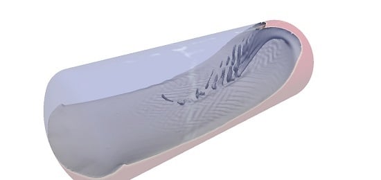
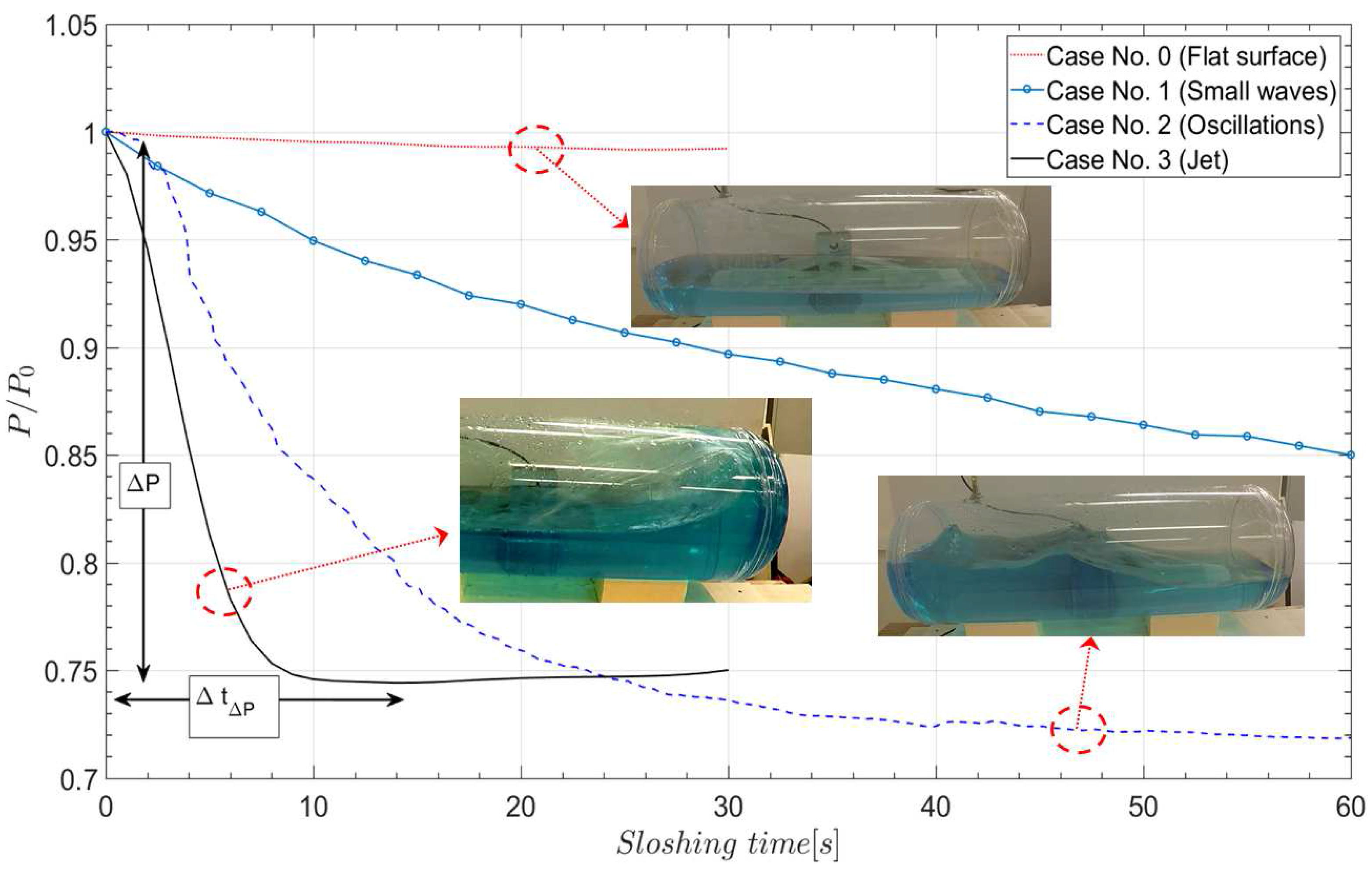
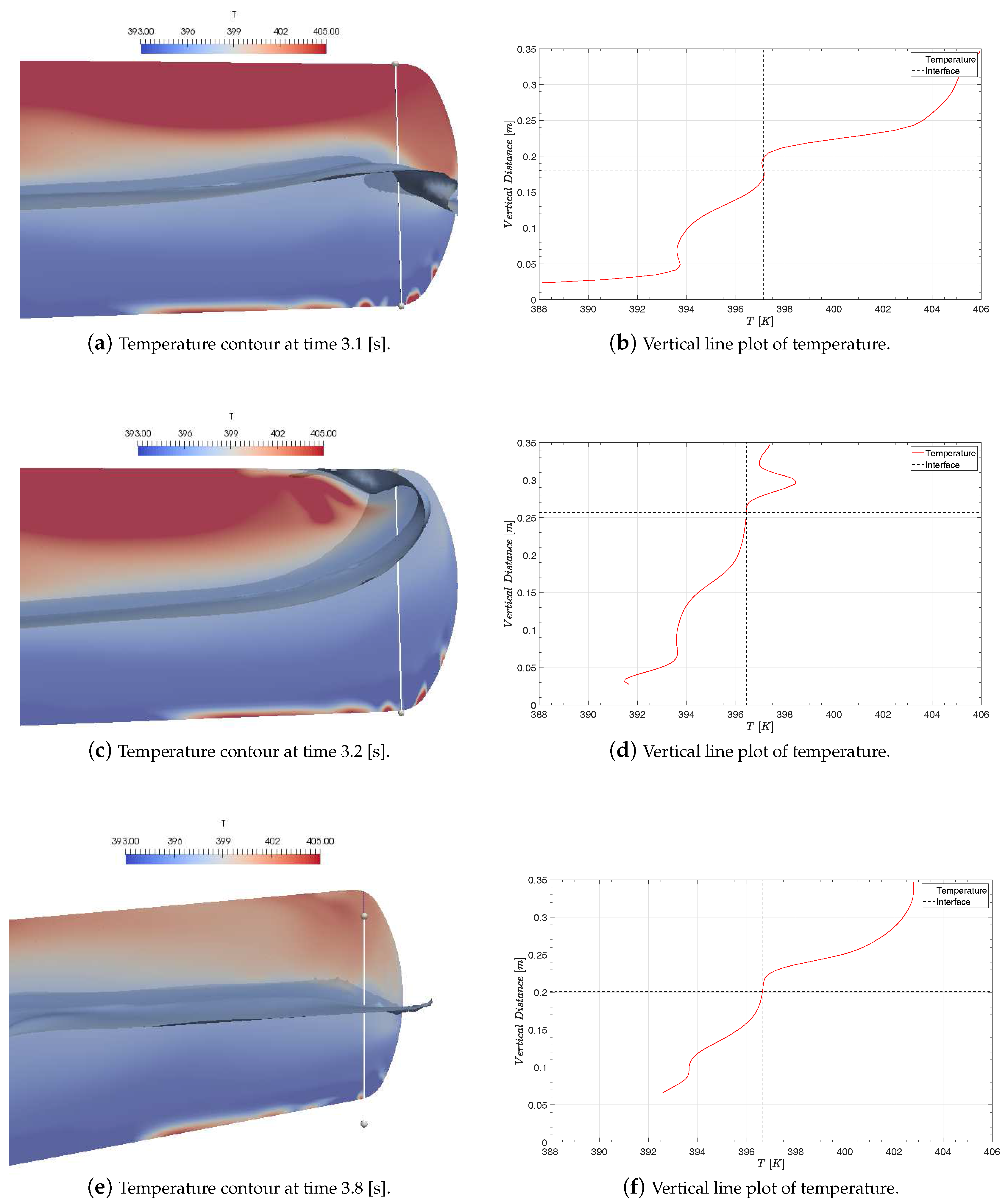
4.3. The Influence of the Liquid Jet

By taking a closer look at the pressure measurements from experiments in case 3 (Figure 9), one can see that the pressure consists of smaller periodic oscillations. This is most pronounced for case 3, but can be seen also in the other cases.

The mass condensation rate is proportional to $-dP/dt$, which can be calculated numerically from the measurements. Assuming that the gas volume is constant, and differentiating the ideal gas law, $pV=mRT$ gives:

$$\frac{dP}{dt}=-\frac{P}{m_G}\frac{d{m}_L}{dt}+\frac{P}{T_G}\frac{d{T}_G}{dt},$$

(17)

where $m_G$ is the mass of gas, $T_G$ is the gas temperature and $m_L$ is the mass of the liquid. It has been found by sensitivity studies that the change in gas temperature has a minor influence on the pressure because the gas temperature is nearly saturated. Hence, the last term may be excluded.

The area found from the CFD calculations can be compared to the mass rate of change by normalizing the values and plot over time. The result is shown in Figure 10. The calculated maximum area from CFD is in phase with the maximum values of the mass condensation rate. Only a small phase shift is found in the beginning. As the temperature in proximity to the liquid surface raises, the condensation ceases. It is not sure whether the area increase itself is the only important factor here. From the figures, it is also observed that the jet impacts the surface at the time of the peak values. Another factor that might be important is the transport of cold liquid from the bulk, which is done efficiently with the jet. It also enhances the mixing between liquid and gas, as the gas is trapped between the jet and the liquid surface.

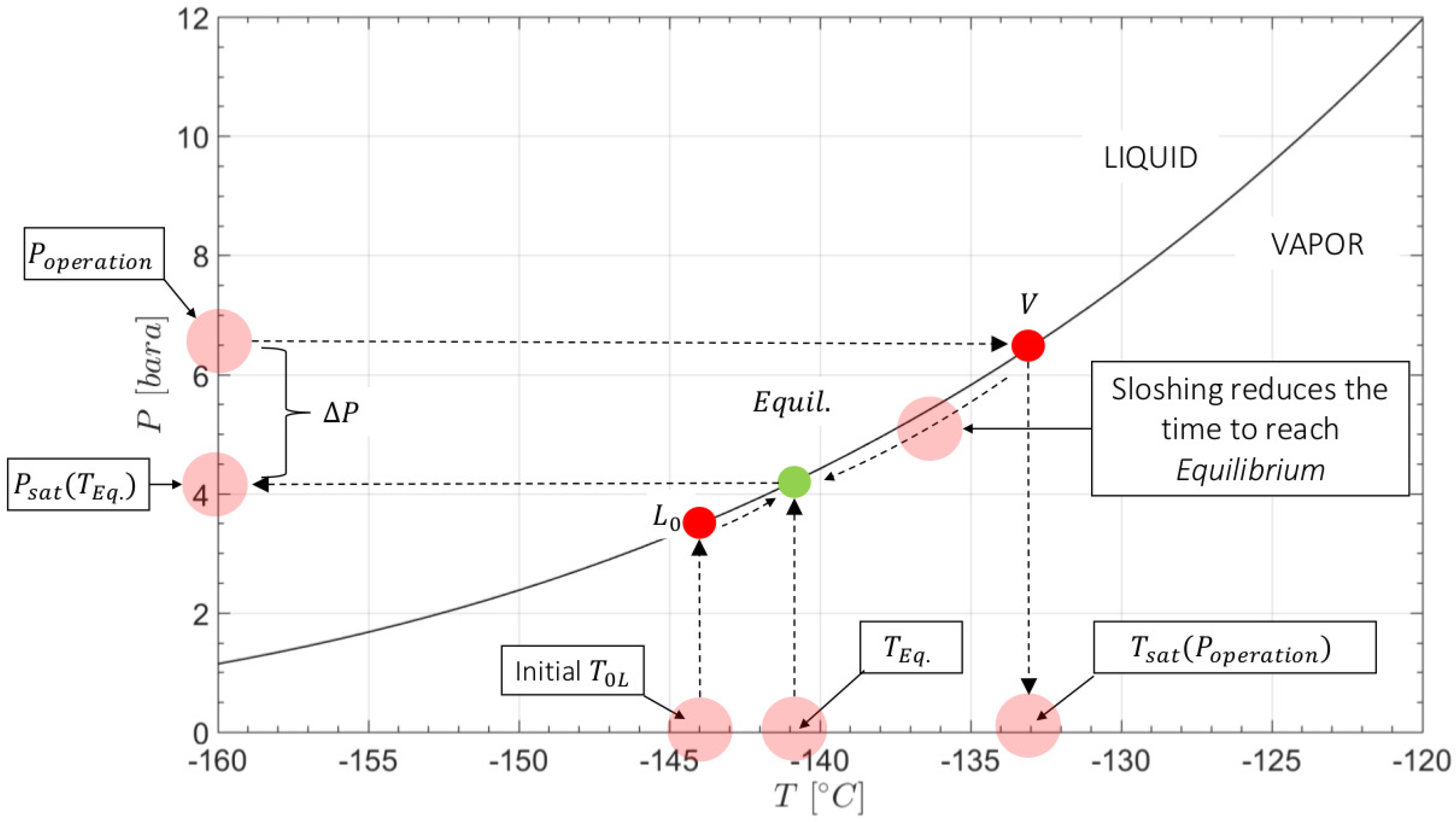
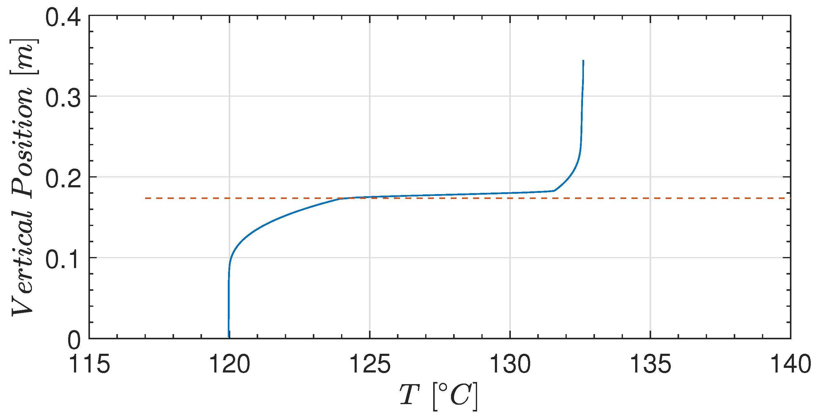
4.4. Prediction of Pressure and Temperature

Cases 0–3 have been simulated using the finest grid with $951\times {10}^3$ cells (Figure 7c). Figure 11 shows the comparison of pressure between CFD and experiments. The agreement is good in cases 2 and 3 (Figure 11b,c), while, in case 1 (Figure 11a), the pressure drop is over-predicted in the analysis. The discrepancy in case 1 may be explained by the fact that the temperature field is diffusive across the gas–liquid interface. Cases with severe sloshing may depend less on this unrealistic diffusion because the turbulence is much more pronounced and "camouflage" the error. This conclusion would require more in-depth studies. As may be observed, the pressure from CFD is slightly lower than the experiments in all cases. The reason is that the actual saturation temperature is slightly higher than the weighted average gas temperature. A prerequisite for the model to be realistic is that the gas is nearly saturated. The difference is irrelevant as the curves are parallel to each other, and the agreement is overall good.

Some plots of the temperature development in the tank are shown in Figure 12. In the column of figures to the left, contour plots of temperature are presented. The white line shows where the vertical profile at the right is plotted inside the tank. The first two Figure 12a,b is showing the wave just in an instant before the jet is formed along the wall. This is early in the sloshing event, and the temperature gradient is steep on both sides.

In the next two pairs of figures, the water hits the roof and the temperature profile is much more uniform. It is seen that the temperature above the interface is close to the initial interface temperature. The jet thus transports cold liquid quite efficiently towards the liquid surface.

In the last figure, the wave is heading towards the opposite end, and the the cooling of the gas is clearly visible from the first time (Figure 12b) to the last (Figure 12f). The gas bulk temperature has dropped four degrees during these few seconds. The results may explain why the pressure is dropping so efficiently close to resonance. The surface area might not be the dominating factor, but rather the transport of liquid bulk towards the surface. The jet enhances the mixing between liquid and gas quite efficiently.

5. Discussion

Although the accuracy of the calculated interface area is quite uncertain for the jet case, the overall impression is that the area has less influence than what was expected. Case 2, which has a moderate pressure drop rate, and for which the area seems to be accurately determined, shows just a minor increase. However, it is pronounced in the beginning, while it ceases after a few seconds. The correspondence between the jet and the mass condensation rate given in Figure 10 still indicates that the area might be responsible for the large pressure drop. Another factor that is likely to be important is the transportation of cold bulk onto the interface area that takes place in a jet event. This was found to be important as shown in the last part of the previous section. If this is the case, it is understandable why the resonant cases results in the enhanced thermal response. It tells us that breaking waves results in rapid loss of pressure.

To estimate the maximum area expected in sloshing, an exercise is performed where the surface area of a liquid drop of a certain diameter equivalent to a percentage liquid volume is calculated. The result in

Table 3. Surface area for a number of liquid drops of 1 [cm] diameter equivalent to a percentage of the total liquid volume in the tank. Space between the drops are excluded. The undisturbed surface area is the same as in the large tank, equal to $A_0=0.365$ ${\mathrm{m}}^2$.

% Liquid Volume	Volume [L]	N Drops	Surface Area (${\mathbf{m}}^{\mathbf{2}}$) Drops	${\mathit{A}}_{\mathit{i}}/{\mathit{A}}_{\mathbf{0}}$
1.0	0.48	907	0.29	0.78
2.5	1.19	2268	0.71	1.95
5.0	2.38	4536	1.43	3.90
10.0	4.75	9072	2.85	7.81
15.0	7.13	13,608	4.28	11.71
20.0	9.50	18,144	5.70	15.62

give the overall surface area if 10% of the total liquid volume contains the equivalent number of particles of a specified diameter of 1 cm.

The estimated area from CFD is uncertain in case 3 where drops may be expected, and the area may be much greater as seen from Table 3. The free surface in case 2 does not break. It is therefore difficult to tell from the calculated area value if this has a significant effect on heat transfer or not. It is most likely to be a combination of the local heat transfer mechanisms and the bulk mixing. Both are contributing, but the time scales are quite different.

6. Conclusions

Numerical simulations of sloshing both considering sloshing hydrodynamics as well as thermal mixing have been performed. The tool used is OpenFOAM, and an existing solver was modified to include a transport equation for thermal energy. Simulations with three different excitation frequencies have been performed with 50% filling in the tank. The interface area was calculated with three different grids and compared. Comparison was also made between the calculations and experimental results. The pressure drop from simulations was compared to experimental results in the last part of the paper. The thermal mixing was studied as well.

The following conclusions can be made considering the aforementioned studies:

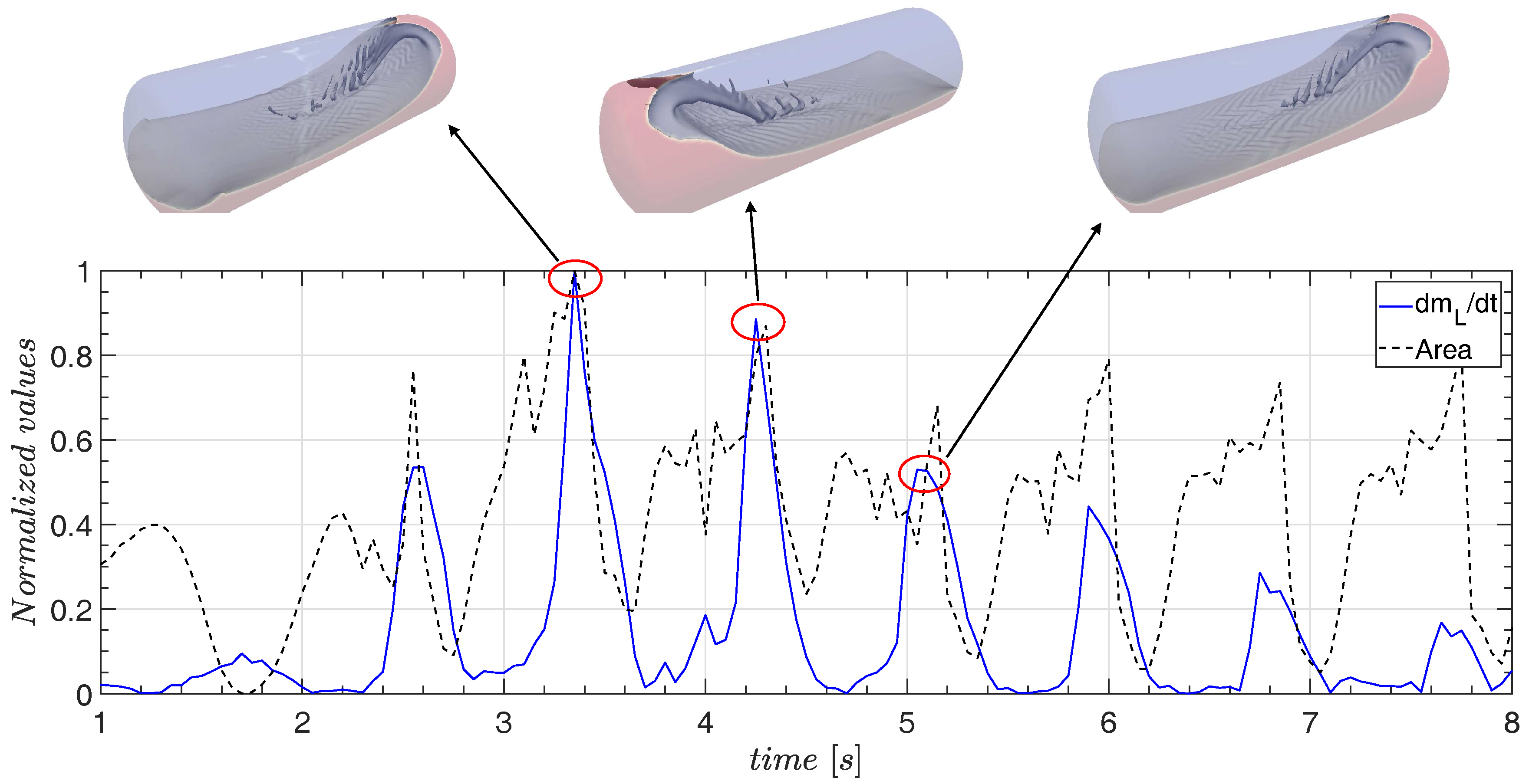
• The grid independence study indicates that the area can be estimated when the free surface does not break. Grid convergence was not found in case 3.
• The increase of the interface area is approximately 2.5% in case 2 when the sloshing is closer to a quasi-steady condition.
• The interface area is not accurately determined in case 3, but the results indicate that the area is larger than in case 2, but may be less than an increase of 50% relative to the undisturbed area.
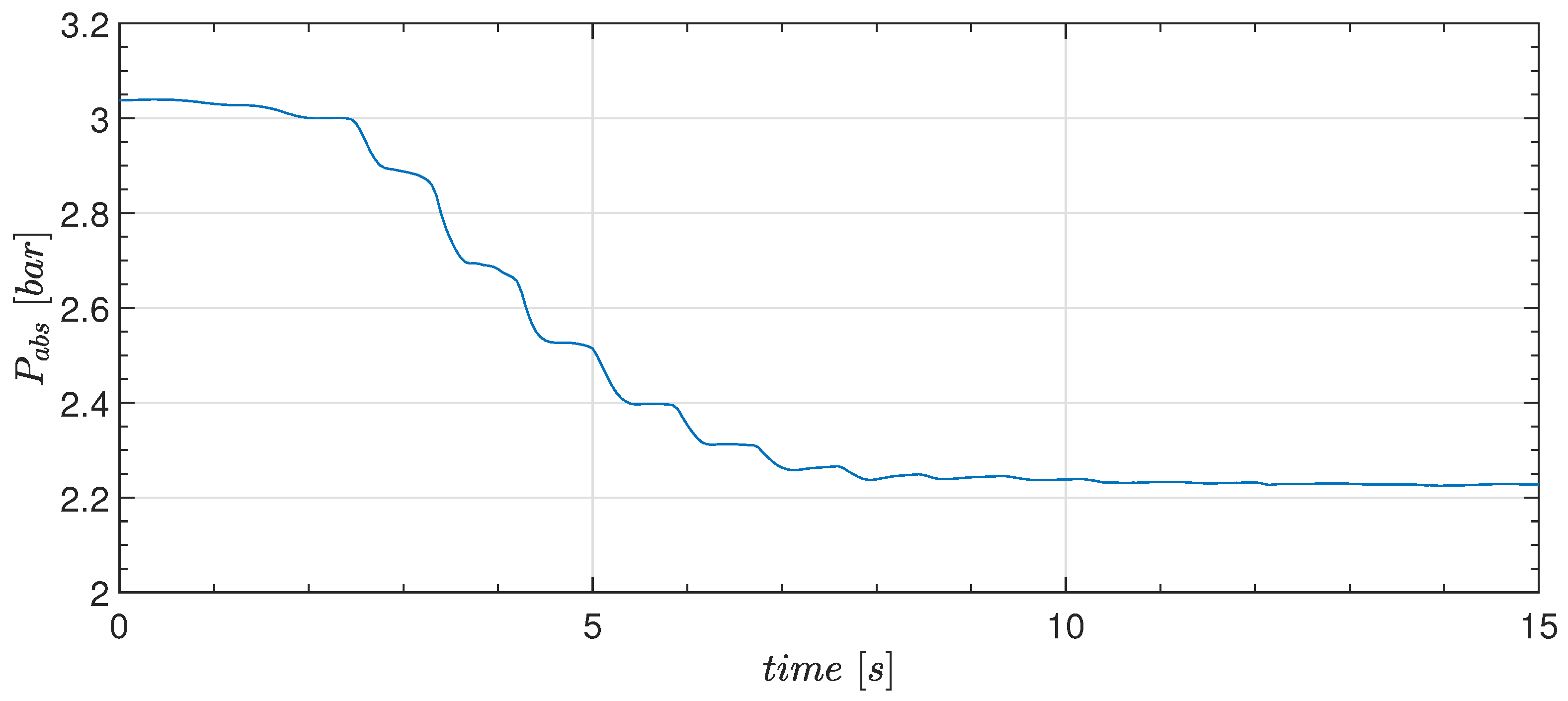
• The pressure measurement in case 3 shows correspondence with the sloshing hydrodynamics, and the occurrence of the jet clearly influences the pressure drop.
• Results from simulations with the extended OpenFOAM solver shows acceptable agreement with the measured pressure, and may be used for further investigation. However, it is quite uncertain to what extent the model is applicable for other cases with other components, initial conditions, etc.

Further work must be conducted where the area is calculated with grids of different resolution. Comparison with experimental data should be investigated. The CFD model shows potential, but must be improved further. More detailed development work on CFD and direct-contact heat transfer problems should also be done.

References

1. Æsøy, V.; Stenersen, D. Low emission LNG fuelled ships for environmental friendly operations in arctic areas. In Proceedings of the ASME 2013 32nd International Conference on Ocean, Offshore and Arctic Engineering, Nantes, France, 9–14 June 2013; p. V006T07A028. [Google Scholar]
2. Faltinsen, O.M.; Timokha, A.N. Sloshing; Cambridge University Press: Cambridge, UK, 2009. [Google Scholar]
3. Æsøy, V.; Einang, P.M.; Stenersen, D.; Hennie, E.; Valberg, I. LNG-fuelled engines and fuel systems for medium-speed engines in maritime applications. SAE Tech. Paper 2011. [Google Scholar] [CrossRef]
4. Grotle, E.; Æsøy, V.; Pedersen, E. Modelling of LNG fuel systems for simulations of transient operations. In Maritime-Port Technology and Development; CRC Press: Cleveland, OH, USA, 2014; p. 205. [Google Scholar]
5. Lemmon, E.W.; Huber, M.L.; McLinden, M.O. NIST Standard Reference Database 23: Reference Fluid Thermodynamic and Transport Properties-REFPROP; version 9.1; National Institute of Standards and Technology: Gaithersburg, MD, USA, 2013.
6. Grotle, E.L.; Halse, K.H.; Pedersen, E.; Li, Y. Non-Isothermal Sloshing in Marine Liquefied Natural Gas Fuel Tanks. In Proceedings of the 26th International Ocean and Polar Engineering Conference, Rhodes, Greece, 26 June–1 July 2016; International Society of Offshore and Polar Engineers: Mountain View, CA, USA, 2016. [Google Scholar]
7. Moran, M.E.; Mcnelis, N.B.; Kudlac, M.T.; Haberbusch, M.S.; Satornino, G.A. Experimental results of hydrogen slosh in a 62 cubic foot (1750 liter) tank. In Proceedings of the 30th Joint Propulsion Conference, Indianapolis, IN, USA, 27–29 June 1994. [Google Scholar]
8. Lacapere, J.; Vieille, B.; Legrand, B. Experimental and numerical results of sloshing with cryogenic fluids. Progress in Propulsion Physics. EDP Sci. 2009, 1, 267–278. [Google Scholar]
9. Arndt, T. Sloshing of Cryogenic Liquids in a Cylindrical Tank under Normal Gravity Conditions; Universtität Bremen: Bremen, Germany, 2011. [Google Scholar]
10. Ludwig, C.; Dreyer, M.; Hopfinger, E. Pressure variations in a cryogenic liquid storage tank subjected to periodic excitations. Int. J. Heat Mass Transf. 2013, 66, 223–234. [Google Scholar] [CrossRef]
11. Lin, C.S.; Hasan, M.; Nyland, T. Mixing and transient interface condensation of a liquid hydrogen tank. In Proceedings of the 29th Joint Propulsion Conference and Exhibit, Monterey, CA, USA, 28–30 June 1993. [Google Scholar]
12. Juric, D.; Tryggvason, G. Computations of boiling flows. Int. J. Multiph. Flow 1998, 24, 387–410. [Google Scholar] [CrossRef]
13. Welch, S.W.; Wilson, J. A volume of fluid based method for fluid flows with phase change. J. Comput. Phys. 2000, 160, 662–682. [Google Scholar] [CrossRef]
14. Youngs, D.L. Time-dependent multi-material flow with large fluid distortion. In Numerical Methods for Fluid Dynamics; Academic Press: Cambridge, MA, USA, 1982. [Google Scholar]
15. Hardt, S.; Wondra, F. Evaporation model for interfacial flows based on a continuum-field representation of the source terms. J. Comput. Phys. 2008, 227, 5871–5895. [Google Scholar] [CrossRef]
16. Gibou, F.; Chen, L.; Nguyen, D.; Banerjee, S. A level set based sharp interface method for the multiphase incompressible Navier–Stokes equations with phase change. J. Comput. Phys. 2007, 222, 536–555. [Google Scholar] [CrossRef]
17. Liu, Z.; Li, Y.; Jin, Y. Pressurization performance and temperature stratification in cryogenic final stage propellant tank. Appl. Therm. Eng. 2016, 106, 211–220. [Google Scholar] [CrossRef]
18. Liu, Z.; Li, Y.; Jin, Y.; Li, C. Thermodynamic performance of pre-pressurization in a cryogenic tank. Appl. Therm. Eng. 2017, 112, 801–810. [Google Scholar] [CrossRef]
19. Haider, J. Numerical Modelling of Evaporation and Condensation Phenomena-Numerische Modellierung von Verdampfungs-und Kondensationsphänomenen. Ph.D. Thesis, Universität Stuttgart, Stuttgart, Germany, 2013. [Google Scholar]
20. Kunkelmann, C. Numerical Modeling and Investigation of Boiling Phenomena. Ph.D. Thesis, Technische Universität, Munich, Germany, 2011. [Google Scholar]
21. Georgoulas, A.; Andredaki, M.; Marengo, M. An Enhanced VOF Method Coupled with Heat Transfer and Phase Change to Characterise Bubble Detachment in Saturated Pool Boiling. Energies 2017, 10, 272. [Google Scholar] [CrossRef]
22. Maillard, S.; Brosset, L. Influence of DR Between Liquid and Gas on Sloshing Model Test Results. Int. J. Offshore Polar Eng. 2009, 19, 167–175. [Google Scholar]
23. Moukalled, F.; Mangani, L.; Darwish, M. The Finite Volume Method in Computational Fluid Dynamics: An Advanced Introduction with OpenFOAM® and Matlab; Springer: Berlin, Germany, 2015. [Google Scholar]
24. Menter, F.R. Two-equation eddy-viscosity turbulence models for engineering applications. AIAA J. 1994, 32, 1598–1605. [Google Scholar] [CrossRef]
25. Menter, F.R.; Esch, T. Elements of Industrial Heat Transfer Prediction. In Proceedings of the 16th Brazilian Congress of Mechanical Engineering (COBEM), Minas Gerais, Brazil, 26–30 November 2001. [Google Scholar]
26. Menter, F.; Kuntz, M.; Langtry, R. Ten years of industrial experience with the SST turbulence model. Turbul. Heat Mass Trans. 2003, 4, 625–632. [Google Scholar]
27. The OpenFOAM Foundation Ltd. kOmegaSSTBase.H File Reference. 2017. Available online: https://cpp.openfoam.org/v5/classFoam_1_1kOmegaSST.html#details (accessed on 27 August 2017).
28. Menter, F.R.; Carregal Ferreira, J.; Esch, T.; Konno, B. The SST Turbulence Model with Improved Wall Treatment for Heat Transfer Predictions in Gas Turbines. In Proceedings of the International Gas Turbine Congress, Tokyo, Japan, 2–7 November 2003. [Google Scholar]
29. Rusche, H. Computational Fluid Dynamics of Dispersed Two-Phase Flows at High Phase Fractions. Ph.D. Thesis, Imperial College London (University of London), London, UK, 2003. [Google Scholar]
30. Murray, F.W. On the Computation of Saturation Vapor Pressure; American Meteorological Society: Boston, MA, USA, 1966. [Google Scholar]
31. Greenshields, C. OpenFOAM User Guide, version 4.0; OpenFOAM Foundation Ltd.: London, UK, 2016. [Google Scholar]
32. Issa, R.I. Solution of the implicitly discretised fluid flow equations by operator-splitting. J. Comput. Phys. 1986, 62, 40–65. [Google Scholar] [CrossRef]
33. Rhie, C.; Chow, W. Numerical study of the turbulent flow past an airfoil with trailing edge separation. AIAA J. 1983, 21, 1525–1532. [Google Scholar] [CrossRef]
34. Kärrholm, F.P. Rhie-Chow Interpolation in Openfoam; Department of Applied Mechanics, Chalmers University of Technology: Goteborg, Sweden, 2006. [Google Scholar]
35. Stallo. 2017. Available online: https://www.sigma2.no/content/stallo (accessed on 14 August 2017).
Figure 1. Co-existence curve for methane. The liquid acts as an internal energy sink to the system. Thermal equilibrium results in lower tank pressure. Sloshing reduces the time to reach the final state. The p-T data was generated using REFPROP v9.1 [5].
Energies 10 01338 g001
Figure 2. Thermal tank and the instrumentation.
Energies 10 01338 g002
Figure 3. The density ratio between gas and liquid. Comparison between the test conditions with air/water and water vapour/liquid.
Energies 10 01338 g003
Figure 4. Semi-elliptic heads.
Energies 10 01338 g004
Figure 5. Vertical temperature profile inside the tank at the start of sloshing.
Energies 10 01338 g005
Figure 6. Measured pressure drop and its dependency on the motion frequency.
Energies 10 01338 g006
Figure 7. Different mesh used in simulations.
Energies 10 01338 g007aEnergies 10 01338 g007b
Figure 8. Simulated interface area, A i , divided by the undisturbed interface area, A 0 , with different grids.
Energies 10 01338 g008
Figure 9. Absolute pressure in case 3 (jet).
Energies 10 01338 g009
Figure 10. Correspondence of the interface area and condensation mass flux estimated from the measured pressure in case 3.
Energies 10 01338 g010
Figure 11. Simulated pressure drop due to the enhanced thermal mixing in a sloshing tank.
Energies 10 01338 g011
Figure 12. Simulated temperature profile in case number 3. The left column shows temperature contours at different time instants. To the right is the temperature profile along the white marked line inside the tank. The series shows the occurrence of a jet, where, in the last picture, the wave has left and is heading towards the opposite side of the tank. The gas temperature has dropped by 4 C during these few seconds.
Energies 10 01338 g012