Article

Coordinated Control of Multi-Type Energy Storage for Wind Power Fluctuation Suppression

1
Institute of Electrical Engineering, Chinese Academy of Sciences, Haidian District, Beijing 100190, China
2
North China Electric Power Research Institute Co., Ltd, Beijing 100045, China
3
Henan Electric Power Company Economic Research Institute, Zhengzhou 450052, China
*
Author to whom correspondence should be addressed.
Energies 2017, 10(8), 1212; https://doi.org/10.3390/en10081212
Submission received: 16 June 2017 / Revised: 19 July 2017 / Accepted: 7 August 2017 / Published: 15 August 2017

Abstract

:
The fluctuations of wind power impact the stable operation of a power system as its penetration grows high. Energy storage may be a potential solution to suppress these fluctuations and has drawn much attention in recent years. As the time scale of wind power fluctuations is in a range of seconds to hours, multi-type energy storage with complementary characteristics, such as the combination of energy-type storage devices (ESD) and power-type storage device (PSD), may be technically and economically feasible to suppress multi-time-scale wind power fluctuations. Therefore, system control is very important when the power allocation among each of the energy storage units is considered. In this paper, a novel coordinated control strategy based on model predictive control (MPC) was proposed for wind power fluctuation suppression, which employs MPC for the total power required for the whole energy storage system and then allocates it between ESD and PSD with the low-pass filter algorithm (LFA) method. Due to the predictive feature of MPC, the power requirement of the energy storage system can be obtained with little time delay, which means less energy is needed. The effectiveness of the proposed control strategy was verified in a time-domain simulation system. The influence of wind speed conditions and LFA time constant on the wind/storage system were further discussed.

1. Introduction

The rapid development of wind generation around the world will replace part of conventional generating units in the power system. However, due to the stochastic nature and variability of wind power, some adverse effects will be imposed on the power system [1,2]. Among them, the stochastic fluctuations of wind power are quite problematic and will lead to the instantaneous power unbalance of the power system. As a result, the frequency and voltage quality, even the stability of power systems, will be deteriorated. To maintain the power balance, the reserve ramp capacity such as gas turbine and hydro turbine have to change operating conditions frequently, which will increase the difficulty of reserve dispatching and the mechanical stress of these traditional generators [3]. It will be more severe for islanded power grids or regional power systems where wind power penetration is high. Therefore, some special requirements are required in the grid codes to limit the power fluctuation rate in some countries or regions with large-scale wind generation [4].
Several methods can be used to smooth wind power fluctuations such as wind turbine pitch angle control, wind farm cluster control and energy storage. With the rapid development of energy storage in recent years, this is considered effective for wind power fluctuation suppression with the features of flexible control, quick response, short construction time, and quick declining price [3,5,6]. However, due to the time scale of wind power fluctuations varying from seconds to hours, and even days [7], it is difficult for a single energy storage technology to be competent both technically and economically [8]. The combination of different types of energy storage with complementary characteristics can be a feasible choice, and it has drawn more and more attention recently [5,9,10].
Flywheel energy storage (FES), supercapacitor (SC), and superconducting magnetic energy storage (SMES), known as PSDs, have the advantages of high power density, low kW cost and a long life span. However, their energy density is quite low. PSDs are suitable for short-term power supporting from seconds to minutes. Li-ion batteries, lead-acid batteries and flow batteries, known as ESDs, have the advantages of high energy density and low kWh cost. However, their power density is quite low and the life span is limited. ESDs are suitable for long-term power supporting from minutes to hours. As for wind power fluctuation suppression, PSDs can be used for high-frequency and small-amplitude power fluctuation compensation, while ESDs can be used for low-frequency and large-amplitude fluctuations. As a result, the total energy storage capacity required can be limited and the operation process can be optimized, compared with a single energy storage system [4].
Francisco et al. used a LFA to track the average rotational speed reference of FES and a high-pass filter to track the high frequency torque reference of FES for wind power fluctuation smoothing. Thus, two main objectives could be achieved to let the flywheel maintain an optimum average rotational speed [11]. In [12,13], a LFA with fixed time constant was adopted to decompose the wind power fluctuations into high frequency part and low frequency part, which were then assigned to PSD and ESD, respectively. Jia et al. [14] used two LFAs in wind power smoothing with the first one for total power determination and the second one for power allocation between the flow battery and the SC. Ding et al. proposed a LFA with a changing time constant and with an energy storage charge state for the power distribution between PSD and ESD [15]. Zhang et al. added a series of rules to dynamically adjust LFA bandwidth in the SC/battery control strategy for a renewable-energy-based microgrid [16].
Jiang et al. [4] proposed a hybrid energy storage system coordinated control strategy based on wavelets, in which wind power was decomposed into different frequency parts and then assigned to SC and batteries, respectively. However, its difficulty lies in the selection of wavelet functions and a large number of historical data of wind power needed. Senjyu et al. presented a method based on H∞ theory to control the pitch angle of the wind turbine, as well as an energy storage system to smooth wind power [17]. Although good dynamic performance and robustness could be obtained, the calculation and controlling processes were rather complex and hard to deal with for a simplified control platform in wind plants.
MPC solves an optimization problem using the available future information in the receding horizon mode and thus the control time delay for LFA can be omitted [18]. The advantages and disadvantages of four algorithms are shown in Table 1. From Table 1, it can be seen that MPC is suitable for online optimizing control with the ability to deal with many kinds of disturbances and uncertainties. It is now widely used in various industrial sectors such as hybrid vehicle electric control and automatic generation control (AGC) for the electric power system [19,20]. MPC was found to more accurately reduce the forecasting error of wind power compared with heuristic method [21]. In this paper, a MPC-based coordinated control method is proposed for the operation of multi-type energy storage, in which MPC is adopted to determine the total power needed of the energy storage system, and then LFA is used for the power distribution between the PSD and ESD units.
The remains of this paper are as follows: The structure for the wind/storage system and MPC-based control principle are introduced in Section 2. The MPC control scheme and models are given in Section 3. Case simulations and further discussion is implemented in Section 4 and Section 5, respectively. Some conclusions are offered finally in Section 6.

2. Multi-Type Energy Storage for Wind Plants

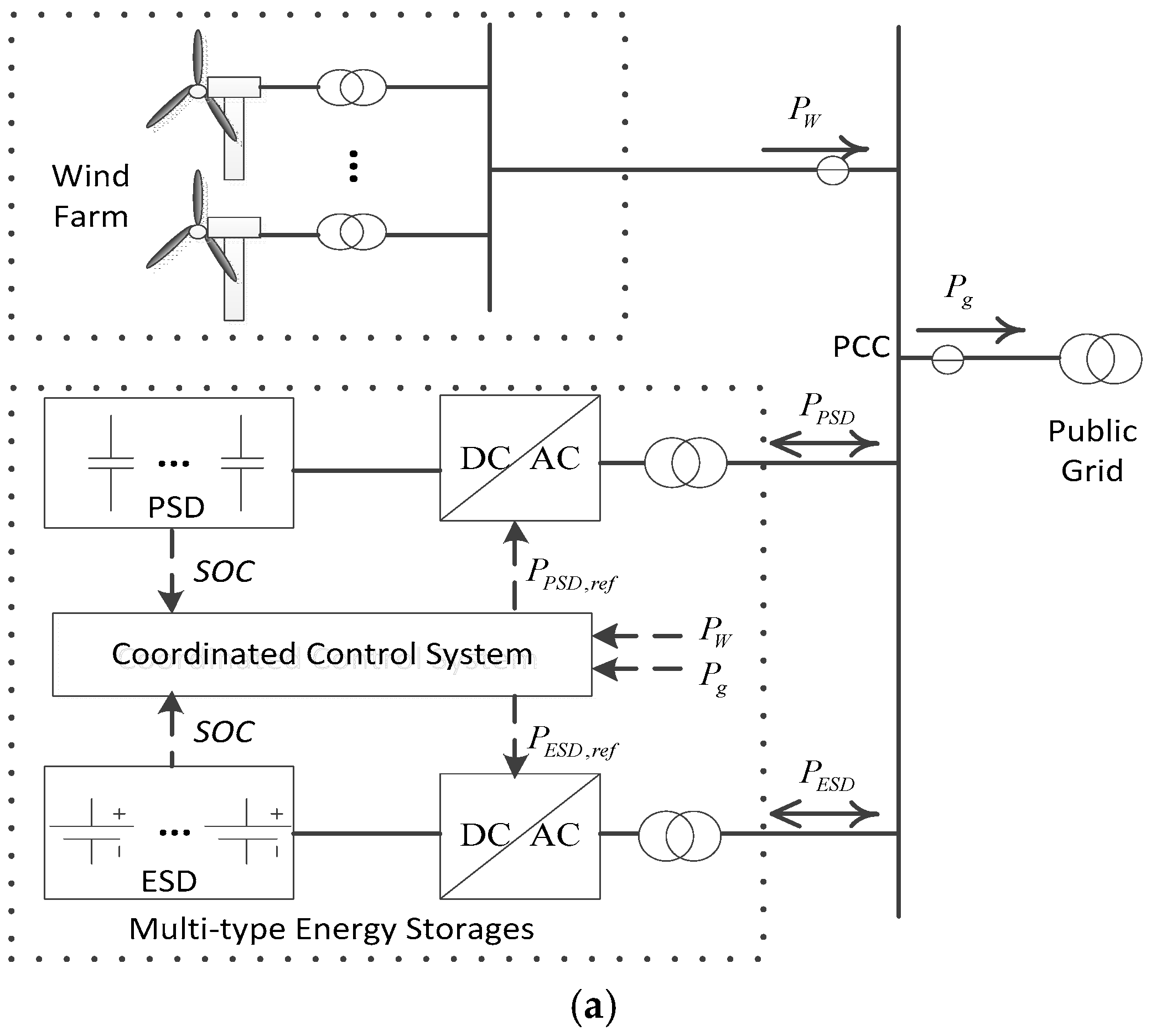
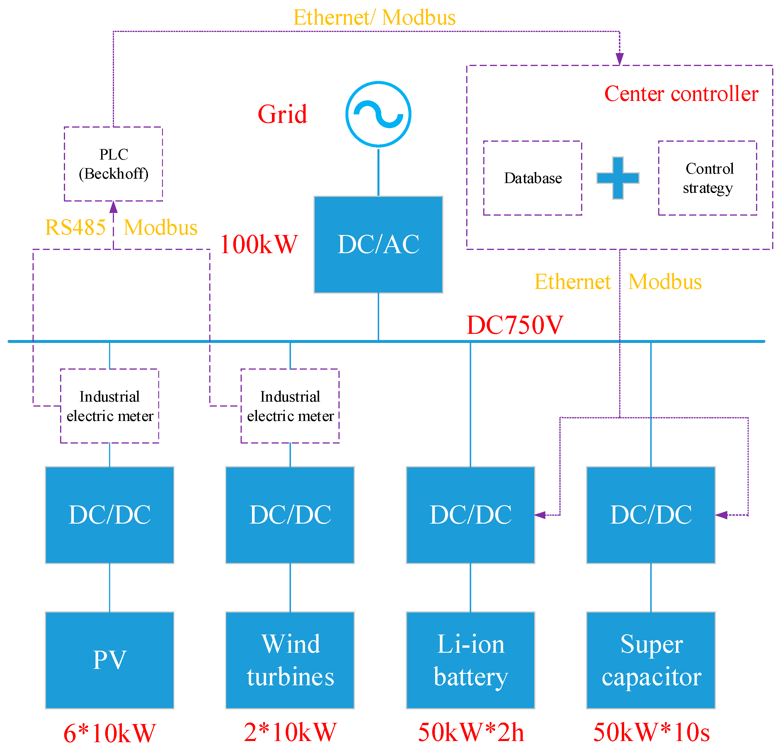
2.1. System Description

Figure 1a illustrates the structure of a multi-type energy storage system for wind farm fluctuation suppression. The ESD and PSD units are connected to the power network at the point of common coupling (PCC) together with wind farm.
Through the charging or discharging of ESD and PSD, the power fed into power system P g can be controlled within a limited value. The key issue of this system is the charging and discharging control of ESD and PSD units at each control step. As we know, an effective control strategy means less energy storage capacity required, as well longer service time and a shorter payback period [9,10].
A MPC-based control scheme is proposed in this paper, as illustrated in Figure 1b. It contains a two-level power distribution structure where the first one determines the total power requirement of the multi-type energy storage system based on the MPC algorithm. With the knowledge of wind power P w and its ramp limit calculated from P g , the load of the whole energy storage P e s can be obtained.
Then, a LFA module was used for the second-level power distribution between PSD and ESD. The basic principle was to assign the high-frequency component P P S D of wind power fluctuations to the PSD unit, and the low-frequency component P E S D to the ESD unit.
In the control system, a persistence model was used for the wind power prediction of the next few control steps. Moreover, a quadratic programming (QP) method was used in the optimizer to solve the optimization problem which will be introduced in the following section.

2.2. MPC State Space Model

The core of MPC is the receding horizon principle (RHP), which includes mainly the following steps [18]:
(i)
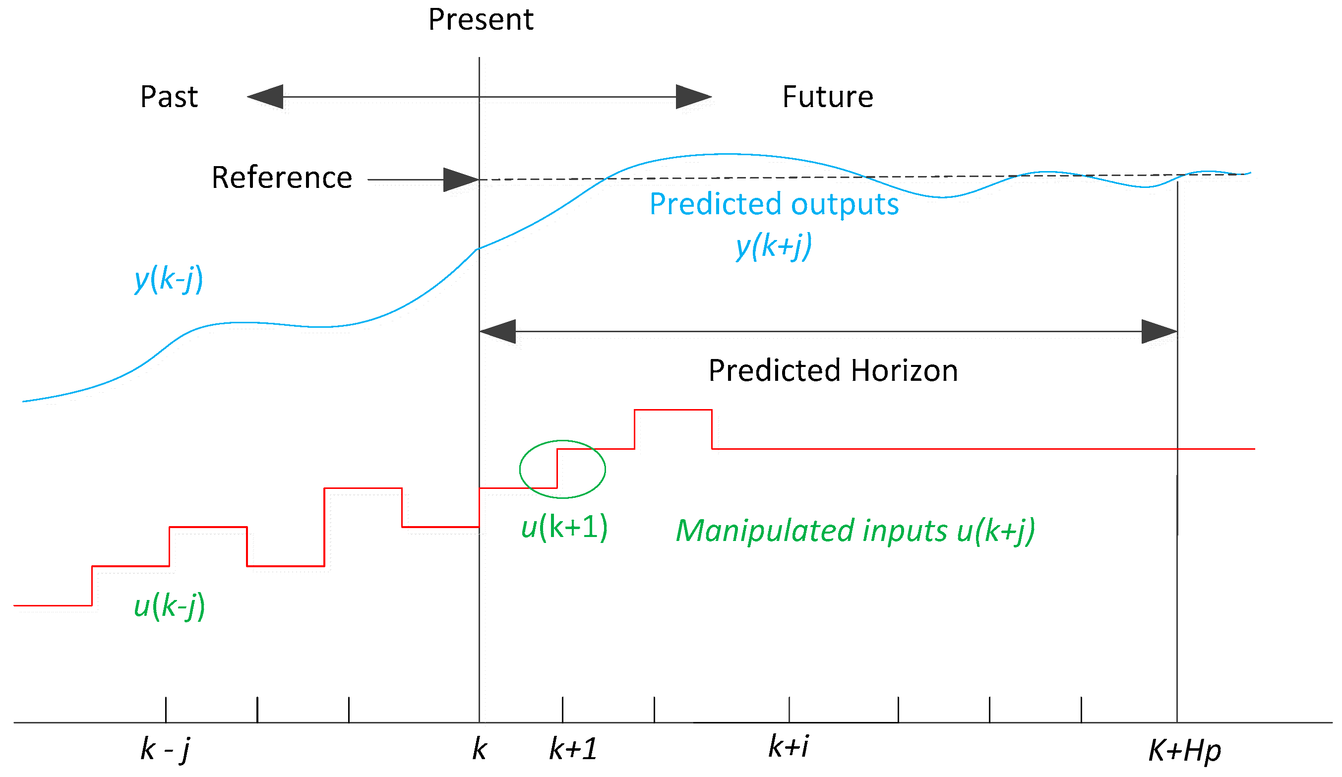
At time k and for the current state x(k), an open-loop optimal control problem is solved on-line over the next few steps taking account of the current and future constraints. Then the control instructions of the next few steps of k + 1, k + 2, …, k + Hp can be obtained, where Hp is the predicted horizon.
(ii)
Apply the instructions in the first step of k + 1 in the optimal control sequence.
(iii)
Repeat the procedure at time (k + 1) using the current state x(k + 1) as shown in Figure 2 [22], where u is the control input and y is the system output.
By the prediction of the control instructions and variations in the state of the next step and following several steps, we can make the control process more accurate and quick. As a result, the sequence u can be optimized to make the output y follow its reference better.
As an optimal control process, the state space model (SSM) is established as shown in Equations (1) and (2), assuming the current state x(k), control input u(k), disturbance input r(k), and output variable y(k).
x ( k + 1 ) = A x ( k ) + B 1 u ( k ) + B 2 r ( k )
y ( k ) = C x ( k ) + D 1 u ( k ) + D 2 r ( k )
where A, B1, B2, C, D1, and D2 are the coefficient matrices, respectively. Then the output y(k+1) of the next step can be obtained from the iteration of Equations (1) and (2)
y ( k + 1 ) = C ( A x ( k ) + B 1 u ( k ) + B 2 r ( k ) ) + D 1 u ( k + 1 ) + D 2 r ( k + 1 )
Continue the iteration until the step of the prediction horizon length of Hp, so that we can obtain the matrix equation [24].
[ y ( k ) y ( k + 1 ) y ( k + 2 ) y ( k + H p ) ] = [ C C A C A 2 C A H p ] [ x ( k ) ] + [ D 1 C B 1 0 D 1 0 0 0 0 0 0 C A B 1 C B 1 D 1 0 0 C A H p 1 B 1 C A H p 2 B 1 C A H p 3 B 1 C B 1 D 1 ] [ u ( k ) u ( k + 1 ) u ( k + 2 ) u ( k + H p ) ] + [ D 2 C B 2 0 D 2 0 0 0 0 0 0 C A B 2 C B 2 D 2 0 0 C A H p 1 B 2 C A H p 2 B 2 C A H p 3 B 2 C B 2 D 2 ] [ r ( k ) r ( k + 1 ) r ( k + 2 ) r ( k + H p ) ]
From Equation (4), it can be seen that SSM establishes the relationship among system output, current state, control input and disturbances, so that system behavior for the next several steps can be predicted. In other words, with the predictive output target and system current state known, the control instructions of the oncoming several steps can be determined from Equation (4). This can be helpful for the coordinated control of multi-type energy storage.

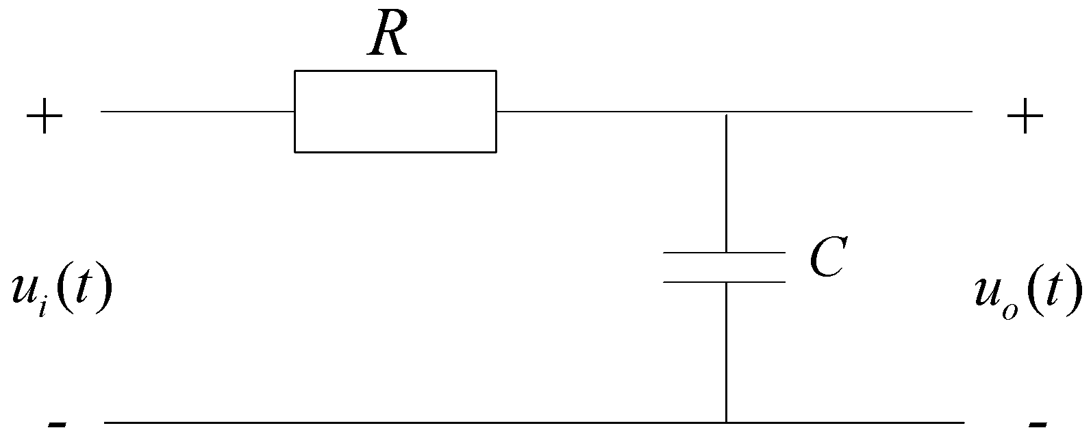
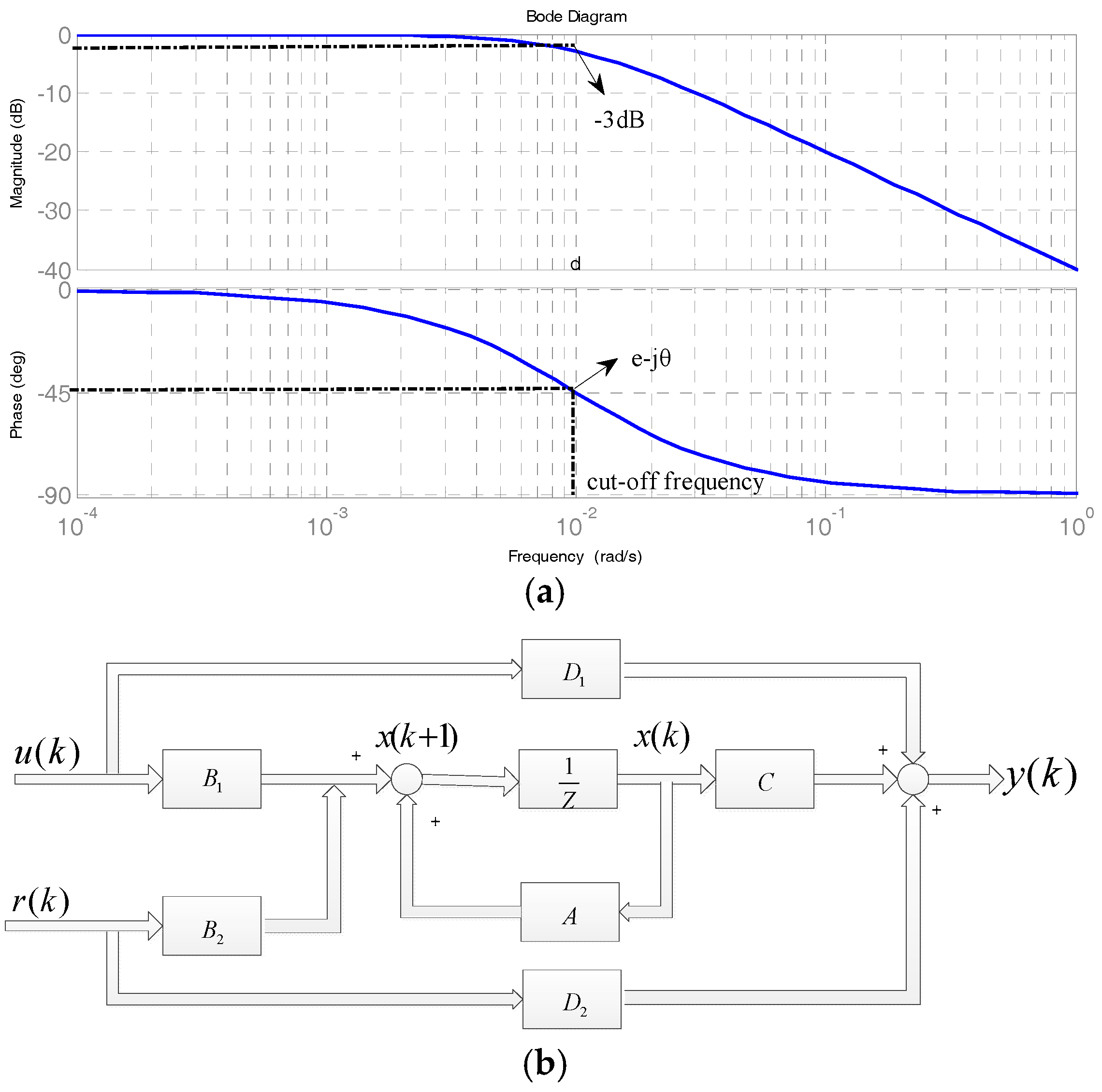
2.3. Traditional LFA

The equivalent circuit of LFA is shown in Figure 3, where R is the equivalent resistor and C the equivalent capacitor.
According to the Kirchhoff voltage law (KVL), the relationship between the input voltage and the output voltage can obtained.
R C d u o ( t ) d t + u o ( t ) = u i ( t )
Through Laplace transformation, the transfer function of output voltage to input voltage can be obtained:
H ( s ) = U o ( s ) U i ( s ) = 1 R C s + 1 = 1 τ s + 1
where τ = R C represents the LFA time constant. Through Z-transformation, it can be discretized as
H ( z ) = 1 1 + τ T c τ T c z 1 = Y ( k ) X ( k )
where T c is the control time interval; Y ( k ) the output variable; and X ( k ) the input variable.
According to Equation (7), the discretized formation of LFA output Y ( k ) as the function of input X ( k ) is
Y ( k ) = τ τ + T c Y ( k 1 ) + T c τ + T c X ( k )
In this iteration, Y ( k 1 ) = τ τ + T c Y ( k 2 ) + T c τ + T c X ( k 1 ) .
It can be seen from Equation (8) that the LFA output at time k, represented as Y(k), is associated with its output at time k – 1, represented as Y(k − 1). Moreover, it can be inferred that the larger the time constant τ , the smaller the difference between Y(k) and Y(k − 1), i.e., the smoothing effect of LFA is better. However, the time lag is bigger accordingly.
Taking the differential operator s = j ω , Equation (6) can be transformed into the complex domain
H ( j ω ) = H ( s ) | s = j ω 1 τ 2 ω 2 + 1 e j arctg ω τ
Figure 4a shows the Bode plot of Equation (9) where f c is the cut-off frequency (COF), from which LFA magnitude begins to decline quickly. The phase lag at f c , e j θ with θ = arctg ω τ , represents LFA time-lag. It can be seen that the larger the time constant τ , the greater the time delayed.
Figure 4b illustrates the control diagram of the MPC algorithm from the SSM given in Equations (1) and (2). It is clear that y(k) is independent of y(k − 1), its historic performance, and this is significantly different from LFA. This means that the current control process needs no information of the previous data and the problem of the time-lag can be avoided.
With the establishment of SSM, MPC can be solved through the increment of the control variables in the rolling time domain. At each of the control times k, the output y H p ( k + i | k ) of the next several steps can be calculated with the initial predicted value of output y 0 ( k + i | k ) and the control input increment Δ u ( k ) known, as shown in Equation (10).
y H p ( k + i | k ) = y 0 ( k + i | k ) + j = 1 min ( H p , i ) a i j + 1 × Δ u ( k + j 1 ) , i = 1 , , N
Taking R ( k + j | k ) as the expected output at time k + j, the objective of MPC is to minimize the absolute error between the future output y ( k + j | k ) and the expected output R ( k + j | k ) , as shown in Equation (11).
J = min j = 1 H p [ R ( k + j | k ) y H p ( k + j | k ) ] 2 = min j = 1 H p [ R ( k + j | k ) y 0 ( k + j | k ) j = 1 min ( H p , i ) a i j + 1 × Δ u ( k + j 1 ) ] 2 , i = 1 , , N
Therefore, MPC is implemented through the adjustment of the control input increment Δ u ( k ) to eliminate the error between the expected output R ( k + j | k ) and the predicted output y ( k + j | k ) . Compared with traditional PID (Proportion Integration Differentiation) control, MPC has better predictability to compensate the error between the expected output R ( k ) and the current output y ( k ) [25].

3. Coordinated Control Scheme

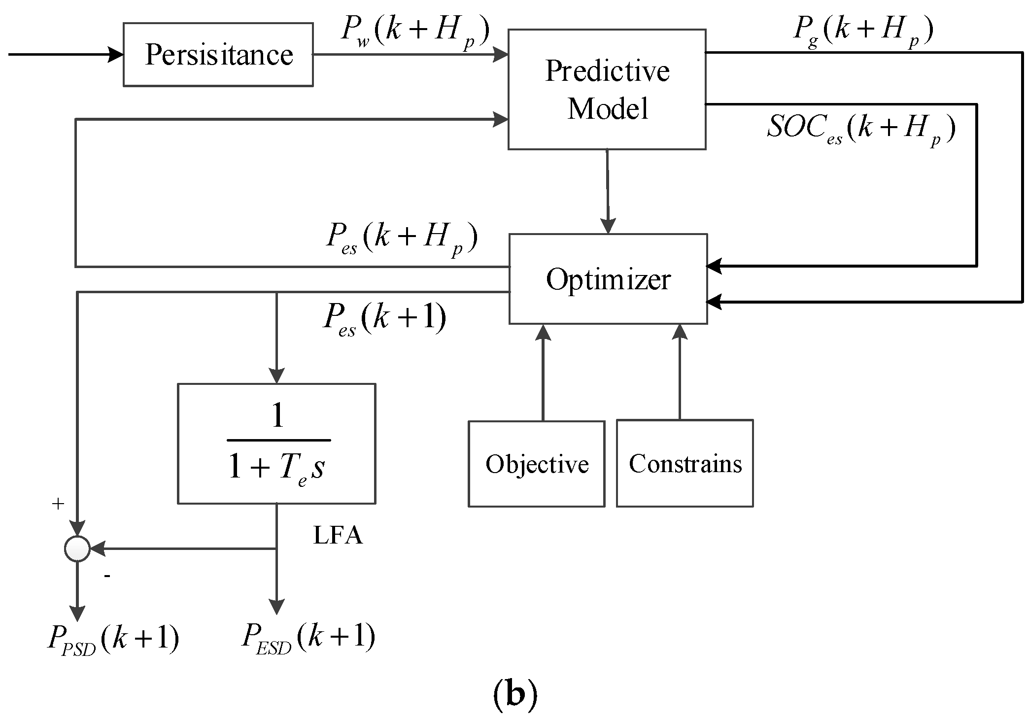
3.1. MPC Control for Energy Storage Systems

From Figure 1, the relations of the variables in the wind/storage system can be expressed according to the following equations
P g ( k + 1 ) = P e s ( k ) + P w ( k )
S O C ( k + 1 ) = S O C ( k ) T c · P e s ( k ) / C e s
where P g is the power output to the grid; P w the wind power output; P e s the power output of the total energy storage system; S O C ( k ) the equivalent state of charge (SOC) of the energy storage system at time k; T c the control time interval; and C e s the capacity of energy storage.
Taking P g and S O C as state variables x 1 and x 2 respectively; P e s as the control variable u ; and P w as disturbance input r , Equations (12) and (13) can be written in the state space model (SSM)
[ x 1 ( k + 1 ) x 2 ( k + 1 ) ] = [ 0 0 0 1 ] [ x 1 ( k ) x 2 ( k ) ] + [ 1 T c ] [ u ( k ) ] + [ 1 0 ] [ r ( k ) ] [ y 1 ( k ) y 2 ( k ) ] = [ 1 0 0 1 ] [ x 1 ( k ) x 2 ( k ) ]
Continue the iterations until step H p , and then a matrix similar to Equation (4) can be obtained. Meanwhile, the control sequence of u ( k ) , u ( k + 1 ) , , u ( k + H p ) at each control step can be obtained through the MATLAB QP Toolbox [18,24].
Then the control variables of the SSM can be standardized in the following formation
U O P T = [ u O P T ( k ) , u O P T ( k + 1 ) , , u O P T ( k + H p ) ] T
The above control variables can be obtained through numerical calculation, i.e., they can be converted into the solving of the following static optimization problem
U O P T = arg min U T W U + 2 U T V U L U K
where W is the coefficient matrix of the quadratic term of U 2 , and V the coefficient matrix of U .
As to wind power fluctuation suppression, the wind farm output power rate to the public utility is considered as a basic constraint to be satisfied. The target of the coordinated control of the energy storage system is to reduce the usage of energy storage, which means the reduction of power losses and prolonging the life of energy storage. Therefore, the optimization problem can be equivalent to a model with the objective of minimizing energy storage usage, and limiting the constraints of wind power fluctuation rates, SOC and the charging/discharging power limit of energy storage, as shown in Equations (17)–(21).
Objective:
J = min i = k k + H p P e s 2 ( i )
Constraints:
0 P g ( k ) P g _ max ; k = 1 , 2 , , H p
0 S O C es ( k ) 1 ; k = 1 , 2 , , H p
P es _ min P e s ( k ) P e s _ max ; k = 1 , 2 , , H p
max i = 1 , 2 , n P g ( k i ) min i = 1 , 2 , n P g ( k i ) P wind _ r a t e d γ ;     k = 1 , 2 , , H p
where Equation (17) is the objective of minimizing energy storage usage. The charging/discharging power of energy storage is defined as negative/positive in this paper, so the sum of the squares of power is used as the optimization target. Equation (18) is the power constraint of wind farms injected into the grid, Equation (19) the SOC constraint of energy storage, Equation (20) the charging/discharging power limit of energy storage, Equation (21) the fluctuation rate limit of wind farms, with P wind _ r a t e d its rated power.

3.2. Power Allocation between PSD and ESD

As shown in Figure 2, LFA is adopted for the power allocation between PSD and ESD units. The total power demand is filtered by LFA and the output, which is the low frequency part of the total power demand, is assigned as the power reference of ESD; while the remains, which is the high frequency part, is assigned as the power reference of PSD.
As to LFA, its COF f c can be written as
f c = 1 / 2 π τ
Obviously, f c is inversely proportional to the time constant τ . The larger the τ , the smaller the COF f c , i.e., more fluctuating power should be compensated by PSD, while that of ESD is reduced, and vice versa. Practically, the COF f c can be altered in the control process according to energy storage configuration and SOC. It will be discussed in Section 5.
Although there is some time delay in the second power allocation stage due to the use of LFA, the fluctuation suppression effect would not be affected since the total power required can be satisfied with the fast response of PSD.

3.3. Simulation Flowchart

(1)
Wind power data is imported from database;
(2)
Persistence model is established to get wind power at time k + Hp based on wind power at time k;
(3)
If the wind power data length is greater than Hp, SSM can be established; Otherwise, go back to step 1;
(4)
Constraint matrix is established on the basis of the fluctuation rate;
(5)
The total energy storage power is obtained by using the QP Toolbox to solve the quadratic programming equation;
(6)
P P S D (PSD power) and P E S D (ESD power) are allocated with LFA.

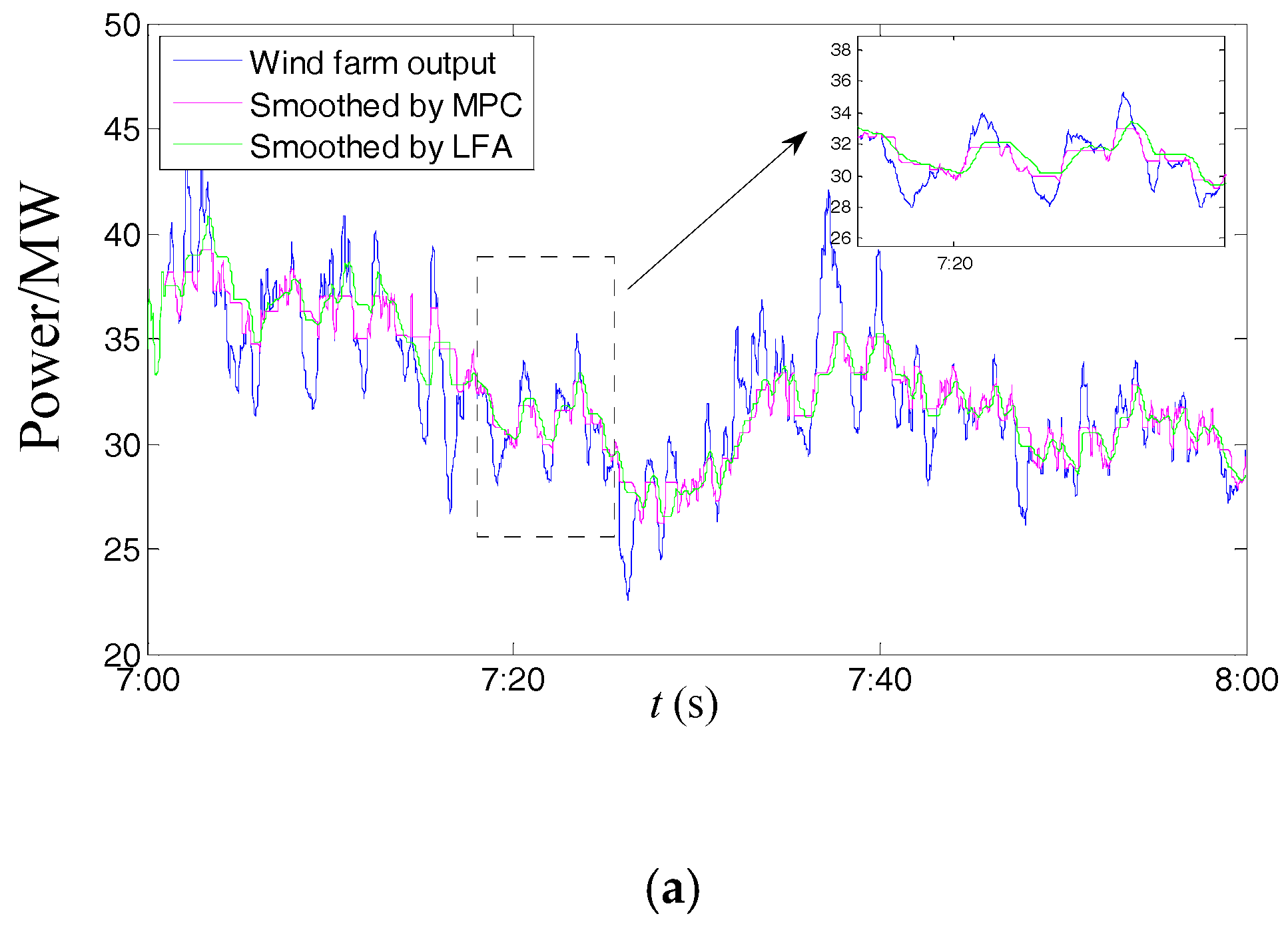
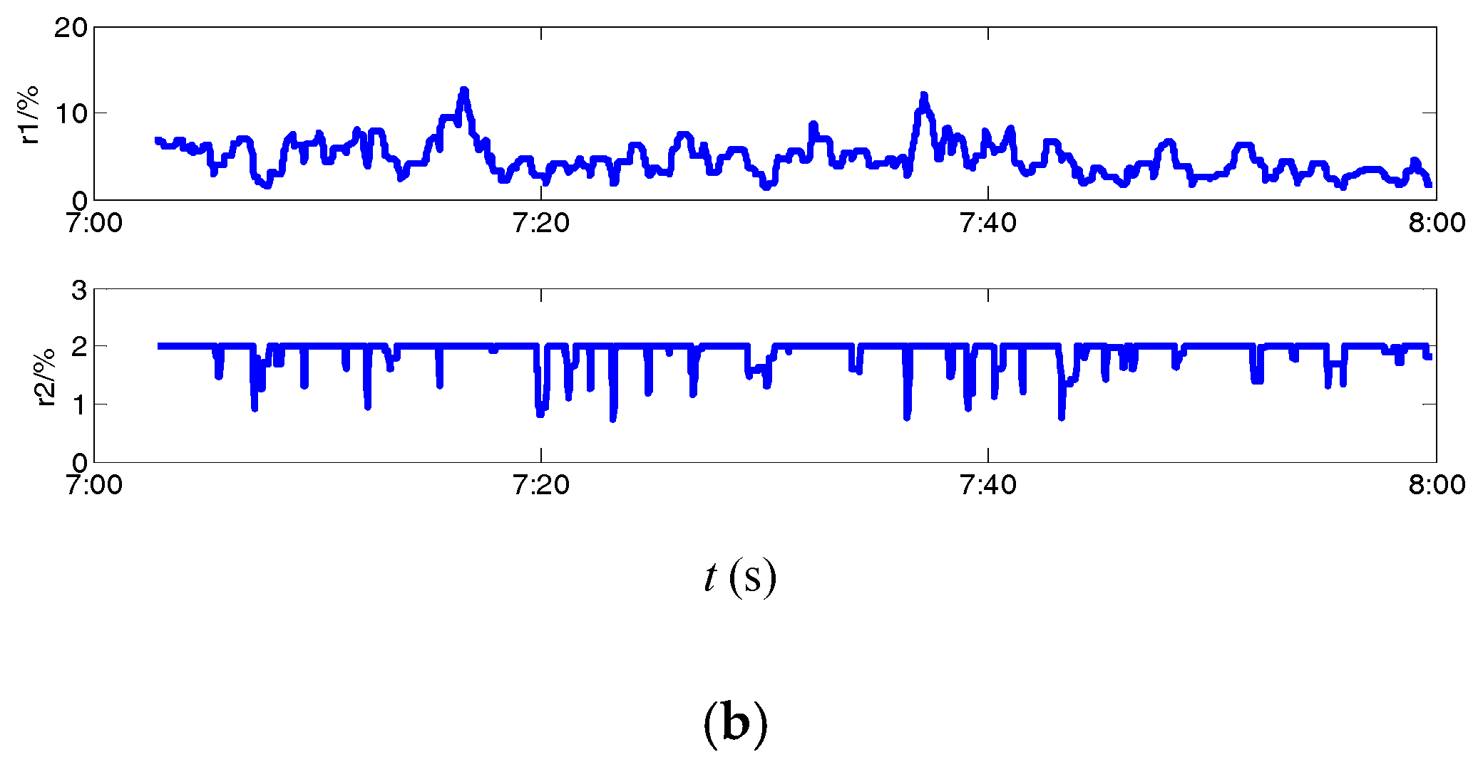
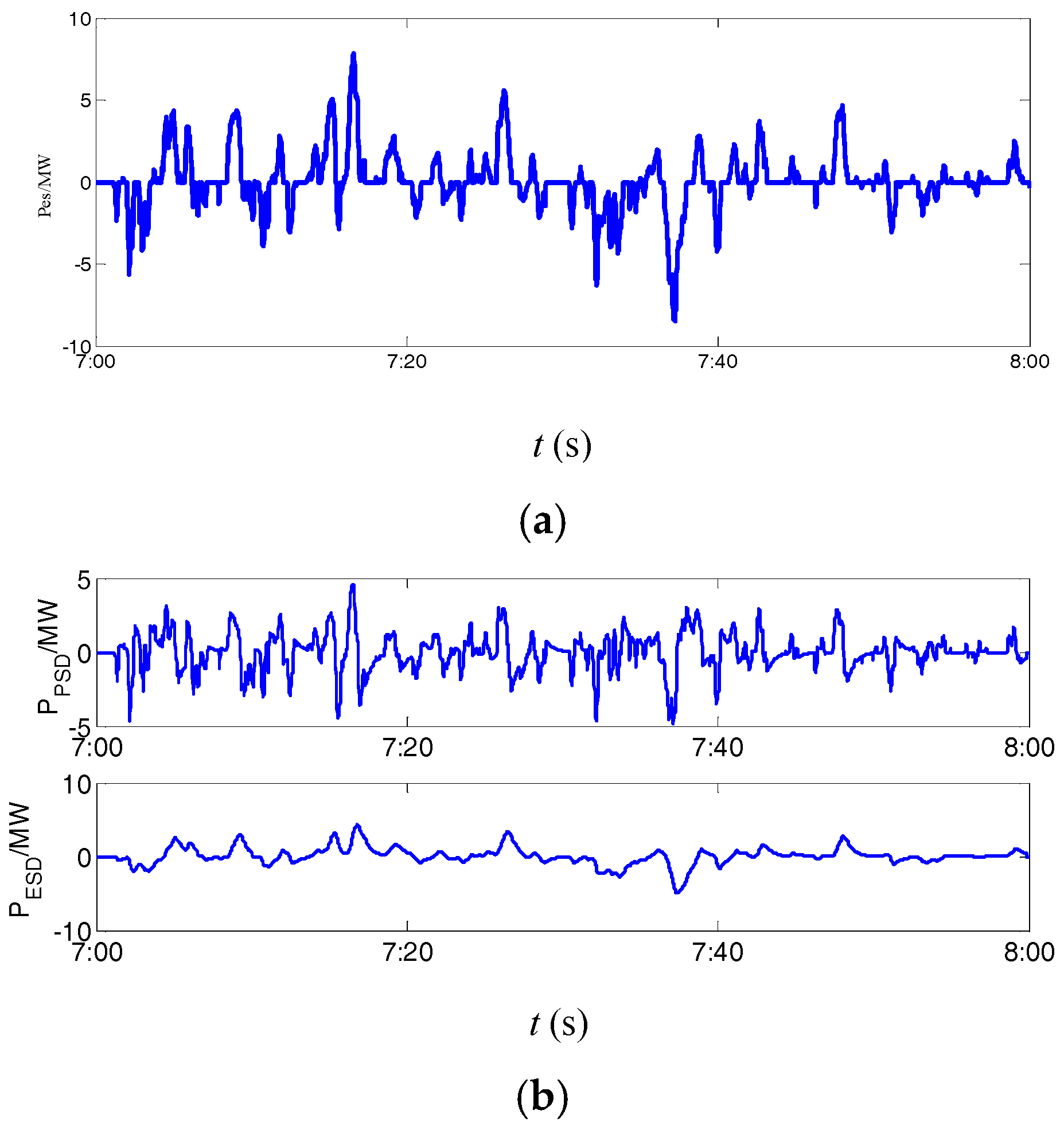
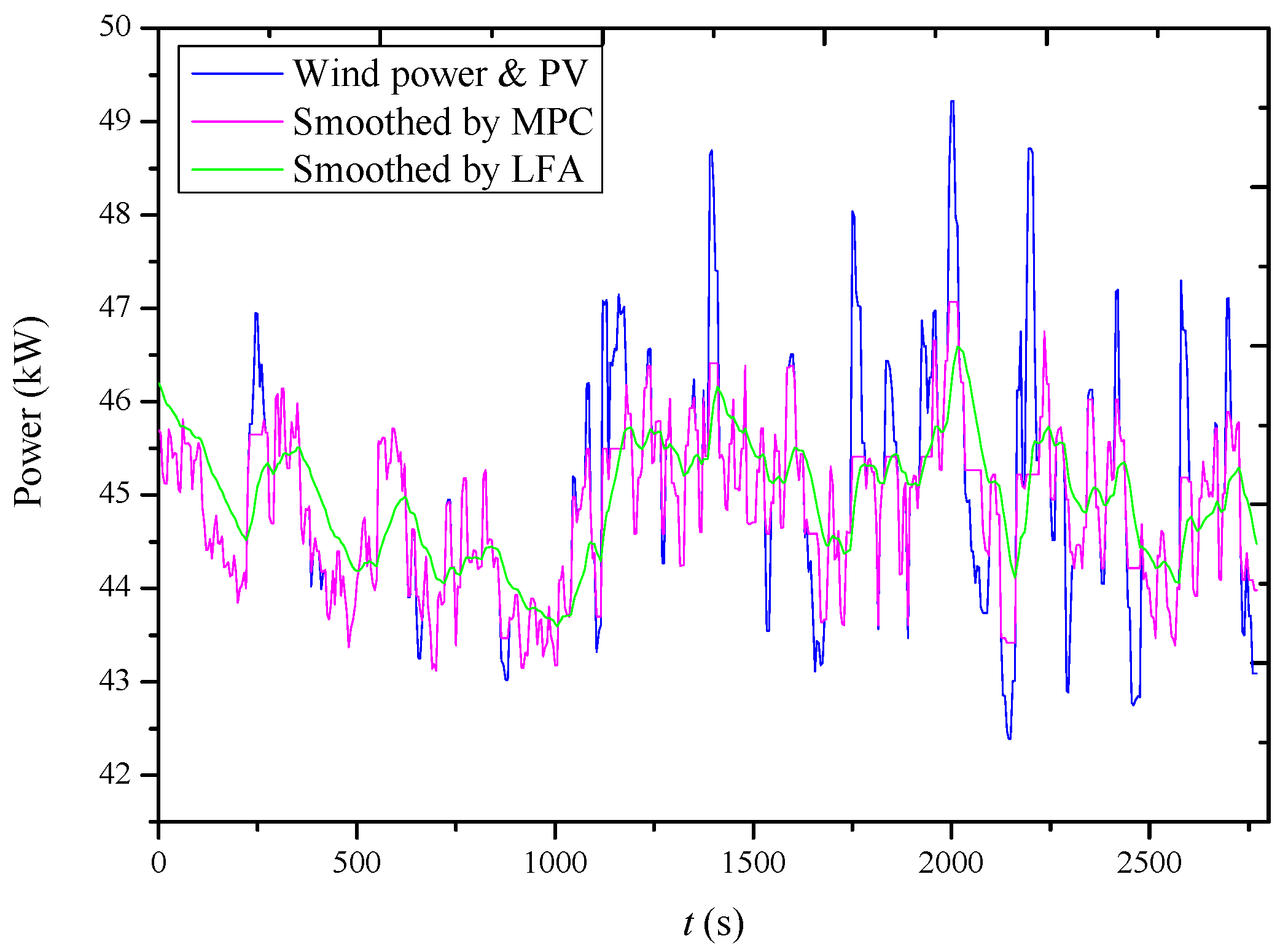
4. Simulation and Experiment Results

In order to verify the proposed control strategies, a simulation platform based on Matlab/Simulink was set up with a 100 MW wind farm, 20 MW Li-ion batteries and 20 MW SC energy storage systems.
The actual data of the wind farm output power of a typical period was imported into the simulation system one by one with a time interval of 1 s to simulate the actual wind power output. According to the grid codes in China and some other countries, the power fluctuation of the wind farm in this paper is limited within 2% of its rated power per minute [4], since wind power fluctuation in this time scale may influence the frequency control of the power system.
According to the flowchart shown in Figure 5, the simulation results based on the proposed MPC method were able to be achieved, which will be compared with LFA.
It can be seen from Figure 6a that the wind farm output power fluctuation ratio of P g can be suppressed with both MPC and LFA control methods. The fluctuation ratio per minute can be limited within 2%, as shown in Figure 6b. The detailed curve in Figure 6a can also illustrate that the MPC based method has much less time delay than that of LFA since the integrated power with MPC follows the original wind power more tightly. This verifies the control timeliness of MPC, which takes into account future constraints at the current control step and carries out optimal control in advance.
The total energy storage power needed of P e s is given in Figure 7a with MPC control. Through LFA, P P S D (PSD power) and P E S D (ESD power) are allocated automatically, as shown in Figure 7b. It can be seen that PSD suppresses the high-frequency power fluctuations, while ESD suppress the low-frequency ones. This fits the complementary features of PSD and ESD.
As to the power and energy capacity required for the energy storage system, a comparison between MPC and LFA is given in Table 2. It can be seen that 4.1% power and 23.5% energy can be saved through the MPC based method for the 100 MW wind farm in the simulation.
Additionally, a microgrid demonstration system was utilized to verify the proposed algorithm. The microgrid demonstration system was a DC microgrid, whose bus voltage is 750 V. It connected to the power grid through the DC/AC converter. It had 20 kW wind power, 60 kWp PV, a 50 kW Li-ion battery energy storage system and a 50 kW SC energy storage system. As can be seen from Figure 8, the information on wind power and PV, including current, power and so on, was read by the industrial electric meters. Then the information was uploaded to the PLC (Beckhoff product) through RS485/Modbus. The center controller received the information on wind power and PV from the PLC and issued the control instructions calculated by the control strategy to the multi-type energy storage system through Ethernet/Modbus. Firstly, MPC was adopted in the center controller to smooth the total fluctuation of wind power and PV. Then the actual data was stored in the database and analyzed again off-line with LFA method. As shown in Figure 9, the MPC-based method can be more effective compared with LFA in a condition of less time delay. In particular, about 5% power and 15% energy can be saved, as shown in Table 3.

5. Discussion

The impacts of different wind speed levels and the LFA cut-off frequency on multi-type energy storage sizes are further discussed with the simulation platform based on Matlab/Simulink presented at the beginning of Section 4.

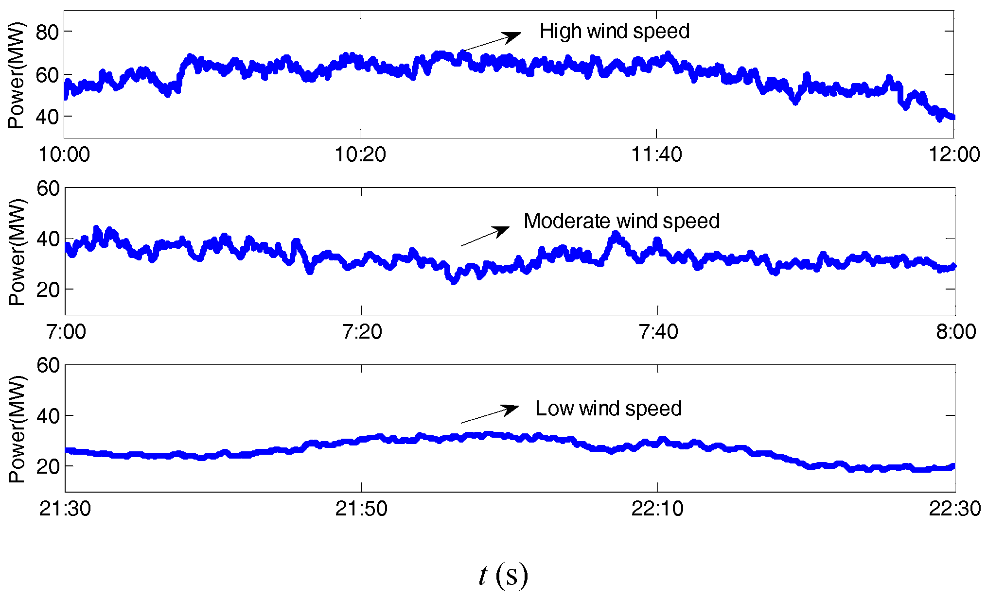
5.1. Different Wind Speed Level

Wind speed conditions influenced the wind/storage control process since wind power varies obviously with wind speed, and so do the fluctuations. Given different data samples in the simulations, the results were greatly different, as shown in Table 4. The installed capacity and sampling interval of wind power was 100 MW and 1 s in the data samples, which is the same as Figure 6a. However, the total power and energy saving was able to be achieved for MPC.
The active power output of a wind turbine is
P w = 1 2 ρ π R 2 C p ( λ , β ) v w 3
where ρ is the air density; β the blade pitch angle; R the wind turbine radius; and v w the wind speed. λ is the ratio of blade tip speed to wind speed given by λ = ω R / v w with ω wind turbine rotational speed. The power coefficient C p is the function of λ and β .
With all the parameters of the wind turbine determined, the derivation of wind power to wind speed v w can be written as:
d P w d v w = 3 2 ρ π R 2 C p ( λ , β ) v w 2
It can be seen that, for a certain wind turbine and certain wind speed changes, the power variation is proportional to the square of the initial wind speed. This means that a small wind speed variation may cause a large wind power fluctuation, especially at high wind speed. Although there are smooth effects for a wind farm with clusters of wind turbines, the fluctuations of output power are still high with wind speed variations. Figure 10 shows the wind power and the corresponding fluctuating levels at high, moderate and low wind speeds, respectively.
A simulation system is set up to verify the differences between multi-type energy storage systems required under various wind speed conditions as shown in Table 5. According to the response time of Li-ion batteries (used as ESD) and SC (used as PSD), several LFA time constants are chosen from 1 s to 160 s. It can be seen that the maximum fluctuation per minute under high wind speeds is 16.35%. In this case, a large amount of power and energy for energy storage was required to suppress wind power fluctuations, with a SC of 9.8208 MW/0.3155 MWh and a Li-ion battery of 3.8737 MW/0.6347 MWh, respectively, with COF of 0.001 Hz. The values decrease to 7.0857 MW/0.1676 MWh and 1.9984 MW/0.2237 MWh under moderate wind speeds and decrease again to 1.3895 MW/0.0151 MWh and 0.1949 MW/0.0167 MWh under low wind speeds with the same COF.
Therefore, the power and energy requirements of energy storage may differ greatly with the variation of wind conditions. In other words, if the wind speed conditions of the oncoming time are known, the SOC of the energy storages can be controlled in advance to a certain level to be ready for the charging/discharging energy needed. In this way, ultra-short term or real-time wind condition forecasting can be helpful for wind/storage coordinated control.

5.2. Different LFA Cut-off Frequency

LFA was adopted in this paper for the power and energy allocation between PSD and ESD, and the COF was found to be a key factor which directly determines the usage of PSD and ESD according to Equation (6). From Table 5, it can be seen that under certain wind conditions, the amount of PSD power and energy covered decreased gradually as COF increased, while ESD increased accordingly. In the case of high wind speeds, with COF increasing from 0.001 Hz to 0.1 Hz, the power demand of SC falls from 9.82 MW to 3.61 MW and the corresponding energy demand falls from 0.32 MWh to 0.01 MWh, while that of the Li-ion battery increases at the same time.
Therefore, LFA COF can be changed flexibly in wind/storage control according to wind power output and the SOC of each of the energy storage units. For example, when PSD SOC is low in some periods, LFA COF can be made smaller to discharge more ESD, and vice versa. A proper LFA time constant can make the operation of both PSD and ESD units fit their technical specifications and configure their capacity. As a result, the technical economy effect of the whole energy storage system can be enhanced.

6. Conclusions

With the rapid development of wind power, its stochastic fluctuations may impose special requirements on power system operation, such as spinning reserve and power dispatching. Energy storage, especially the combination of PSD and ESD, have the feasibility both technically and economically for wind power fluctuation suppression.
In this paper, a multi-type energy storage system containing both PSD and ESD was presented for wind farm power fluctuation suppression with the high-frequency fluctuations compensated by PSD and the low-frequency fluctuations compensated by ESD. The contribution of this paper is the combination of MPC and LFA for the coordinated control of PSD and ESD. The MPC-based method was used to determine the total power required of the whole energy storage system, and then LFA was used to allocate the power between ESD and PSD. Due to the predictive feature of MPC, wind power fluctuations can be limited with less energy storage used compared with traditional LFA-based method. Moreover, the influences of wind speed conditions and LFA COF for ESD and PSD allocation are obvious for the power and energy needed. Multiple time scale wind power fluctuations can be mitigated effectively by multi-type energy storage with the proposed control strategy. Energy storage size will be reduced and its cycle life will be improved. To consider them practically can be helpful for better control performance for the wind/storage system control. This can promote the large-scale development of renewable energy and the industrial application of multi-type energy storage.

Acknowledgments

This work was financially supported by a grant from the National Key Research and Development Program of China (No. 2016YFB0900400), Foundation of Director of Institute of Electrical Engineering, Chinese Academy of Sciences (No. Y760141CSA) and Jiangsu Province 2016 Innovation Ability Construction Special Funds (BM2016027).

Author Contributions

Xisheng Tang and Yushu Sun designed the main parts of the study, including control design, and the implementation of simulation and experiment. Guopeng Zhou and Fufeng Miao mainly worked on the simulation and the writing of paper.

Conflicts of Interest

The authors declare no conflict of interest.

References

  1. Lotfi, B.; Najiba, B.M.; el Euch, M. Impact of wind power integration on operating reserves. In Proceedings of the 16th IEEE Electrotechnical Conference (MELECON), Yasmine Hammamet, Tunisia, 25–28 March 2012; pp. 67–71. [Google Scholar]
  2. Guo, H.; Rudion, K.; Styczynski, Z.A. Integration of large offshore wind farms into the power system. In Proceedings of the 2011 EPU-CRIS International Conference on Science and Technology, Hanoi, Vietnam, 16 November 2011; pp. 1–6. [Google Scholar]
  3. Chávez, H.; Baldick, R.; Sharma, S. Governor rate-constrained OPF for primary frequency control adequacy. IEEE Trans. Power Syst. 2014, 29, 1473–1480. [Google Scholar] [CrossRef]
  4. Jiang, Q.; Hong, H. Wavelet-based capacity configuration and coordinated control of hybrid energy storage system for smoothing out wind power fluctuations. IEEE Trans. Power Syst. 2013, 28, 1363–1372. [Google Scholar] [CrossRef]
  5. Lee, H.; Shin, B.Y.; Han, S.; Jung, S.; Park, B.; Jang, G. Compensation for the power fluctuation of the large scale wind farm using hybrid energy storage applications. IEEE Trans. Appl. Supercond. 2011, 22. [Google Scholar] [CrossRef]
  6. Li, X.; Hui, D.; Lai, X. Battery energy storage station (BESS)-based smoothing control of Photovoltaic (PV) and wind power generation fluctuations. IEEE Trans. Sustain. Energy 2013, 4, 464–473. [Google Scholar] [CrossRef]
  7. Miao, F.; Tang, X.; Qi, Z. Fluctuation feature extraction of wind power. In Proceedings of the PES Innovative Smart Grid Technologies (ISGT), Tianjin, China, 21–24 May 2012; pp. 1–5. [Google Scholar]
  8. Barton, J.P.; Infield, D.G. Energy storage and its use with intermittent renewable energy. IEEE Trans. Energy Convers. 2004, 19, 441–448. [Google Scholar] [CrossRef]
  9. Li, W.; Joós, G.; Bélanger, J. Real-time simulation of a wind turbine generator coupled with a battery supercapacitor energy storage system. IEEE Trans. Ind. Electron. 2010, 57, 1137–1145. [Google Scholar] [CrossRef]
  10. Gee, A.M.; Dunn, R.W. Novel battery supercapacitor hybrid energy storage control strategy for battery life extension in isolated wind energy conversion systems. In Proceedings of the 45th International Universities Power Engineering Conference (UPEC), Wales, UK, 31 August–3 September 2010; pp. 1–6. [Google Scholar]
  11. Gonzalez, F.D.; Bianchi, F.D.; Sumper, A. Control of a flywheel energy storage system for power smoothing in wind power plants. IEEE Trans. Energy Convers. 2014, 29, 204–214. [Google Scholar]
  12. Wu, G.; Yoshida, Y.; Minakawa, T. Mitigation of wind power fluctuation by combined use of energy storages with different response characteristics. Energy Procedia 2011, 12, 975–985. [Google Scholar] [CrossRef]
  13. Tankari, M.A.; Camara, M.B.; Dakyo, B.; Nichita, C. Attenuation of power fluctuations in wind diesel hybrid system—Using ultracapacitors and batteries. In Proceedings of the XIX International Conference on Electrical Machines—ICEM 2010, Incheon, Korea, 25 October 2010; pp. 1–6. [Google Scholar]
  14. Jia, H.; Fu, Y.; Zhang, Y.; He, W. Design of hybrid energy storage control system for wind farms based on flow battery and electric double-layer capacitor. In Proceedings of the APPEEC, Chengdu, China, 28–31 March 2010; pp. 1–6. [Google Scholar]
  15. Ding, M.; Lin, G.; Chen, Z. A control strategy for hybrid energy storage systems. Proc. CSEE 2012, 32, 1–7. [Google Scholar]
  16. Zhang, G.; Tang, X.; Qi, Z. Design of a hybrid energy storage system on leveling off fluctuation power outputs of intermittent sources. Autom. Electron. Power Syst. 2011, 35, 24–28. [Google Scholar]
  17. Senjyu, T.; Kikunaga, Y.; Yona, A.; Sekine, H.; Saber, A.Y.; Funabashi, T. Coordinate control of wind turbine and battery in wind power generator system. In Proceedings of the 2008 IEEE Power and Energy Society General Meeting—Conversion and Delivery of Electrical Energy in the 21st Century, Detroit, MI, USA, 24–28 July 2011; pp. 1–7. [Google Scholar]
  18. Goodwin, G.C.; Graebe, S.F.; Salgado, M.E. Control System Design; Valparaıso, P., Ed.; McGraw-Hill: New York, NY, USA, 2000. [Google Scholar]
  19. Mayhorn, E.; Kalsi, K.; Lian, J.; Elizondo, M. Model predictive control-based optimal coordination of distributed energy resources. In Proceedings of the 2013 46th Hawaii International Conference on System Sciences, Maui, HI, USA, 7–10 January 2013; pp. 2237–2244. [Google Scholar]
  20. Borhan, H.A.; Vahidi, A. Model predictive control of a power-split Hybrid Electric Vehicle with combined battery and ultracapacitor energy storage. In Proceedings of the 2010 American Control Conference, Baltimore, MD, USA, 30 June–2 July 2010; pp. 5031–5036. [Google Scholar]
  21. Galus, M.D.; La, F.R.; Andersson, G. Investigating PHEV wind balancing capabilities using heuristics and model predictive control. In Proceedings of the IEEE Power and Energy Society General Meeting, Minneapolis, MN, USA, 25–29 July 2010; pp. 1–8. [Google Scholar]
  22. MPC Lab. Courses of Model Predictive Control Lab @ UC-Berkeley. Available online: http://www.mpc.berkeley.edu/mpc-course-material (accessed on 3 November 2013).
  23. Maciejowski, J.M. Predictive Control with Constraints; Pearson Education: Harlow, UK, 2001. [Google Scholar]
  24. Shen, Y. Design approaches research and application of control system with input and output constraints. Ph.D. Thesis, Shandong University, Jinan, China, May 2009. [Google Scholar]
  25. Wang, L. Model Predictive Control System Design and Implementation Using MATLAB; Springer-Verlag: London, UK, 2009. [Google Scholar]
Figure 1. (a) Multi-type energy storage for wind power fluctuation smoothing; (b) Coordinated control based on MPC. (Hp is MPC predicted horizon).
Energies 10 01212 g001aEnergies 10 01212 g001b
Figure 2. Receding horizon principle of MPC [23].
Energies 10 01212 g002
Figure 3. Equivalent circuit of LFA.
Energies 10 01212 g003
Figure 4. (a) Bode plot of LFA ( τ = 100 ); and (b) structure diagram of MPC SSM.
Energies 10 01212 g004
Figure 5. Flowchart of the MPC-based coordinated control algorithm.
Energies 10 01212 g005
Figure 6. (a) Wind farm output power smoothed by MPC and LFA respectively; (b) Power fluctuation ratio without ( γ 1 ) and with ( γ 2 ) smooth control
Energies 10 01212 g006aEnergies 10 01212 g006b
Figure 7. (a) Power profile P e s of the total energy storage system; (b) Power profile of PSD ( P P S D ) and ESD ( P E S D ).
Energies 10 01212 g007
Figure 8. Microgrid system structure.
Energies 10 01212 g008
Figure 9. Experiment result of fluctuation suppression for the microgrid.
Energies 10 01212 g009
Figure 10. Comparison of wind power at different wind speeds.
Energies 10 01212 g010
Table 1. The advantages and disadvantages of the algorithms.
AlgorithmsAdvantagesDisadvantages
LFA with fixed time constantSimple, reliable, easy to engineeringtime constant cannot be adjusted; easy to cause wind power to be overly mitigated, increase energy storage cost; control delay
LFA with variable time constantSimple, reliable, easy to engineeringcontrol delay, not good for on-line control
Waveleteasy to implement frequency decompositionits difficulty lies in the selection of wavelet functions and a large amount of historical data on wind power needed
MPCgood forecast ability, control time delay can be omitted, suitable for online optimizing control-
Table 2. Power and energy requirements *.
Control MethodLFAMPCSaved (%)
Power (MW)8.82348.46354.1
Energy (MWh)0.35450.271323.5
* The power and energy required can be calculated: P e s _ r a t e d = max | P e s | E e s _ r a t e d = max E e s ( k ) min E e s ( k ) E e s ( k ) = E e s ( k 1 ) P e s ( k ) · T c / 3600 .
Table 3. Power and energy requirements.
Control MethodLFAMPCSaved (%)
Power (MW)3.67333.49004.99%
Energy (MWh)0.06790.057715.02%
Table 4. Comparison of power and energy requirements for different samples.
Control MethodLFAMPCSaved (%)
Data 1Power (MW)7.30196.476611.30
Energy (MWh)0.41860.170259.34
Data 2Power (MW)11.23799.379216.54
Energy (MWh)5.33353.624832.04
Data 3Power (MW)8.15644.781641.38
Energy (MWh)2.04280.992451.42
Data 4Power (MW)14.325112.543412.44
Energy (MWh)2.30511.364140.82
Data 5Power (MW)18.015917.24624.27
Energy (MWh)3.71063.48955.95
Table 5. Energy storage power and energy requirement with different wind speed conditions and COF. γ 1 : Fluctuation ratio of wind power; γ 2 : Fluctuation ratio limit; P s c , max : Maximum power of supercapacitor; P L B , max : Maximum power of Li-ion Battery; E s c , max : Maximum energy of supercapacitor; E L B , max : Maximum energy of Li-ion Battery.
Wind Speed γ 1 , max
(%)
γ 2 , max
(%)
fc (Hz) τ ( s ) PSC,max
(MW)
ESC,max
(MWh)
PLB,max
(MW)
ELB,max
(MWh)
High16.3520.001159.249.82080.31553.87370.6347
16.3520.0115.926.1270.07519.20460.587
16.3520.053.184.5540.017910.72290.6122
16.3520.11.593.6070.009211.03190.6153
Moderate12.7220.001159.247.08570.16761.99840.2237
12.7220.0115.924.17270.05296.57140.2681
12.7220.053.182.15460.01398.25120.2712
12.7220.11.591.32930.00718.39640.2713
Low3.4120.001159.241.38950.01510.19490.0167
3.4120.0115.921.07720.0060.77920.0192
3.4120.053.180.60821.80 × 10−31.20090.0192
3.4120.11.590.41789.80 × 10−41.2680.0192

