Abstract
The fast-growing wind power industry faces the challenge of reducing operation and maintenance (O&M) costs for wind power plants. Predictive maintenance is essential to improve wind turbine reliability and prolong operation time, thereby reducing the O&M cost for wind power plants. This study presents a solution for predictive maintenance of wind turbine generators. The proposed solution can: (1) predict the remaining useful life (RUL) of wind turbine generators before a fault occurs and (2) diagnose the state of the wind turbine generator when the fault occurs. Moreover, the proposed solution implies low-deployment costs because it relies solely on the information collected from the widely available supervisory control and data acquisition (SCADA) system. Extra sensing hardware is needless. The proposed solution has been deployed and evaluated in two real-world wind power plants located in China. The experimental study demonstrates that the RUL of the generators can be predicted 18 days ahead with about an 80% prediction accuracy. When faults occur, the specific type of generator fault can be diagnosed with an accuracy of 94%.
1. Introduction
With the ever-increasing installation capacity of wind power [1], how to reduce the operation and maintenance (O&M) costs has become a growing challenge for wind farms. O&M costs account for approximately 10–15% and 20–25% of the overall energy generation cost for onshore and offshore wind power plants, respectively [2]. In particular, wind turbine downtime significantly reduces the reliability of wind power and increases O&M costs [3,4]. Condition monitoring systems (CMSs) that provide predictive maintenance have been developed and deployed in wind farms to help improve wind turbine reliability and reduce O&M costs [1,5]. Using CMSs, the faults of the major wind turbine components can be predicted in the early stages to prevent further fault escalation. In addition, when failures occur, CMSs can perform an on-the-fly fault diagnosis to identify the specific failure type and help reduce the repair time and cost.
A wind turbine is typically composed of the following key components [1]: generator system, blades/pitch system, yaw system, convert system, gearbox system, and other systems. The generator accounts for approximately 10% of the overall wind turbine cost, the faults of which are a major cause of downtimes [1]. For the two wind power plants studied in this paper, there are more than ten types of faults. Generator faults account for the greatest downtime (37%) among all faults. Figure 1 shows the distribution of downtime per system for the two wind power plants. The goal of this work is to develop fault prediction and diagnosis methods with good service accuracy and low deployment costs for wind turbine generators.
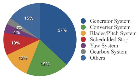
Figure 1.
Percentage of downtime per component for two wind power plants in China.
Recent research work has tried to tackle this problem. The most effective methods are based on purpose-designed CMSs [6], which integrate condition monitoring to the supervisory control and data acquisition (SCADA) systems [1]. However, high deployment cost is the primary limiting factor for existing purpose-designed CMSs. These purpose-designed CMSs have to rely on high-frequency (e.g., 2 kHz for shaft vibration or 20 kHz for gearbox vibration) sensing devices to support wind turbine fault detection with sufficient accuracy. Thus, expensive extra sensing devices are required in this system. Therefore, high deployment costs of purpose-designed CMSs have seriously limited their adoption. Compared with purpose-designed CMSs, there are also some methods that are based on SCADA systems. A SCADA system provides minute-level data sensing resolution, which has been considered inadequate to support accurate fault detection and prediction [6]. These methods usually do not rely on extra expensive devices, hence avoiding additional deployment costs.
This paper first discusses the challenges of using SCADA to support generator fault prediction and diagnosis. It then presents an unsupervised learning method to perform generator fault prediction, remaining useful life (RUL) estimation and fault type diagnosis. Two wind power plants have been adopted in the proposed work. The experimental study demonstrates that the proposed prediction model can provide: (1) sufficient lead time for operators to schedule maintenance activities before generator faults occur and (2) accurate diagnosis of the specific fault types of the wind turbine when faults occur. The contributions of the work are summarized as follows.
- We have conducted an extensive analysis of data (containing SCADA data and status data) collected by SCADA systems. We propose a data preprocessing procedure for the data, which mainly includes four steps: data cleaning, feature selection, feature reduction, and data set balancing. In particular, principal component analysis (PCA) is used to identify suitable features which can capture generator fault changes. The synthetic minority over-sampling technique (SMOTE) is used to tackle the imbalance characteristics of the data set with better accuracy.
- We have developed a solution containing a prediction model and diagnosis model. In the prediction model, the wind turbine generators’ remaining useful life (RUL) is predicted using an unsupervised clustering method. Also, a notion, the anomaly operation index (AOI), is proposed for better visualization of the wind turbine generators developing fault trajectories. We also present a RUL estimation method to predict generator RUL. The diagnosis model is a complementary tool for fault prediction. In the diagnosis model, we compare widely used classifiers and choose the most appropriate classifier for combination with the SMOTE for accurate fault diagnosis.
- The proposed solution has been adopted and evaluated using two wind power plants located in China. Experimental results show that emerging generator faults can be predicted 18 days ahead with about 80% accuracy. In addition, the diagnosis model can be a complementary tool for classifying generator failure types with over 94% accuracy when they occur.
The rest of this paper is organized as follows. Section 2 surveys the related work. Section 3 discusses the challenges for wind turbine generator RUL prediction and fault diagnosis via SCADA systems. Section 4 analyzes the characteristics of the data set that we use and presents the data pre-processing process. In Section 5, we present a solution that integrates a prediction model and diagnosis model for wind turbine generators. Experimental results are presented in Section 6. Finally, we conclude this work in Section 7.
2. Related Work
Many previous studies have conducted fault prediction and diagnosis using SCADA systems. Two comprehensive reviews of existing approaches for fault diagnosis are provided by Lu et al. [2] and Márquez et al. [5]. These methods focused on detecting gearbox faults [7,8,9], blades/pitch faults [10,11], drive train faults [9,10], and main bearings faults [12,13,14].
Often, occurring faults can be detected by monitoring the temperature variation for the major components of wind turbines. Zaher et al. revealed that the increasing temperature of gearbox oil could indicate a fault in the gearbox [7]. They predicted the temperature of gearbox oil using the artificial neural network (ANN) model. The residuals between the model output and the actual signals collected by SCADA system are used to determine whether a fault is present or not. Kusiak et al. identified over-temperature events of bearing faults by capturing the relationship among input signals collected by the SCADA system, in which ANN models were also used [13]. Zhang et al. [14] investigated a wind turbine’s main bearing faults also using the ANN method. Schlechtingen et al. compared the detection efficiency for bearing faults and the stator temperature anomalies using a regression model and an ANN model [12]. Yang et al. mainly focused on detecting incipient wind turbine blades and drive train faults by investigating the correlations among the relevant SCADA data. They provided a suggestive list that maps some relationships of signals collected by SCADA data to a fault [10]. Kusiak et al. explored status data provided by SCADA system to offer fault prediction for most frequent faults on four wind turbines for three months [15]. Although the prediction accuracy of fault category is somewhat lower, their study offered new insights, which help to design fault prediction approaches using status data. Building on top of the previous works, this work: (1) conducted detailed data analysis and feature selection for generator fault diagnosis and prediction; and (2) combined the SCADA data with status data for fault diagnosis.
There are some works that aimed at detecting faults occurring on one subsystem of a generator system. The temperature change was used to indicate a generator ventilation system failure [9]. A hybrid model was developed to detect generator cooling system fault in [16]. Our work is different from these methods in the following aspects. Firstly, this study focuses on the overall generator system, while the works above focused on one subsystem of a generator. Secondly, for the first time, our study proposed a solution which combined generator fault diagnosis and prediction.
3. Challenges
Tackling generator fault prediction and diagnosis via SCADA systems can be viewed as finding faulty generator behaviors that do not conform to expected normal behavior from SCADA data. A straightforward anomaly detection approach, therefore, can be used for the purpose. Unfortunately, such an approach is challenging for several reasons.
The primary challenge in generator fault prediction and diagnosis via SCADA systems is designing a meaningful and actionable data analysis method. Using the method, the normal behavior which encompasses every possible normal operational status for wind turbine generators is modeled. Thus, non-conforming behaviors can be recognized. However, compared with purpose-designed CMSs that collect high-frequency data such as acceleration and acoustic emission, SCADA systems are not initially designed for condition monitoring purposes. As such, they receive only limited and low-frequency signals, e.g., power output, mechanical velocity, and temperature. Therefore, it is challenging to capture incipient faults behaviors from the raw SCADA data without effective data analysis. Nevertheless, SCADA systems provide information which can potentially reveal the normal condition of wind turbines. A power curve has been widely used to detect wind turbine faults. More specifically, the correlation between wind speed and active power output collected by SCADA data is compared against the standard power specification provided by the equipment manufacturer. Figure 2a shows a wind turbine that operates properly. Figure 2b shows a wind turbine that experiences a fault. However, it is difficult to identify the exact cause, or develop fault progression trajectory and perform fault prediction and diagnosis.
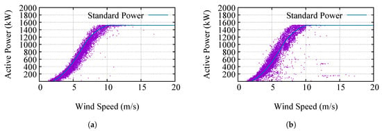
Figure 2.
Power curves of a wind turbine in a normal condition (a) and a developing fault condition (b) with the same sampling resolution.
Variable-speed operation and the stochastic characteristics of aerodynamic load pose another challenge for fault prediction and diagnosis. For instance, the high-speed shaft is one of the main components of the generator system. In general, the higher the wind speed, the higher the load of the shaft. The higher the load, the greater the possibility of fault [2], because the load is acting on the shaft due mainly to the reaction of the contact forces. This reaction force is directly proportional to the torque transferred between the rotor and generator. Shaft torque measurements have been employed for shaft fault detection due to high load [2,17]. Although SCADA systems do not collect shaft torque, we can still use the following equation to derive the torque.
where Q is the torque, P is the generator active power, and is the generator´s rotational speed. However, firstly due to random environmental factors, an instantaneous superior torque may not suggest a fault. Secondly, due to inherent variable-speed operation characteristics of a wind turbine (e.g., the generator´s rated rotational speed is 1800 rpm and the generator´s rotational speed range is 1000 rpm–2000 rpm in this study, Sinovel, Beijing, China), faults are usually not in the form of excessive torque, but in the form of continuous disproportion between wind speed and torque, or wind speed and active power. For instance, a fault occurred in wind turbine number 23 in March 2014. Figure 3a shows the variation of active power with wind speed. Figure 3b illustrates the variation of torque with wind speed. We can infer that the wind turbine may have been experiencing a developing fault in February 2014. The active power and torque of most instances are lower than that of the past months under the same wind speed. However, not all the instances of active power and torque are lower than those of the previous months under the same wind speed. This also suggests that generator degradation is usually an accumulation process (e.g., in days or months) rather than an instantaneous action (e.g., in minutes).
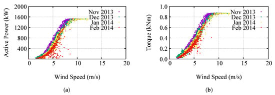
Figure 3.
Active power vs. speed (a) and torque vs. wind speed (b).
Another challenge to implementing generator fault diagnosis is the data set, which is highly imbalanced. A data set is imbalanced if the classes (majority class and minority class) are not approximately equally represented [18]. For fault diagnosis, our goal is building a classifier to distinguish the wind turbines’ fault status and normal status. Each instance in the SCADA data is labeled as fault or normal according to the status data. The intuition is that most of the wind turbines are fault-free most of the time. Thus, normal instances in the data set significantly outnumber the fault instances. Therefore, the data set is imbalanced. We refer to the class containing normal instances as the majority class. Another class is referred to as the minority class. For the two wind power plants that we experimented with, six wind turbines had a generator replacement fault. Table 1 summarizes the instance number in the majority class and minority class. As demonstrated in Table 1, the data set is highly imbalanced with a very small number of minority instances and a large number of majority instances. Our decision system targets the rare but important minority class, which causes the data set imbalance problem.

Table 1.
Data set distribution.
4. Data Description and Pre-Processing
4.1. Data Collection
The SCADA data we used in this study were collected over a period of 18 months at two real-world wind power plants (150 wind turbines). For each turbine, two separate sets of data were provided: SCADA data and status data. Specifically, the SCADA data contain 58 parameters for each turbine with a one-minute interval. The status data provide information on fault status. Table 2 shows the related parameters of each wind turbine in the wind power plants.

Table 2.
Parameters for wind turbines in the two wind power plants.
4.1.1. SCADA Data
The SCADA data we used in this study were collected for every second. For each turbine, 58 parameters were obtained in SCADA data, which are grouped into four categories.
- The condition parameters contain wind speed, wind direction, and ambient temperature, which can determine the power output of wind turbines.
- The health parameters contain main bearing temperature, low-speed shaft temperature, high-speed shaft temperature, and gearbox oil temperature, which can help analyze the health condition of wind turbines.
- The performance parameters contain rotor speed, impeller speed, generator speed and active power, etc., which measure wind turbines´ operational performance.
- The controlling parameters refer to the programmable logic controller code (PLC) state. There are 17 PLC state codes, which are system initialization, system interrupt, system maintenance, system power-generating, etc.
4.1.2. Status Data
The status data provide information on fault status, mainly including five parameters: wind turbine (WT) number, the cause of a fault, the maintenance activities for the fault, the start date for the maintenance, and the end date for the maintenance. Table 3 shows two examples of the status data.

Table 3.
Example of status data collected by supervisory control and data acquisition (SCADA) systems.
4.2. Data Cleaning
4.2.1. Removing Errors
The SCADA data and status data collected by a SCADA system are usually contaminated by errors due to malfunctions in the data collection system. The first step of data cleaning is removing these errors [19]. We can identify errors based on attribute (field) and record type. Table 4 [19] shows the errors for the various cases in this study.

Table 4.
Illustration of errors in SCADA data and status data.
4.2.2. Re-Sampling
After removing the errors, the SCADA data are re-sampled. Since the 10-min sampling interval has been widely adopted in existing SCADA-based fault prediction and diagnosis literature [7,12], we re-sampled the data using the ten-minute interval. All the entries in the re-sampled data are equated every ten minutes. Note that, according to [20], we should guarantee that the data integrity for every minutes minutes is larger than 90%. The following equation defines the data integrity.
where is the number of instances that should be measured in ten minutes (600 instances) by SCADA data, is the number of missing instances, and is the number of instances that contain errors.
4.3. Feature Selection
Since not all features in SCADA data are related to generator faults, we first need to identify the subset of the features collected by the SCADA system that reflects generator operation states. More specifically, the features that allow us to analyze generator faults fall into the first, second, and third categories in Section 4.1.1 [21]. Table 5 summarizes the selected features and potential correlations for generator fault prediction and diagnosis purposes.

Table 5.
Features and reasoning rules for predicting the remaining useful life (RUL) and fault diagnosis of the wind turbine generators.
4.4. Feature Reduction
The features defined in Table 5 are selected based on insights from domain experts. However, these features contain some level of redundancy. For instance, the temperature of low-speed shaft and temperature of high-speed shaft are closely related. Their Pearson correlation coefficient is larger than 0.98. The active power and reactive power are also closely related. Their Pearson correlation coefficient is larger than 0.95. To better describe data, we should combine these similar features into a single feature [22]. Otherwise, the redundancy in the features will affect the model performance [23]. Principle component analysis (PCA) achieves the process of combining the similar features. PCA was proposed by Wold et al. [23], which aimed at transforming the original features into a set of linear combinations. We adopted PCA here to find the optimal combination (i.e., components) of features while accounting for more information of original features. All features in Table 5 are used in subsequent analysis. We restrict the major two components accounting for at least 97.44% of the variance of the input features.
4.5. Data Set Balancing
Handling imbalanced data sets is usually accomplished by generating a balanced data set. There exist two kinds of techniques to balance data sets: under-sampling the majority class technique [24] and over-sampling the minority class technique [25]. An under-sampling technique works by removing some instances in the majority class. This method is prone to discarding potentially useful data [25]. For the case of the support vector machine (SVM) classifier used in this study, removing well inside instances in the majority class has no effect, however removing margin instances may significantly affect the performance of the SVM classifier. In this study, to avoid the removal of potentially useful instances, we use the over-sampling technique to balance the data set. Also, to avoid making exact copies of existing instances in over-sampling techniques, we use the SMOTE [25] to avoid over-fitting. SMOTE works by creating examples so as to balance the data set. More specifically, SMOTE considers the differences between each instance in the minority class and the N nearest neighbors of each instance. First, the SMOTE identifies the N nearest neighbors for each instance in the minority class. Then, the SMOTE chooses N random points along each line segment between the instance and each chosen neighbor. The N random points are the examples. The number of nearest neighbors N determines the amount of the over-sampling. For instance, if the amount of over-sampling needed is , only ten neighbors are randomly chosen. Based on SMOTE [25], the detailed procedure of balancing the optimal subset of features is presented in Algorithm 1. Our implementation currently uses 28 nearest neighbors because the training set will be balanced if the amount of over-sampling is as shown in Section 6.
| Algorithm 1 BalancingFeaturesSpace () |
| Require: Minority class (T is the number of minority class instances) in optimal features subset; Amount of SMOTE (); Number of nearest neighbors . |
| Ensure: synthetic instances in minority class. |
| for each instance in minority class M do |
| Compute nearest neighbors ; |
| while do |
| Randomly choose one neighbor from ; |
| Compute the distance between and ; |
| Generate a random gap (1); |
| Generate a synthetic instance ; |
| ; |
| end while |
| end for |
5. Prediction and Diagnosis Solution
In this work, we propose an integrated prediction and diagnosis solution based on machine learning techniques and statistical techniques via SCADA systems. Figure 4 gives an overview of the proposed solution. The solution consists of two layers: the data layer and decision support layer. The data layer contains the data collected by SCADA systems. The decision support layer includes the process of data pre-processing and two models: the prediction model and diagnosis model. In the prediction model, we first use an unsupervised learning method to cluster the operational state of generators so as to estimate the RUL of a generator. The diagnosis model implements the mapping from feature space to state space for a generator through supervised classification method. The prediction is more difficult than diagnosis since its accuracy is subjected to the stochastic process of failure events that are yet to occur. Nevertheless, the prediction cannot completely replace diagnosis since diagnosis can be a complementary tool for providing maintenance decision support in the case of unsuccessful prediction [26]. The following subsections describe the details of prediction and diagnosis models.
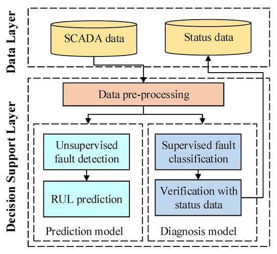
Figure 4.
Overview of the integrated wind turbine generator fault prediction and diagnosis solution.
5.1. Prediction Model
The prediction model focuses on capturing a generator’s unhealthy operational state before a fault occurs, and further predicts the generator’s remaining useful life (RUL). A generator’s unhealthy state refers to the long degradation process with respect to a developing fault.
As discussed in the earlier work [21], there exists a pure intuition that most of the generators function most of the time healthily, and faults rarely occur. For the top three components output from the process of data-preprocessing, the largest and densest cluster exists. Most of the instances that reflect a generator’s healthy operational state belong to this cluster. Other instances that reflect a generator’s unhealthy state do not belong to this cluster. Thus, density-based spatial clustering of applications with the noise (DBScan) method that relies on the formation of clustering by the density of instances is appropriate. According to the above intuition, we assign instances which belong to the densest and largest cluster as healthy instances. Instances that do not belong to the cluster or noise can be considered as unhealthy instances. Generator state change from healthy to unhealthy is an accumulation process rather than an instantaneous process. Therefore, an instantaneous unhealthy state may not suggest a fault due to random environmental factors. The continuous unhealthy state can indicate a developing or developed fault. Thus, the anomaly operation index () is proposed to measure a wind turbine’s performance over a period of historical time t [21]. is defined as Equation 3, which reflects the proportion of unhealthy instances to all instances during a time period of t.
where is the number of instances during period t, and is the number of instances that belong to the largest and densest cluster. AOI can be an indicator of a wind turbine generator´s performance for a period. A larger AOI indicates a higher possibility of wind turbine performance degradation over a given time. At last, we should determine how much time is left before a fault will occur if an AOI value is given. The step is also called RUL estimation. RUL is defined as the conditional random variable [26].
where denotes the random variable of time to a fault, is the current age, and is the generator condition profile up to the current time t. Overall, the key steps of the prediction model are summarized as follows:
step 1: Cluster the instances with top two components derived from the data pre-processing process using the DBScan algorithm.
step 2: Generate during a time period of t.
step 3: Determine the characteristics of combining the autoregressive integrated moving average model (ARIMA) model [27].
step 4: Obtain the current for a generator.
Algorithm 2 presents the detailed procedure of predicting a generator’s RUL.
| Algorithm 2 Prediction () |
| Require: the instances set over a period of time ; the smooth window ; the boundary from normal to abnormal ; weight related to actual remaining useful life at any time slot for a normal wind turbine. |
| Ensure: remaining useful life at time t. |
| Cluster the set I. |
| Initialize the anomaly index container ; |
| for each do |
| Calculate instance number in the largest and densest cluster for a time period over to . |
| ; |
| end for |
| Initialize a counter container ; |
| for each element in z do |
| if then |
| ; |
| else |
| ; |
| end if |
| end for |
| return ; |
5.2. Diagnosis Model
To use SCADA systems to monitor the operation state of generators, mapping from the feature space to the state space (i.e., [features]→{fault, normal}) is required. A classifier can accomplish this process. Although previous studies suggest some classifiers [22,28], including support vector machine (SVM), k-nearest neighbors (KNN), artificial neural network (ANN) and naive Bayesian, we still need a best-suited classifier that can distinguish the different states of wind turbine generators.
5.2.1. Support Vector Machine
SVM is widely used for classification and regression purposes [29]. When SVM is adopted for classification, its excellent generalization ability has been demonstrated [30]. This ability can be shown through building a model so as to separate marked inputs by a gap that is as wide as possible. The model categorizes instances that are to be classified into different classes.
For a given instance , n is the number of features and t is the time. Let be the state (class) at time t and , where stands for the fault state and represents the normal state. For the binary classification problem, the decision function can be described as [31]:
where are support vectors, and is a kernel function that maps the data to a higher-dimensional space. In our later experiments, we conduct classifying with the LIBSVM library provided by Chang and Lin for the wind turbine generator state classification [32].
5.2.2. K-Nearest Neighbor
KNN is a non-parametric machine learning algorithm, and it is usually used for classification. KNN works first by storing all distances among marked instances and the instances’ labels [28,33]. Then, KNN realizes a classification for each instance by using a majority vote of its k neighbors [33]. That is, each instance to be predicted is assigned to the class that is most common amongst its k most similar neighbors. For instance, given an instance , KNN finds the k most nearest instances to in the training set. In this study, we use the Euclidean distance, , to measure the distance metric between two instances and . In the later experiments, we empirically determined .
5.2.3. Artificial Neural Network
The ANN is also widely used for classification and regression problems [28]. In this study, we use ANN for classification purposes. A three-layer neural network model is adopted here, and we use the back propagation algorithm to train the model. In the training process, features instances are adopted as an input layer. We empirically determine five hidden neurons as a hidden layer. The bipolar sigmoid function is used as an activation function to realize classification. In the testing phase, each instance that is to be classified is inputted into the trained network to obtain the prediction output.
5.2.4. Naive Bayesian
The naive Bayesian classifier is based on the assumption that all classes have conditional independence [28]. The naive Bayesian classifier performs calculation of the posterior probability that a feature x belongs to a given class c, . More specifically, is defined as the following equation:
where is the prior probability of class c. is the likelihood probability that a feature x belongs to a given class c. is the prior probability of feature x.
6. Experiments and Results
In this section, we evaluate the proposed generator fault prediction and diagnosis method. First, we assess the overall prediction performance. We then implement the SVM, ANN, KNN, and naive Bayesian classifiers to identify generator fault status. After evaluating the performance of the different classifiers, the SMOTE is combined with the different classifiers to balance the data set. Thus, the best classifier is chosen based on the performance evaluation of these classifiers.
6.1. Evaluation Metrics
6.1.1. Prediction Performance Metrics
To evaluate the accuracy of RUL prediction, the prediction accuracy for a certain prediction step t is calculated using Equation (7).
where is estimated RUL at t-th day ahead and is actual RUL at t-th day ahead.
6.1.2. Diagnosis Performance Metrics
To evaluate the accuracy of the proposed fault diagnosis method, we refer to a correctly classified instance in the minority class as a true positive classification (TP). A true negative classification (TN) relates to a properly classified instance in the majority class. In addition, false positive (FP) and false negative classifications (FN) correspond to incorrect classification for instances in the minority class and majority class, respectively.
The classification accuracy gives a measure of how often the classification is correct. For a classifier, it is thus computed as the ratio of the number of correct classification to the total number of classification. Specifically, Equation (8) defines the classification accuracy.
However, the classification accuracy may only partially describe a classifier’s performance because it does not consider the misclassification cost. On the one hand, a true positive () increases the efficiency of fault diagnosis, which means the generator fault status can be revealed correctly. True positive rate (TPR) in Equation (9) denotes the frequency.
On the other hand, a true negative () increases the reliability of fault diagnosis, which means the normal status can be identified correctly. We use true negative rate (TNR) to quantify the frequency of such classifications.
The ideal result is that all fault instances are classified correctly, and no normal instances are misclassified as faults. The larger the ACC, TPR, and TNR, the better the detection results.
6.2. Overall Performance
6.2.1. Prediction Performance
The performance degradation of wind turbines lasted for about 44 days until a fault occurred, and similar phenomenon is observed on other wind turbines [21]. Therefore, we use predictions at , , , and days ahead as baselines to predict a fault, respectively. Figure 5a shows the prediction accuracy of RUL for the five turbines experiencing generator fault. As shown in Figure 5a, there is a general trend that the average prediction accuracy improves as the required repair and maintenance lead time decreases. Although there is a slight fluctuation caused by stochastic of wind turbines operation in the curve, the overall trend is clear. Figure 5b shows the mean accuracy. As shown in Figure 5b, the fewer days used to predict in advance, the higher the accuracy. More specifically, the average prediction accuracy is about 80% if the required repair and maintenance lead-time is 18 days ahead.
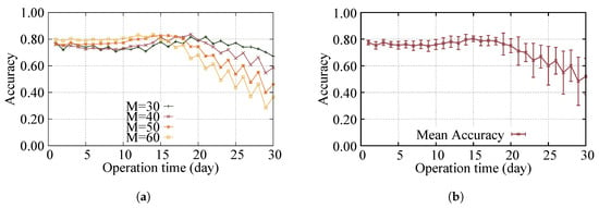
Figure 5.
Prediction accuracy of RUL with different days ahead (a); Mean prediction accuracy of RUL (b).
6.2.2. Diagnosis Performance
This subsection consists of three experiments. In the first experiment, we examine the diagnosis performance of the underlying behavior of each of the aforementioned classifiers: ANN, KNN, SVM, and naive Bayesian. Then, we discuss whether these classifiers are suitable for generator fault diagnosis. In the second experiment, we evaluate the diagnosis performance of each classifier combined with the SMOTE. We also assess the performance of each classifier regarding the area under the curve (AUC) of receiver operating characteristic (ROC) curve. In the last experiment, we discuss the impact of SMOTE and choose the most suitable over-sampling degree N.
To make sure that the classifier is not over-fitting the data, we divide the data into training and test sets. We select wind turbine number 10 randomly as the training set and other turbines as the test set.
Table 6 shows the accuracy of different classifiers. The best performance of different classifiers is indicated in bold print. As Table 6 demonstrates, overall, there is no best classifier for maximizing , and simultaneously. The main reason is that the different classifiers are suitable for various scenarios. The KNN classifier performs best in identifying , as the classifier is dedicated to finding the nearest neighbors. Negative instances in the data set are very dense, so KNN has a good ability for identifying . The ANN classifier performs best in identifying and , as it is based on the data characteristics of finding the non-linear relationship between the feature and the corresponding status. On the other hand, the highest only achieves an accuracy of 71.15%. This is mainly because the data set is imbalanced and instances in minority class are far fewer than the number of instances in majority class. Therefore, is low regardless of classifiers.

Table 6.
Classification accuracy for different algorithms before the training set is balanced. ANN: artificial neural network; KNN: k-nearest neighbors; SVM: support vector machine; TPR: true positive rate; TNR: true negative rate; ACC: classification accuracy.
After using the SMOTE, increases significantly for an SVM classifier if the data set is balanced. The highest is 96.34% if the minority class is over-sampled by SMOTE at of its original size, where N is 28. When N is up to 28, the majority and minority class are approximately equally represented in the training set, that is the training set is balanced. Table 7 shows the accuracy of different classifiers when N is 28. As shown in Table 7, the SVM classifier works best in identifying , but the KNN classifier works best in recognizing and achieving the highest . Therefore, we still cannot choose the best classifier from Table 7.

Table 7.
Classification accuracy for different algorithms after the training set is balanced.
For a class imbalance problem, it is true that a good performance can be achieved by always reporting the largest state. As shown in Table 6, all s are larger than s. Figure 6c shows that increases significantly for the SVM classifier after using the SMOTE. and decrease slightly as N increases, while increases significantly. Figure 6a,b,d show that there are no such results for other classifiers.
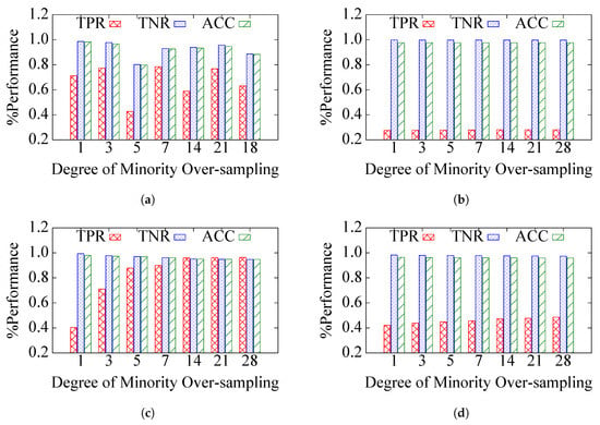
Figure 6.
Different classifiers: (a) the ANN classifier; (b) the KNN classifier; (c) the SVM classifier and (d) the Bayes classifier.
Since the SVM classifier clearly dominates others over the entire performance space, we use the AUC to determine the best classifier for our application. ROC is depicted in the scenarios that minority class is over-sampled by the SMOTE at of its original size, where N is 1, 3, 5, 7, 14 and 28, respectively. Figure 7 shows the AUC scores for different classifiers. From Figure 7, we observe that SVM compares favorably to all the other classifiers regarding AUC. Thus, in the later experiments, we will choose the SVM classifier as the most suitable classifier.
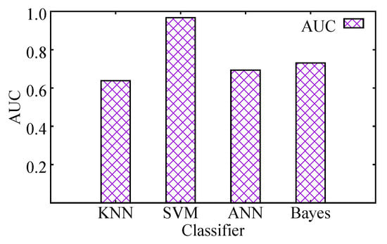
Figure 7.
Average prediction accuracy of RUL for six wind turbines. AUC: area under the curve.
Finally, we analyze the performance of the SVM classifier under the different degrees of over-sampling. The minority class is over-sampled by the SMOTE at of its original size, where N is 1, 3, 5, 7, 14, 21 and 28, respectively. As shown in Figure 6c, ACC and TNR decrease slightly as N increases, and they are approximately equal at the same N. TPR, however, increases as N increases significantly. This is because the classifier will pay more attention to the instances in the minority as the degree of these instances over-sampling increases. Figure 8 shows the corresponding ROC curve. In particular, TPR increases mostly when N varies from 1 to 7 because support vectors increase significantly in the early stage of instances in the minority over-sampling. When N is larger than 14, the decrease of ACC and TNR and the increase of TPR tend to be stable because the data set tends to balance. Thus, we can choose to conduct the diagnosis experiments.
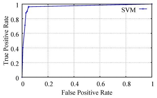
Figure 8.
ROC curve for the SVM classifier under the different degrees of minority over-sampling. ROC: receiver operating characteristic.
7. Conclusions
This paper presents a solution for wind turbine generator RUL prediction and fault diagnosis, which has been adopted by two real-world wind power plants. The experimental study shows that, using the proposed method, wind turbine generator RUL can be predicted with about an 80% accuracy 18 days ahead. The generator faults can be diagnosed with a 94% accuracy when they occur. Compared with purpose-built CMSs equipped with special high-frequency data sensing hardware, the proposed method is cost-efficient, as it relies solely on the information provided by widely available SCADA system and does not require additional installation of purpose-built data sensing equipment for wind power plants.
Acknowledgments
This work was supported by National Natural Science Foundation of China under Grant No. 61233016.
Author Contributions
Yingying Zhao, Dongsheng Li and Ao Dong carried out of the work present here; Dahai Kang contributed data set and analysis tools; Dongsheng Li, Qin Lv and Li Shang supervised the proposed research.
Conflicts of Interest
The authors declare no conflict of interest.
References
- Pérez, J.M.P.; Márquez, F.P.G.; Tobias, A.; Papaelias, M. Wind turbine reliability analysis. Renew. Sustain. Energy Rev. 2013, 23, 463–472. [Google Scholar] [CrossRef]
- Lu, B.; Li, Y.; Wu, X.; Yang, Z. A review of recent advances in wind turbine condition monitoring and fault diagnosis. In Proceedings of the Power Electronics and Machines in Wind Applications, Lincoln, NE, USA, 24–26 June 2009; pp. 1–7. [Google Scholar]
- Tavner, P.J.; Xiang, J.; Spinato, F. Reliability analysis for wind turbines. Wind Energy 2007, 10, 1–18. [Google Scholar] [CrossRef]
- McMillan, D.; Ault, G.W. Quantification of condition monitoring benefit for offshore wind turbines. Wind Eng. 2007, 31, 267–285. [Google Scholar] [CrossRef]
- Márquez, F.P.G.; Tobias, A.M.; Pérez, J.M.P.; Papaelias, M. Condition monitoring of wind turbines: Techniques and methods. Renew. Energy 2012, 46, 169–178. [Google Scholar] [CrossRef]
- Yang, W.; Tavner, P.J.; Crabtree, C.J.; Feng, Y.; Qiu, Y. Wind turbine condition monitoring: Technical and commercial challenges. Wind Energy 2014, 17, 673–693. [Google Scholar] [CrossRef]
- Zaher, A.; McArthur, S.D.J.; Infield, D.G.; Patel, Y. Online wind turbine fault detection through automated SCADA data analysis. Wind Energy 2009, 12, 574–593. [Google Scholar] [CrossRef]
- Kim, K.; Parthasarathy, G.; Uluyol, O.; Foslien, W.; Sheng, S.; Fleming, P. Use of SCADA data for failure detection in wind turbines. In Proceedings of the American Society of Mechanical Engineers (ASME) 2011 5th International Conference on Energy Sustainability, Washington, DC, USA, 7–10 August 2011; pp. 2071–2079. [Google Scholar]
- Qiu, Y.; Feng, Y.; Sun, J.; Zhang, W.; Infield, D. Applying thermophysics for wind turbine drivetrain fault diagnosis using SCADA data. IET Renew. Power Gener. 2016, 10, 661–668. [Google Scholar] [CrossRef]
- Yang, W.; Court, R.; Jiang, J. Wind turbine condition monitoring by the approach of SCADA data analysis. Renew. Energy 2013, 53, 365–376. [Google Scholar] [CrossRef]
- Gill, S.; Stephen, B.; Galloway, S. Wind turbine condition assessment through power curve copula modeling. IEEE Trans. Sustain. Energy 2012, 3, 94–101. [Google Scholar] [CrossRef]
- Schlechtingen, M.; Santos, I.F. Comparative analysis of neural network and regression based condition monitoring approaches for wind turbine fault detection. Mech. Syst. Signal Process. 2011, 25, 849–1875. [Google Scholar] [CrossRef]
- Kusiak, A.; Verma, A. Analyzing bearing faults in wind turbines: A data-mining approach. Renew. Energy 2012, 48, 110–116. [Google Scholar] [CrossRef]
- Zhang, Z.Y.; Wang, K.S. Wind turbine fault detection based on SCADA data analysis using ANN. Adv. Manuf. 2014, 2, 70–78. [Google Scholar] [CrossRef]
- Kusiak, A.; Li, W. The prediction and diagnosis of wind turbine faults. Renew. Energy 2011, 36, 16–23. [Google Scholar] [CrossRef]
- Borchersen, A.B.; Kinnaert, M. Model-based fault detection for generator cooling system in wind turbines using SCADA data. Wind Energy 2016, 19, 593–606. [Google Scholar] [CrossRef]
- Gray, C.S.; Watson, S.J. Physics of failure approach to wind turbine condition based maintenance. Wind Energy 2010, 13, 395–405. [Google Scholar] [CrossRef]
- Kotsiantis, S.; Kanellopoulos, D.; Pintelas, P. Handling imbalanced datasets: A review. GESTS Int. Trans. Comput. Sci. Eng. 2006, 30, 25–36. [Google Scholar]
- Rahm, E.; Do, H.H. Data cleaning: Problems and current approaches. IEEE Data Eng. Bull. 2000, 23, 3–13. [Google Scholar]
- General Administration of Quality Supervision, Inspection and Quarantine of the People’s Republic of China GB/T18710. Methodology of Wind Energy Resource Assessment for Wind Farm; Standards Press of China: Beijing, China, 2002.
- Zhao, Y.; Li, D.; Dong, A.; Lin, J.; Kang, D.; Shang, L. Fault prognosis of wind turbine generator using SCADA data. In Proceedings of the North American Power Symposium (NAPS), Denver, CO, USA, 18–20 September 2016; pp. 1–6. [Google Scholar]
- Kleiminger, W.; Beckel, C.; Santini, S. Household occupancy monitoring using electricity meters. In Proceedings of the 2015 ACM International Joint Conference on Pervasive and Ubiquitous Computing, Osaka, Japan, 7–11 September 2015; pp. 975–986. [Google Scholar]
- Wold, S.; Esbensen, K.; Geladi, P. Principal component analysis. Chemom. Intell. Lab. Syst. 1987, 2, 37–52. [Google Scholar] [CrossRef]
- Ling, C.X.; Li, C. Data mining for direct marketing: Problems and solutions. In Proceedings of the Fourth International Conference on Knowledge Discovery and Data Mining, New York, NY, USA, 27–31 August 1998; pp. 73–79. [Google Scholar]
- Chawla, N.V.; Bowyer, K.W.; Hall, L.O.; Kegelmeyer, W.P. SMOTE: Synthetic minority over-sampling technique. J. Artif. Intell. Res. 2002, 16, 321–357. [Google Scholar]
- Jardine, A.K.; Lin, D.; Banjevic, D. A review on machinery diagnostics and prognostics implementing condition-based maintenance. Mech. Syst. Signal Process. 2006, 20, 1483–1510. [Google Scholar] [CrossRef]
- Chen, P.; Pedersen, T.; Bak-Jensen, B.; Chen, Z. ARIMA-based time series model of stochastic wind power generation. IEEE Trans. Power Syst. 2010, 25, 667–676. [Google Scholar] [CrossRef]
- Chandola, V.; Banerjee, A.; Kumar, V. Anomaly detection: A survey. ACM Comput. Surv. (CSUR) 2009, 41. [Google Scholar] [CrossRef]
- Suykens, J.A.; Vandewalle, J. Least squares support vector machine classifiers. Neural Process. Lett. 1999, 9, 293–300. [Google Scholar] [CrossRef]
- Kim, H.E.; Tan, A.C.; Mathew, J.; Choi, B.K. Bearing fault prognosis based on health state probability estimation. Expert Syst. Appl. 2012, 39, 5200–5213. [Google Scholar] [CrossRef]
- Burges, C.J. A tutorial on support vector machines for pattern recognition. Data Min. Knowl. Discov. 1998, 2, 121–167. [Google Scholar] [CrossRef]
- Chang, C.C.; Lin, C.J. LIBSVM: A library for support vector machines. ACM Trans. Intell. Syst. Technol. 2011, 2. [Google Scholar] [CrossRef]
- Sinapov, J.; Wiemer, M.; Stoytchev, A. Interactive learning of the acoustic properties of household objects. In Proceedings of the IEEE International Conference on Robotics and Automation, Kobe, Japan, 12–17 May 2009; pp. 2518–2524. [Google Scholar]
© 2017 by the authors. Licensee MDPI, Basel, Switzerland. This article is an open access article distributed under the terms and conditions of the Creative Commons Attribution (CC BY) license (http://creativecommons.org/licenses/by/4.0/).