Impact of Firms’ Observation Network on the Carbon Market

Abstract

Given the important role of the carbon market in fighting against global warming, the impact of information on the efficiency of the scheme is a critical issue for both its designers and the central authority. At least two aspects of information are worthy of attention. First is the incompleteness of information, with which the firms make decisions to minimize their abatement cost and maximize their profit. Second is the mechanism of information transmission. Based on an agent-based framework we established in our previous work, we explicitly depicted the first aspect and analysed its impact on firms’ decision-making and consequent market results. In this paper, we focus on the second aspect, transmission mechanism of information, which is depicted as an observation network among firms. The basis in reality is that the firms in the carbon market are usually from different industries or areas, and it is relatively easier to observe the conditions of firms from the same industry or area, corresponding to neighbours in the network. Four scenarios are considered, including no network, regular network, random network, and small-world network. We find that the existence of an observation network has a significant influence on the market results.

1. Introduction

Facing the challenge of global warming and the pressure of carbon emission reduction, the scheme of emission trading has been regarded as a flagship policy instrument. Numerous studies have been conducted on the design [1,2] of this scheme. Additionally, the impact of the scheme has also been evaluated, including is impact on the macro economy [3,4,5], economic performance of sectors or firms [6,7], and financial performance of firms [8,9]. However, several aspects of complexity have pushed traditional equilibrium-based models to their limit, including the dynamic aspect of market evolution, bounded rationality, heterogeneity, and incomplete information of the firms in the market. So, in our previous work [10], we establish an agent-based framework for the simulation of the carbon market, considering the four aspects of complexity above. Within this framework, firms’ incomplete information is explicitly modelled as an attribute “Eyesight” of firms $\left(EY{E}_i\right)$, representing the limited number of other firms that a firm can observe when forming its forecast of the allowance price. Then, we analyse its impact on firms’ decision-making and consequent market results. We find that there is a statistically significant impact of firms’ $EY{E}_i$ on the market results: when $EY{E}_i$ rises, the average allowance price rises, and firms’ total adoptions of low-carbon technologies decreases. Furthermore, we find that the social average abatement cost decreases with rising $EY{E}_i$, which indicates a higher efficiency of the carbon emission trading scheme. This is because with more information, more inefficient adoptions of low-carbon technologies are avoided.

Apart from the incompleteness of information, another aspect worthy of attention is the transmission mechanism, which is the main focus of this paper. It is depicted as an observation network among firms. The basis in reality is that the firms in the carbon market are usually from different industries or areas, and it is easier to observe the conditions of firms from the same industry or area. These conditions include production quantity, energy intensity, adoption of low-carbon technologies, etc. Neighbouring firms in the observation network correspond to firms from the same industry or area. As far as we know, no study has yet analysed the influence of firms’ observation network on the carbon market, neither theoretically nor empirically. However, in a broader view of network science, the influence of the observation or interaction network among agents has been a common issue in the studies of financial markets [11,12,13] and technology diffusion processes [14,15,16]. Correspondingly, the agent-based model is one of the major tools for a relevant analysis. Both of these strands of studies provide referential significance. In this paper, we attempt to simulate the influence of firms’ observation network in the carbon market based on an agent-based model.

In our model, the introduction of observation is related to the formation of firms’ forecasts of the allowance price. Firms form their forecast based on two aspects of information. First, a firm (e.g., firm i) forms its fundamental estimate of the allowance price based on conditions of $EY{E}_i$ neighbour firms that it can observe. By observing the other $EY{E}_i$ firms’ condition, firm i can calculate a fundamental estimate of the allowance price from the equilibrium perspective based on three aspects of information. The first is expected total emission of these $EY{E}_i$ firms, which is calculated based on their historical emission, total production in the rest periods of the abatement phase, and current energy intensity. The second is current holdings of emission allowance of these $EY{E}_i$ firms. The third is the marginal abatement cost curve (MACC) of these $EY{E}_i$ firms, which is calculated based on their available low-carbon technologies, and the calculation method is introduced in Section 2.2. The total allowance gap of these $EY{E}_i$ firms can be calculated based on the first two aspects of information. Then, the fundamental estimate of the allowance price can be calculated with MACC combined. Second, firm i calculates the moving average of the allowance price, which represents the technical aspect of information. Finally, firm i’s forecast of the allowance price is a combination of both fundamental and technical information. This forecast serves as a uniform benchmark for firm i to coordinate its multiple abatement-oriented decisions, to minimize its abatement cost and maximize its profit. As a result, the existence of an observation network among firms can influence firms’ forecasts of the allowance price through fundamental aspects of information, as well as their abatement-oriented decisions and the consequent market results.

Regarding the observation network, four scenarios are considered in this paper, including “no network”, “regular network”, “random network”, and “small-world network”. The reason for choosing these four kinds of network as scenarios is that their average $EY{E}_i$ can be controlled equal, which guarantees the comparability among different networks. The “no network” scenario serves as the base scenario in the analysis. Based on the simulation results, we find that the existence of an observation network has a significant influence on the market results, including the allowance price and trading volume in the carbon market, product price and production in the output market, and firms’ total adoption of low-carbon technologies. While there is no significant difference among the three scenarios with the observation network, above all, when the observation network exists, the social average abatement cost increases with firms’ average $EY{E}_i$ rising, which indicates an efficiency loss with increasing information. This is because the existence of an observation network among firms delays the transmission of information, which leads to higher revenue loss in the output market when the average $EY{E}_i$ of firms rises.

This paper is structured as follows: Section 2 presents a brief introduction of our model. A detailed introduction can be found in our previous work [10]. Section 3 introduces settings of the simulation scenarios, and simulation results are shown and discussed in Section 4. Finally, conclusions are given in Section 5.

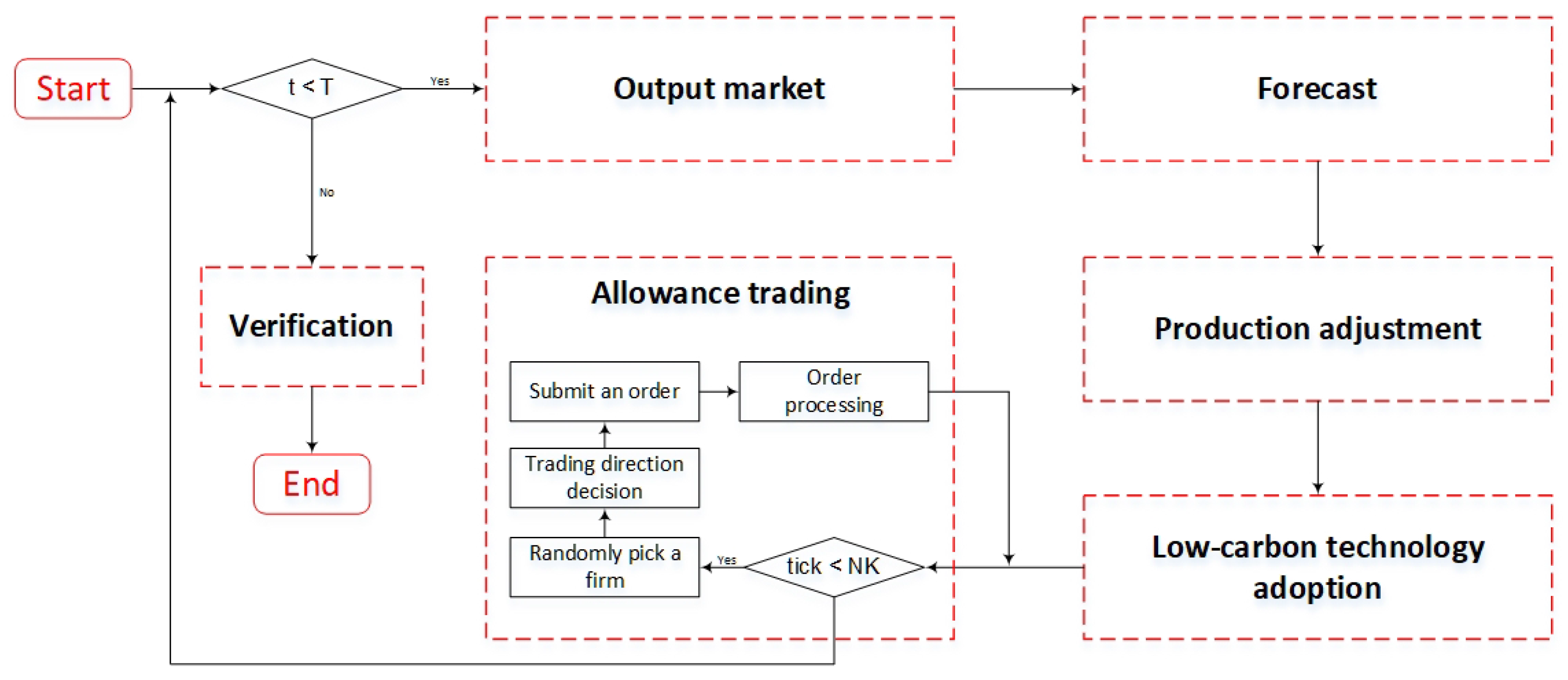
2. Model

2.1. Model Structure

This model simulates an abatement phase with T periods and each period is denoted by t. There are $NA$ agents, representing the target firms, in the carbon market, who compete with each other in both of the output and the carbon markets. All firms share a common goal, which is to maximize their total profit. However, given the abatement pressure, firms need to coordinate three abatement-oriented options, including production adjustment, low-carbon technology adoption, and allowance trading. By the end of the abatement phase, firms’ total emissions of CO${}_2$ are verified, and those who emit more than the holdings of allowance must pay a high fine for each ton of excess emission. In order to characterize this whole process, we introduce a complex time frame in this model.

As shown in Figure 1, in each period t, corresponding to a day in the real world, agents first make their decisions of production quantity, which is recorded together with the amount of induced emission of CO${}_2$ under their condition of energy intensity. The price of the output is calculated based on a linear market demand curve, which is $P_t^p=A-B\times {\sum }_{i=1}^{NA}{q}_t^i$. Then, the agents go through the forecast process and form their forecast of the allowance price, which serves as a uniform benchmark for agents to coordinate three abatement-oriented options, including production adjustment, low-carbon technology adoption, and allowance trading. The trading process in the carbon market is organized based on a continuous double auction mechanism.

2.2. Low-Carbon Technology and Marginal Abatement Cost Curve

There are $NT$ low-carbon technologies considered in this model. Each of them is modelled as three parameters, including adoption cost coefficient $\left(I{C}_j\right)$, operating and maintenance cost coefficient $\left(OM{C}_j\right)$, and energy-saving coefficient $\left(E{S}_j\right)$. However, since different agents have different attitudes toward risk (which are depicted by heterogeneous values of their payback period, $P{B}_i$), the average abatement cost of a technology j for agent i is calculated as follows:

$$\begin{array}{c}\hfill {ac}_t^{i,j}=\frac{{IC}_j+{\sum }_{y=1}^{{PB}_i}\frac{{OMC}_j-{ES}_j\times P^e}{{\left(1+r_f\right)}^y}}{{\sum }_{y=1}^{{PB}_i}{ES}_j\times EF}\end{array}$$

(1)

where $r_f$ is the risk-free rate of return, $P^e$ is the price of energy, and $EF$ is the emission of each unit of energy utilization. Furthermore, based on the estimation of agent i’s production in the remaining periods of the abatement phase, denoted by $Q_t^i$, potential abatement of technology j for agent i in period t is calculated as $A_t^{i,j}=E{S}_j\times Q_t^i\times EF$. Thus, based on the calculation of ${ac}_t^{i,j}$ and $A_t^{i,j}$ for all available low-carbon technology options of agent i, a marginal abatement cost curve (MACC) for agent i or a group of agents can be calculated. It is worth noting that unlike the MACCs in previous work by Baker et al. [17] and Bauman et al. [18], in which the abatement cost is essentially resulted from production reduction and factor substitution, the MACC in our model follows the idea of Li and Zhu [19], and it explicitly reflects the cost and abatement potential of multiple low-carbon technologies from a bottom-up perspective.

2.3. Agents

In this model, agents can be abstracted as collections of attributes and behavioural functions. The attributes include their scale ($Q_{last}^i$, represents agent i’s total production in the last year), initial adoptions of low carbon technology $\left(IT{A}_i\right)$, payback period ($P{B}_i$, represents agent i’s attitude toward risk; a lower $P{B}_i$ indicates relatively higher risk-aversion), “eyesight” ($EY{E}_i$), probability of altering forecast of allowance ($Pr{F}_i$) or production quantity ($Pr{A}_i$), etc. Concerning the behavioural functions, each agent has three abatement-oriented options: production adjustment, low-carbon technology adoption, and allowance trading. However, in order to coordinate these three options, agents first need to form their forecast of the allowance price, which serves as a uniform benchmark for comparison.

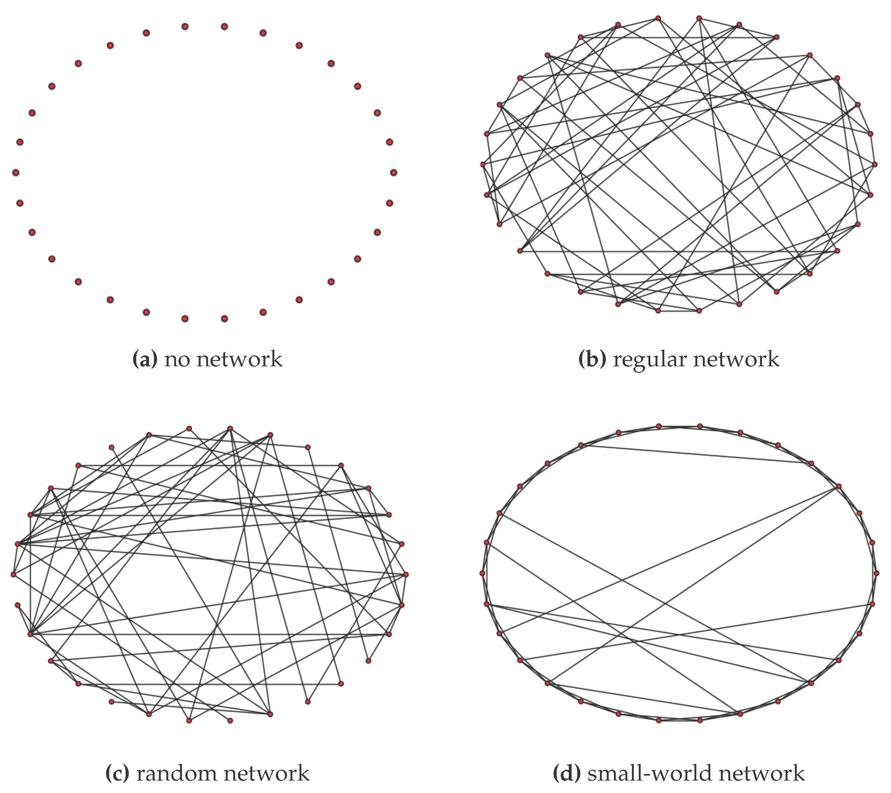
2.3.1. Observation Network and Forecast

In each period, agent i has a probability of $Pr{F}_i$ of adjusting its forecast of the allowance price. As introduced in Section 1, when forming the forecast, agents combine two aspects of information. First is the fundamental aspect of information, which is detailed information of $EY{E}_i$ other agents, including their production quantity, energy intensity, historical emissions, allowance in hand, available low-carbon technology options, etc. Second is the technical aspect of information, which is the moving average of the allowance price. The technical aspect of information is the same for all agents, while the fundamental aspects of information are different, depending on how the observation network is established. Four scenarios are considered in this paper, including no network, regular network, random network, and small-world network, as shown in Figure 2.

For the “no network” scenario, agent i randomly observes $EY{E}_i$ other agents in each period t, and forms its forecast of the allowance price. Then in period $t+1$, agent i forgets this information, and randomly observes another group of agents, and forms its forecast of the allowance price. Thus, in the “no network” scenario, by observing conditions of others, the agents get “limited but global” information (in the “no network” scenario, though agent i can only observe a limited number of other agents in each period t; however, since all other agents can be randomly observed by agent i, we say agent i has “limited but global” information), while in the other three scenarios, the observation network is set before the abatement phase, and the observation relationship between two agents is mutual and constant. Thus, by observing others, the agents in these three scenarios get “limited and local” information (compared with the “no network” scenario, since agent i in these three scenarios can only observe a constant group of neighbour agents, we say agent i has “limited and local” information). The regular network is a kind of network in which each node has the same degree. While in the random network, some links are created randomly. The small-world network was initially introduced to describe the transition from a regular network to a random network. The generating algorithm of three networks can be found in the work by Albert and Barabási [20], and Watts and Strogatz [21]. The comparability among the four networks is established on the basis of a common average degree of nodes; i.e., the average $EY{E}_i$ of agents in the network.

2.3.2. Abatement-Oriented Decisions

Based on the forecast of the allowance price, agent i coordinates its three abatement-oriented options by making three decisions: production adjustment, adoption of low-carbon technologies, and allowance trading in the carbon market. However, since hundreds or even thousands of agents have to coordinate these three options along a dynamic process which contains great uncertainty, their behaviours would inevitably reflect properties of bounded rationality, as they lack sufficient time and information to make decisions. Thus, following the work by Gigerenzer [22], we assume that agents make decisions based on a series of fast and frugal heuristics; i.e., rules of thumb (for simplicity, here we provide a brief introduction of these rules, and a detailed introduction of each rule can be found in our previous work [10]).

1.

Production Adjustment Decision

In each period, agent i has a probability of $Pr{A}_i$ of adjusting its daily production. We introduce a probability $\left({\beta }_t^i\right)$ to characterize agent i’s propensity to adjust its production coefficient $\left({\theta }_t^i\right)$ (Agent i’s daily production is $q_t^i={\theta }_t^i\times Q_{last}^i/T$, and ${\theta }_0^i$ is set to 1, indicating that agent i’s initial daily production was equal to its average daily production in the last year. Then, during the abatement phase, when agent i wants to reduce its production, we let ${\theta }_{t+1}^i={\theta }_t^i-\delta$. In turn, when agent i decides to increase its production, we let ${\theta }_{t+1}^i={\theta }_t^i+\delta$. Here, $\delta$ is an exogenous parameter.). When agent i’s profit of unit emission from the output market $\left(cp{a}_t^i\right)$ (Here the emission allowance is treated as a production factor. Suppose that the product price is $P_t^p$ per ton, and the production cost is $c_i$ per ton. The energy intensity of agent i is ${\rho }_t^i$. The emission factor of the energy is $EF$. Then, profit of unit emission for agent i is calculated as $cp{a}_t^i=\left(P_t^p-c_i\right)/\left({\rho }_t^i\times EF\right)$.) is higher than a benchmark price $\left(bm{p}_t^i\right)$ (Here, $bm{p}_t^i$ is a benchmark price for agent i to make production decision, and it is calculated as $bm{p}_t^i={pfm}_t^i\times pr{o}_i^1$. ${pro}_i^k(k=1,2,3)$ are agent i’s three behavioural parameters related to its production decision. A detailed explanation of the behavioural parameters can be found in the Appendix of [10].), it might increase its production, and the probability is calculated as ${\beta }_t^i={\left(cp{a}_t^i/{bmp}_t^i-1\right)}^{{pro}_i^2}$. When agent i’s profit of unit emission from the output market $\left(cp{a}_t^i\right)$ is lower than a benchmark price $\left(bm{p}_t^i\right)$, it might decrease its production and the probability is calculated as ${\beta }_t^i={\left({bmp}_t^i/{cpa}_t^i-1\right)}^{{pro}_i^3}$.

2.

Low-Carbon Technology Adoption Decision

For simplicity, we assume that in each period t, agent i only considers the adoption of the available low-carbon technology with the lowest average abatement cost. A probability $\left({\gamma }_t^i\right)$ is used to characterize its propensity to adopt this technology. Reasonably, we assume that ${\gamma }_t^i$ is related to four factors: (1) $ba{c}_t^i$, which is the average abatement cost of the technology being considered, and we assume $\partial {\gamma }_t^i/\partial ba{c}_t^i<0$; (2) $be{a}_t^i$, which is the potential emission abatement of the technology in the remaining periods of the whole abatement phase, and we assume $\partial {\gamma }_t^i/\partial be{a}_t^i>0$; (3) $ena{i}_t^i$, which is agent i’s expected net allowance, which is its holdings of allowance minus the expected total emission in the whole abatement phase, and we assume $\partial {\gamma }_t^i/\partial ena{i}_t^i<0$; and (4) $bm{i}_t^i$ (like $bm{p}_t^i$, $bm{i}_t^i$ is a benchmark price for agent i to make production decision, and it is calculated as $bm{i}_t^i=pf{l}_t^i\times in{v}_i^1$), which is the benchmark price for agent i to compare with when making adoption decisions, and we assume $\partial {\gamma }_t^i/\partial bm{i}_t^i>0$.

On the other hand, as a probability, the value domain of ${\gamma }_t^i$ is $[0,1]$. Thus, based on the four factors listed above and their relationship with ${\gamma }_t^i$, we introduce a modified sigmoid function for the calculation of ${\gamma }_t^i$ as follows (here ${inv}_i^k(k=1,2,3,4,5,6,7)$ are agent i’s seven behavioural parameters related to its adoption decision; among them, ${inv}_i^2$, ${inv}_i^4$, and ${inv}_i^6$ are larger than 1).

$$\begin{array}{c}\hfill {\gamma }_t^i={\left[\frac{1}{1+{\left({inv}_i^2\right)}^{ba{c}_t^i/bm{i}_t^i}}\right]}^{{inv}_i^3}{\left[\frac{1}{1+{\left({inv}_i^4\right)}^{ena{i}_t^i}}\right]}^{{inv}_i^5}{\left[\frac{1}{1+{\left({inv}_i^6\right)}^{-be{a}_t^i}}\right]}^{{inv}_i^7}\end{array}$$

(2)

3.

Allowance Trading Decision

In this model, there are $NK$ ticks in each period, each of which is denoted by s. On each tick, an agent is randomly selected to trade with other agents in the carbon market. The trading process is organized based on the continuous double-auction mechanism.

Once selected, an agent first considers whether to trade as a buyer or a seller. Then, it will submit a bid or ask order to the order book. The order is a combination of a limit price $P{O}_{t,s}^i$ and a limit volume $V{O}_{t,s}^i$, meaning that agent i would like to sell (or buy) $V{O}_{t,s}^i$ units of allowance at a price no lower (or higher) than $P{O}_{t,s}^i$. Following the work by Raberto and Cincotti [23], we let agent i decides its limit price and volume randomly according to the current allowance price and its allowance gap (a detailed introduction can be found in our previous work [10]).

Additionally, concerning agent i’s decision of trading direction, we introduce a probability $\left({\xi }_{t,s}^i\right)$ to characterize its propensity to trade as a buyer or seller, and it is calculated as follows. When the current price of allowance $\left(P_{t,s}^a\right)$ is higher than the benchmark price $\left(bm{t}_{t,s}^i\right)$ (The calculation of $bm{t}_{t,s}^i$ is different from $bm{p}_{t,s}^i$ and $bm{i}_{t,s}^i$ for containing the influence of agent i’s net allowance $\left(ena{t}_{t,s}^i\right)$, the difference between holdings of allowance and expected total emission in the whole abatement phase. Here we reasonably assume that the higher (or lower) $ena{t}_{t,s}^i$ is, the lower (or higher) agent i’s $bm{t}_{t,s}^i$ is, and the higher propensity for agent i to trade as a seller. Because given other factors equal, when agent i’s $ena{t}_{t,s}^i$ is high, it faces a lower probability of being fined by the end of the abatement phase, and a higher probability of losing the value of excess allowance in hands. In order to characterize this impact of $ena{t}_{t,s}^i$ on $bm{t}_{t,s}^i$, we also introduce a modified sigmoid function as follows: $bm{t}_{t,s}^i={pfm}_t^i\times \left\{1+0.05\times \left\{{\left[1/\left(1+{\left({tra}_i^1\right)}^{ena{t}_{t,s}^i}\right)\right]}^{{tra}_i^2}-0.5\right\}\right\}$.), agents might trade as a seller, and the probability is calculated as ${\xi }_{t,s}^i={\left(P_{t,s}^a/{bmi}_t^i-1\right)}^{tr{a}_i^3}$. When the current price of allowance $\left(P_{t,s}^a\right)$ is lower than the benchmark price $\left(bm{t}_{t,s}^i\right)$, agents might trade as a buyer, and the probability is calculated as ${\xi }_{t,s}^i={\left({bmt}_{t,s}^i/P_{t,s}^a-1\right)}^{tr{a}_i^4}$ (here, ${tra}_i^k(k=1,2,3,4)$ are agent i’s four behavioural parameters related to its allowance trading decision). This probabilistic framework also follows the idea of Raberto and Cincotti [23], but the introduction of $bm{t}_{t,s}^i$ reflects the abatement motivation of agents’ allowance trading behaviours.

3. Simulation Settings

For the simulation, we assume the whole abatement phase includes 365 periods, and each period includes 240 ticks. There are 100 firms competing with each other in this virtual world, and they are ordered and numbered i $(i=1,2,3,\dots ,100)$ according to their scale. All the attributes of agents, parameters of market demand, and coefficients of low-carbon technologies are the same as the settings of the base scenario in our previous work [10] (there is a complete introduction to all the attributes, parameters, and coefficients, as well as their value settings for simulation in our previous work [10]; however, since most of them are not related to the discussion in this paper, they are omitted in this paper for simplicity). The only difference is the settings of the observation network among agents. As introduced in Section 2.3.1, four kinds of networks are considered in this paper, including no network, regular network, random network, and small-world network. For each kind of network, the average $EY{E}_i$ of agents ranges from 10 to 40 with an interval of five. For the “no network” scenario, each agent (e.g., agent i) randomly observe $EY{E}_i$ other agents in each period t when forming its forecast of the allowance price. However, for the other three scenarios, the observation network among agents is set before the abatement phase. Each agent, say agent i, observes $EY{E}_i$ neighbour agents, and the observation relationship between two agents is mutual and constant. The “no network” scenario serves as the base scenario in the analysis.

4. Results and Discussion

In this section, the simulation results of our model are organized in three parts to give a heuristic explanation of the impact of the observation network among firms. First is its impact on allowance price and low-carbon technology adoption. Second is its impact on allowance trading volume and total production. Third is its impact on the efficiency of the carbon emission trading mechanism.

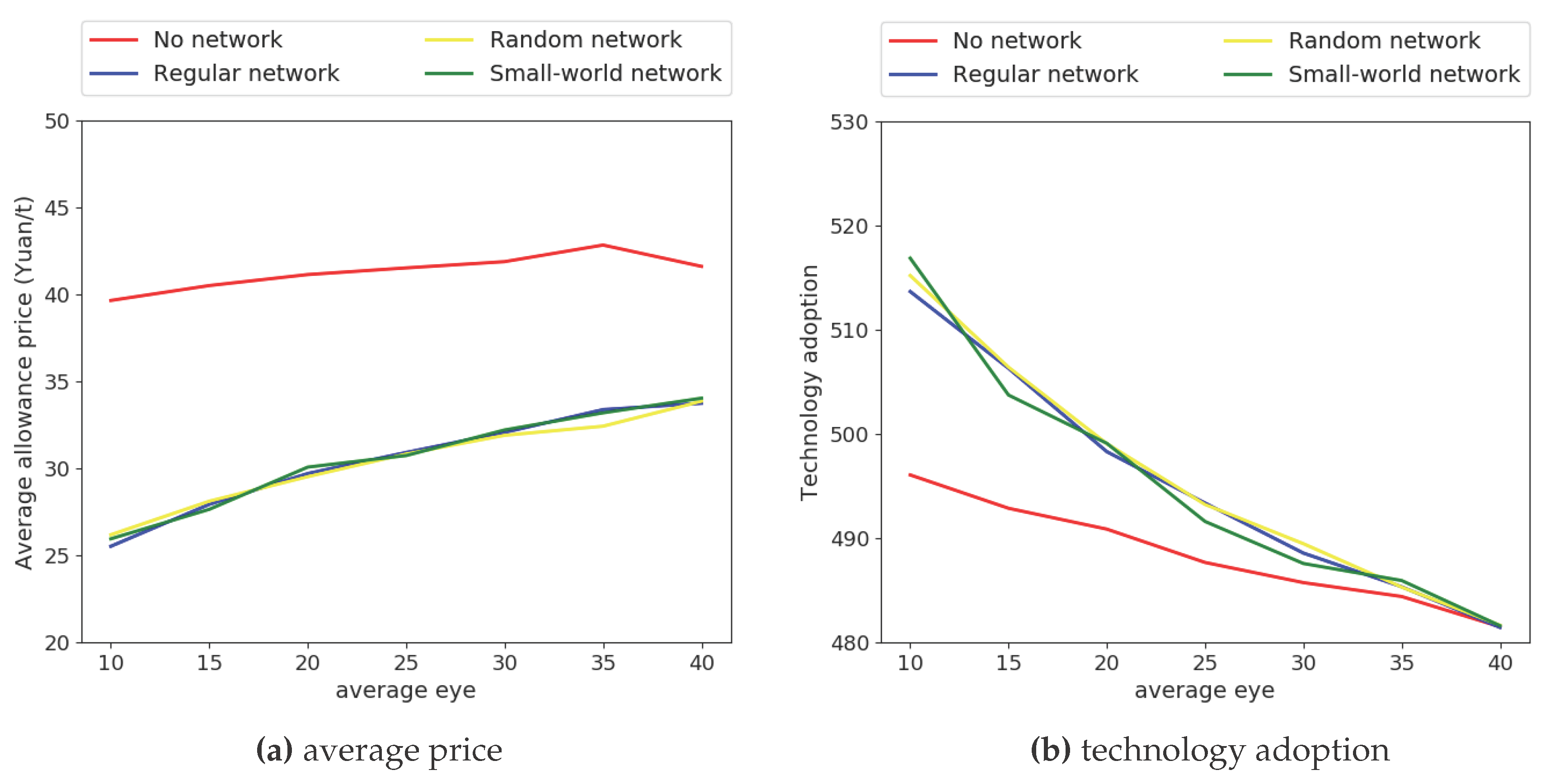
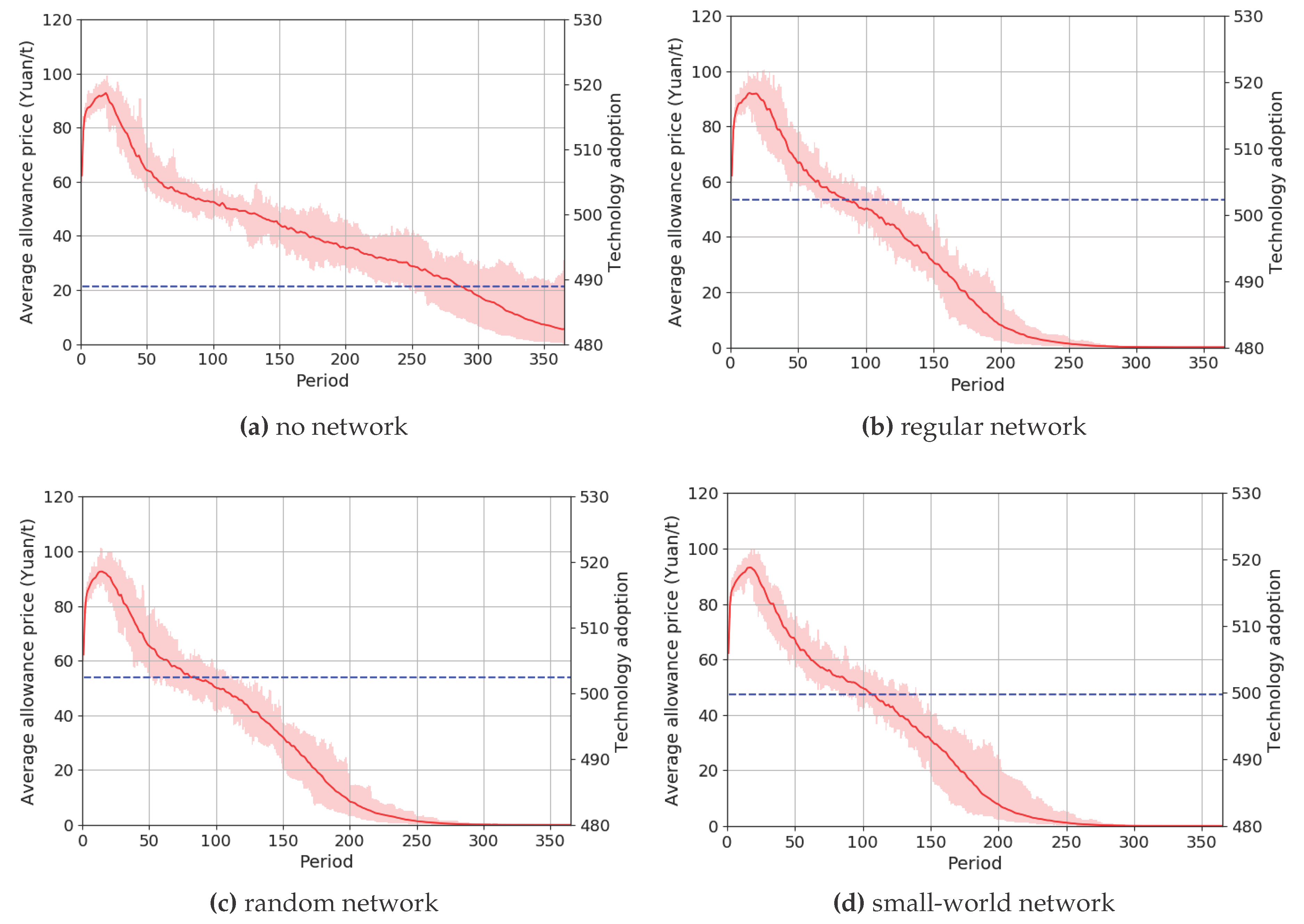
4.1. Allowance Price and Low-Carbon Technology Adoption

As introduced in Section 2.3.1, the agents in the “no network” scenario obtain limited but global information, while the agents in the other three scenarios obtain limited and local information. As a result, when an inefficient adoption of low-carbon technology occurs, it is easier to be observed by more other agents in the “no network” scenario than in the other three scenarios. The agents who observe the inefficient adoptions reduce their forecast of the allowance price immediately, which then leads to a decline of the real allowance price. Thus, more inefficient adoptions of low-carbon technologies can be avoided in the “no network” scenario than in the other three scenarios. The more inefficient adoptions that are avoided, the tighter the allowance supply is, and the higher the average allowance price is. These results are shown in Figure 3.

In Figure 3, the red lines represent the allowance price in the carbon market, and the light red areas represent the variation in 30 simulations. The four horizontal dotted blue lines represent the total technology adoption in each of the scenarios. The “no network” scenario has the least adoptions of low-carbon technologies, which means that the most inefficient adoptions are avoided. Additionally, as a result of more inefficient adoptions of low-carbon technologies, the allowance price falls to zero in the other three scenarios. However, these three scenarios do not exhibit significant differences.

For a similar reason, the increase of $EY{E}_i$ indicates more information for agents to make decisions, which also leads to less inefficient adoptions and a higher average allowance price. The “no network” scenario follows different expansion paths from the other three scenarios when $EY{E}_i$ rises (as shown in Figure 4), while the lines for the other three scenarios entangle with each other, which indicates little difference among them.

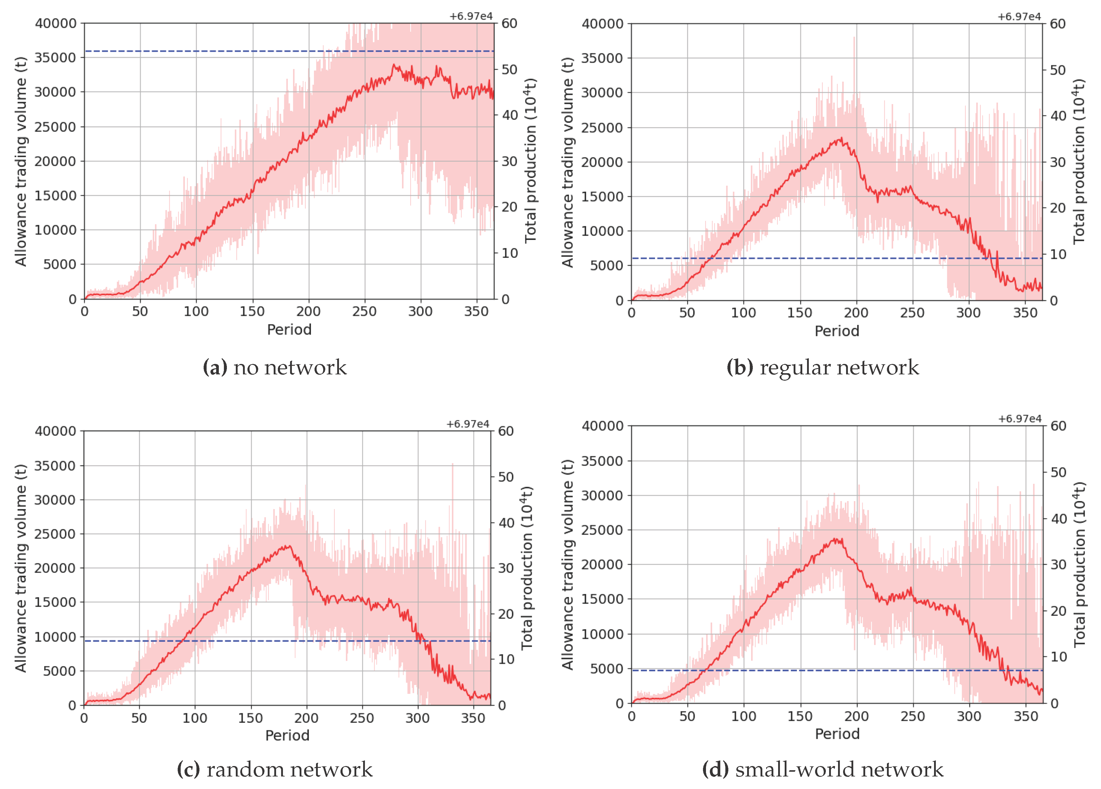
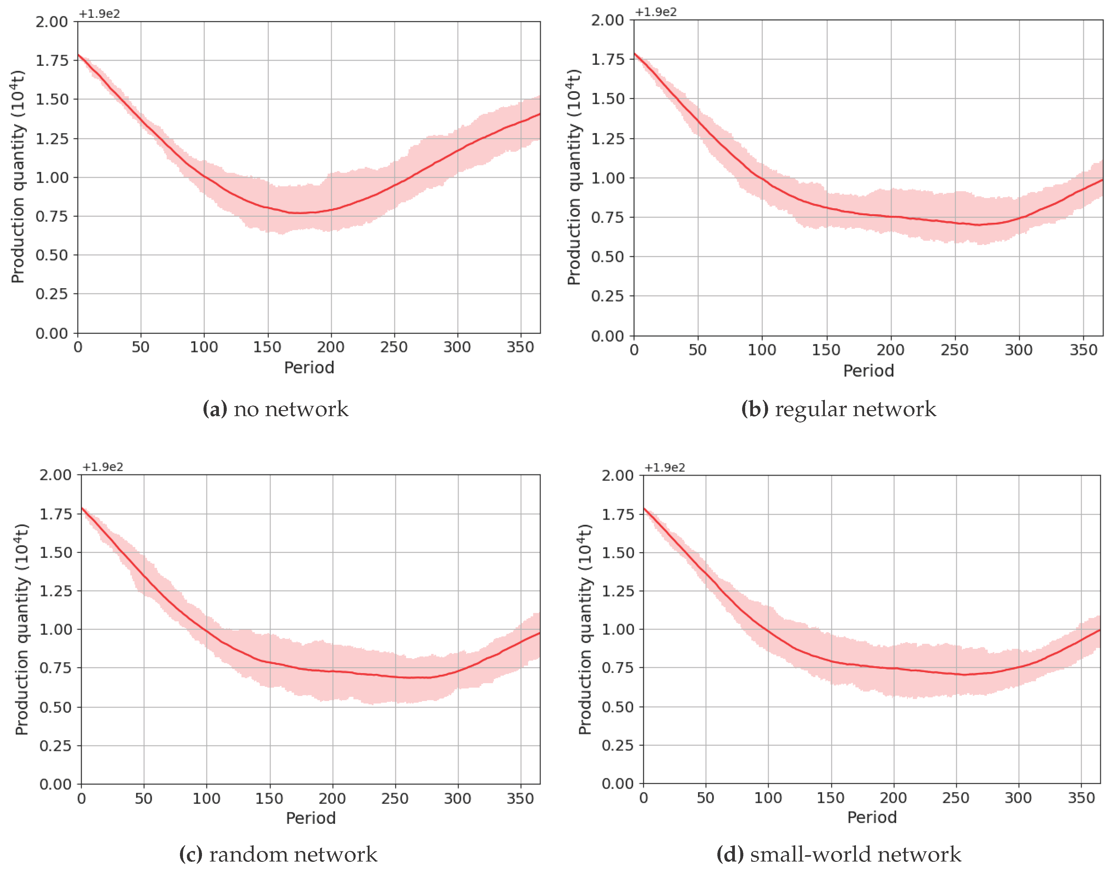
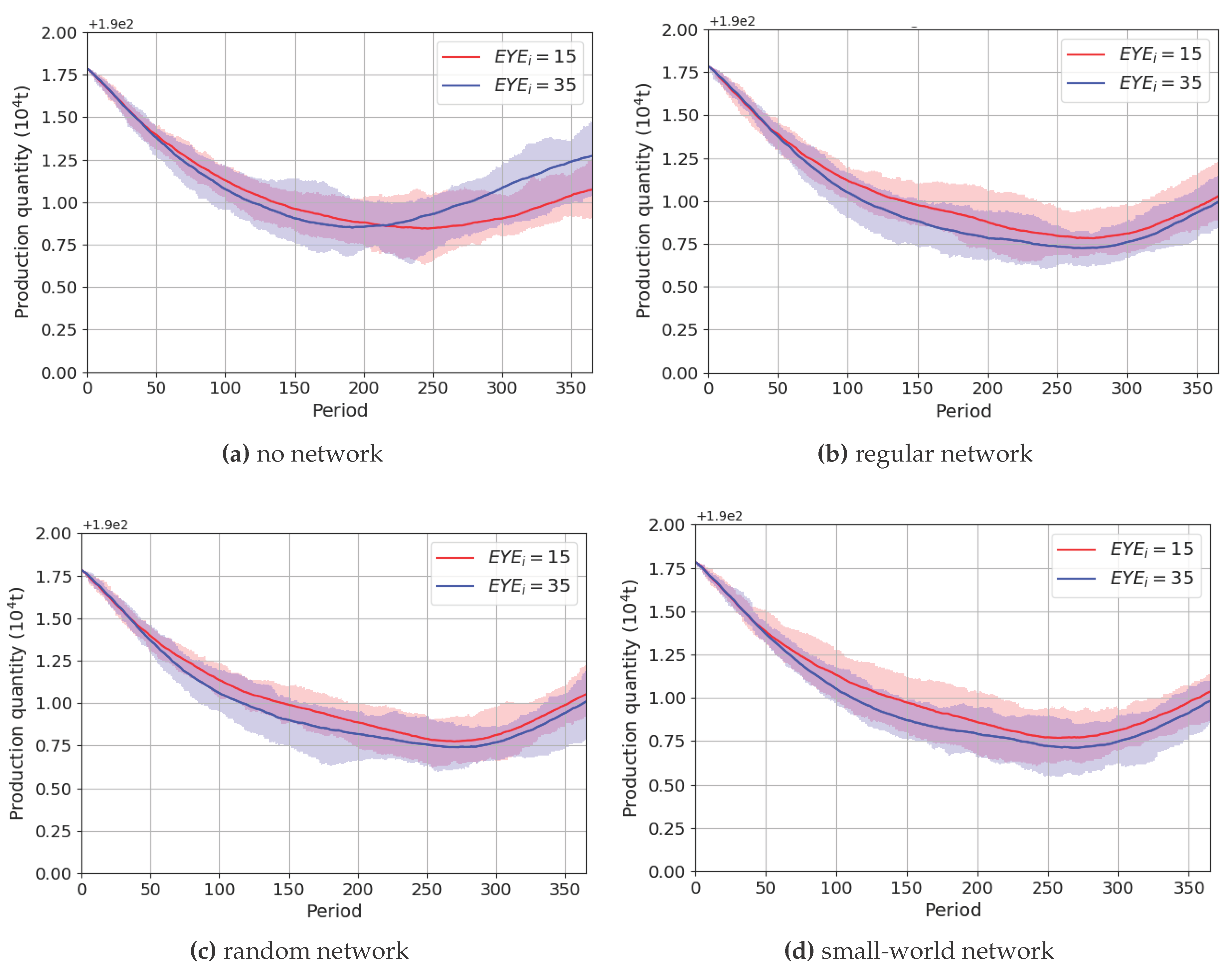
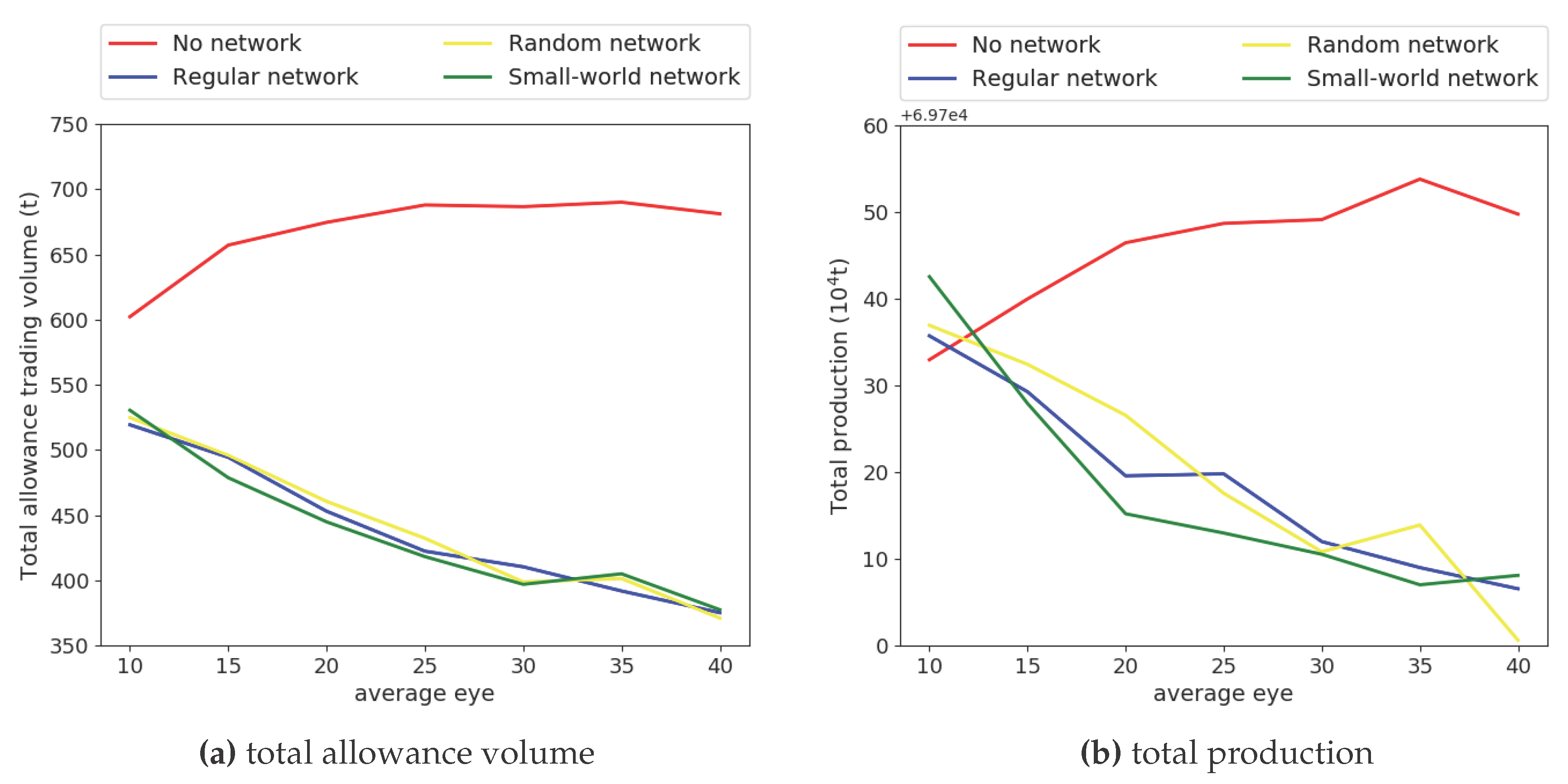
4.2. Allowance Trading Volume and Total Production

Concerning the impact of the network structure on the trading volume of allowance and total production, we also choose the simulation results for four scenarios with the agents’ average $EY{E}_i$ equal to 15 as an example. The relevant results are shown in Figure 5.

In Figure 5, we can see that for the “no network” scenario, firms’ total production— represented by the dotted blue line—is significantly higher than that in the other three scenarios. This is the same for the total trading volume of allowance. As introduced in Section 4.1, this is because firms have limited but global information in the “no network” scenario, and inefficient adoptions of low-carbon technologies are observed by more agents, which leads to a faster decline of both agents’ forecasts and real allowance price compared with in the other three scenarios. Additionally, firms can also adjust their production faster, as shown in Figure 6.

At the same time, the higher total production of agents also leads to a higher trading volume of allowance in the carbon market, as shown in Figure 5. This is because for the firms with high abatement costs by low-carbon technology adoption, the more firms produce, the greater the allowance gap is, and the higher the trading volume of allowance is in the carbon market.

On the other hand, as discussed in Section 4.1, when firms’ average $EY{E}_i$ rises, more inefficient adoptions of low-carbon technologies can be avoided, which also means stronger pressure for firms to reduce their production for abatement. However, as a result of the existence of an observation network, firms’ total production is further higher in the “no network” scenario than in the other three scenarios. This is because although the stronger pressure leads to a sharper reduction of production at the beginning of the abatement phase, the agents in the “no network” scenario can adjust their production faster when they observe the inefficient adoptions of low-carbon technologies, while the agents in the other three scenarios cannot. A comparison between the two examples with average $EY{E}_i$ equal to 15 and 35 is shown in Figure 7.

As a result, the expansion paths of firms’ total trading volume and total production in four scenarios are different: for the “no network” scenario, firms’ total trading volume of allowance increases with average $EY{E}_i$ rising, as well as firms’ total production; while for the other three scenarios, firms’ total trading volume of allowance decreases with average $EY{E}_i$ rising, as well as firms’ total production. This is shown in Figure 8.

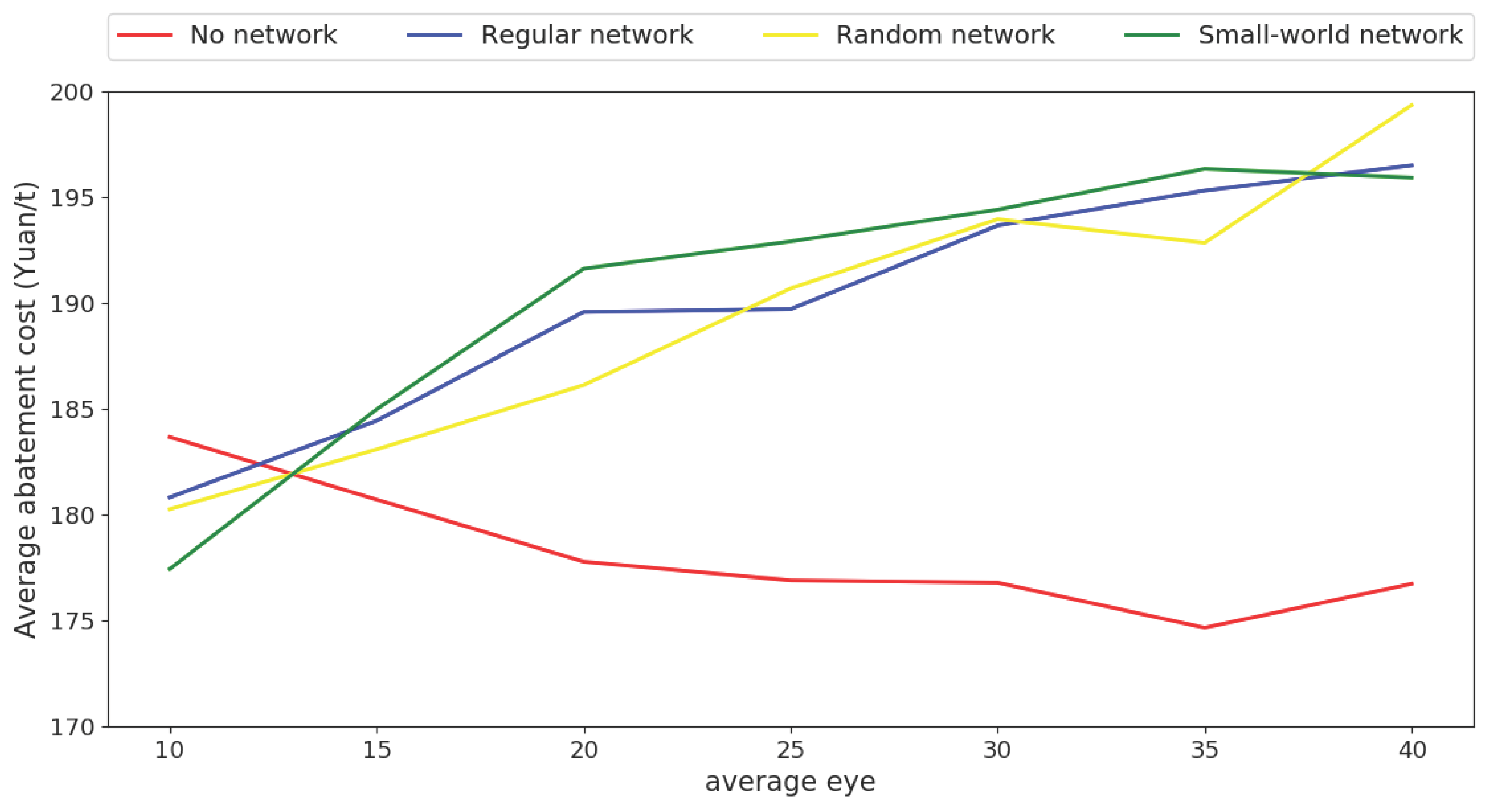
4.3. Efficiency of Carbon Emission Trading Mechanism

In our previous work [10], we found that the efficiency of the carbon emission trading mechanism increases with firms’ rising $EY{E}_i$, which is represented by the decline of the social average abatement cost. However, as discussed in Section 4.2, when the observation network exists, firms’ total production decreases with rising $EY{E}_i$, which means a higher abatement cost of revenue loss in the output market. As a result, the existence of the observation network among firms reverses the trend of the social average abatement cost with firms’ rising $EY{E}_i$, as shown in Figure 9.

5. Conclusions

Based on the agent-based model we established in our previous work [10], we attempt to simulate the impact of the information transmission mechanism on the carbon emission trading scheme. The transmission mechanism is depicted as an observation network among firms. Four scenarios are considered, including no network, regular network, random network, and small-world network.

The simulation results are organized as three parts. First, the impact of different networks on the allowance price and firms’ adoption of low-carbon technologies are analysed. We find that with limited but global information, more inefficient adoptions of low-carbon technologies are avoided in the no network scenario than in the other three scenarios. This leads to lower total adoption of low-carbon technologies, and higher average allowance price. Additionally, when $EY{E}_i$ rises (which indicates more information for firms to make decisions), both firms’ total adoptions and average allowance price rise in all four scenarios. However, the no network scenario follows a different expansion path, and there is no obvious distinction among the other three scenarios. Second, the impact of different networks on the trading volume of allowance and firms’ total production are analysed. We find that the existence of the observation network delays the transmission of information, and also delays firms’ adjustments of production in the output market. This leads to lower total production of firms, as well as a higher revenue loss as the social cost of abatement. Third, following the second result, our model shows that the existence reverses the trend of the social average abatement cost with the increase of firms’ $EY{E}_i$, since the increase of firms’ average $EY{E}_i$ leads to more abatement cost from revenue loss in the output market.

In conclusion, the existence of the observation network shows a significant impact on the carbon emission trading scheme in our model. The most important reason is that when the network exists, it delays the global transmission of fundamental information, which leads to more inefficient adoptions of low-carbon technology and more revenue loss in the output market. In other words, the existence of the observation network reduces the efficiency of the carbon emission trading scheme. In fact, the “no network” scenario we set does not exist in the real world. However, the results and discussions above implicate the necessity of establishing a public mechanism of information disclosure to offset the negative effect of a network that does exist in the real world. According to the results of our simulation, a dynamically updated list of firms’ adoption of low-carbon technologies would help to improve the efficiency of the carbon emission trading scheme.

Finally, several limitations of this model need to be clarified. First, the “firms” in the model only refers to firms with abatement targets in the carbon market, and the financial agents in the real carbon market are not yet included. Second, as a theoretical simulation model, the agent-based model foremost serves as a heuristic device for understanding the evolution of a complex system, scenario analysis, and policy evaluation. In our future work, more work will be done on calibration based on real data and empirical tests of the results of the model. Third, the impact of the carbon emission trading scheme also relies heavily on the allocation mechanism of the allowance. In this paper, the allowance is allocated based on a grandfathering mechanism, so firms’ allocations are not related to their real production. Thus, firms have stronger incentive to reduce their production for abatement, which shares the same view with Fischer and Fox [24]. In our future work, more allocation mechanisms will be analysed.

References

- Sumner, J.; Bird, L.; Dobos, H. Carbon taxes: A review of experience and policy design considerations. Clim. Policy 2011, 11, 922–943. [Google Scholar] [CrossRef]
- Bakam, I.; Matthews, R.B. Emission trading in agriculture: A study of design options using an agent-based approach. Mitig. Adapt. Strateg. Glob. Chang. 2009, 14, 755–776. [Google Scholar] [CrossRef]
- Wu, J.; Fan, Y.; Xia, Y. The Economic Effects of Initial Quota Allocations on Carbon Emissions Trading in China. Energy J. 2016, 37, 129–151. [Google Scholar] [CrossRef]
- Goulder, L.H.; Hafstead, M.A.; Dworsky, M. Impacts of alternative emissions allowance allocation methods under a federal cap-and-trade program. J. Environ. Econ. Manag. 2010, 60, 161–181. [Google Scholar] [CrossRef]
- Cui, L.B.; Fan, Y.; Zhu, L.; Bi, Q.H. How will the emissions trading scheme save cost for achieving China’s 2020 carbon intensity reduction target? Appl. Energy 2014, 136, 1043–1052. [Google Scholar] [CrossRef]
- Damien, D.; Philippe, Q. European Emission Trading Scheme and competitiveness: A case study on the iron and steel industry. Energy Econ. 2008, 30, 2009–2027. [Google Scholar]
- Martin, R.; Muûls, M.; Wagner, U.J. The impact of the European Union Emissions Trading Scheme on regulated firms: What is the evidence after ten years? Rev. Environ. Econ. Policy 2015, 10, 129–148. [Google Scholar] [CrossRef]
- Oestreich, A.M.; Tsiakas, I. Carbon emissions and stock returns: Evidence from the EU Emissions Trading Scheme. J. Bank. Financ. 2015, 58, 294–308. [Google Scholar] [CrossRef]
- Mo, J.L.; Zhu, L.; Fan, Y. The impact of the EU ETS on the corporate value of European electricity corporations. Energy 2012, 45, 3–11. [Google Scholar] [CrossRef]
- Yu, S.; Fan, Y.; Zhu, L. How Do Heterogeneity and Incomplete Information Influence the Carbon Market? An Agent-Based Approach. 2017. Working Paper. Available online: https://www.researchgate.net/project/Agent-based-simulation-for-emission-trading-scheme (accessed on 24 May 2017).
- Zhang, J.; McBurney, P.; Musial, K. Convergence of trading strategies in continuous double auction markets with boundedly-rational networked traders. Rev. Quant. Financ. Account. 2017, 1–52. [Google Scholar] [CrossRef]
- Alfarano, S.; Milaković, M.; Raddant, M. A note on institutional hierarchy and volatility in financial markets. Eur. J. Financ. 2013, 19, 449–465. [Google Scholar] [CrossRef] [Green Version]
- Chapman, M.; Tyson, G.; Atkinson, K.; Luck, M.; McBurney, P. Social networking and information diffusion in automated markets. In Agent-Mediated Electronic Commerce. Designing Trading Strategies and Mechanisms for Electronic Markets; Springer: Berlin, Germany, 2013; pp. 1–15. [Google Scholar]
- Delre, S.A.; Jager, W.; Janssen, M.A. Diffusion dynamics in small-world networks with heterogeneous consumers. Comput. Math. Organ. Theory 2007, 13, 185–202. [Google Scholar] [CrossRef]
- Kocsis, G.; Kun, F. The effect of network topologies on the spreading of technological developments. J. Stat. Mech. Theory Exp. 2008, 2008. [Google Scholar] [CrossRef]
- Janssen, M.A.; Jager, W. Simulating market dynamics: Interactions between consumer psychology and social networks. Artif. Life 2003, 9, 343–356. [Google Scholar] [CrossRef] [PubMed]
- Baker, E.; Clarke, L.; Shittu, E. Technical change and the marginal cost of abatement. Energy Econ. 2008, 30, 2799–2816. [Google Scholar] [CrossRef]
- Bauman, Y.; Lee, M.; Seeley, K. Does technological innovation really reduce marginal abatement costs? Some theory, algebraic evidence, and policy implications. Environ. Resour. Econ. 2008, 40, 507–527. [Google Scholar] [CrossRef]
- Li, Y.; Zhu, L. Cost of energy saving and CO2 emissions reduction in China’s iron and steel sector. Appl. Energy 2014, 130, 603–616. [Google Scholar] [CrossRef]
- Albert, R.; Barabási, A.L. Statistical mechanics of complex networks. Rev. Mod. Phys. 2002, 74, 47–97. [Google Scholar] [CrossRef]
- Watts, D.J.; Strogatz, S.H. Collective dynamics of ‘small-world’ networks. Nature 1998, 393, 440–442. [Google Scholar] [CrossRef] [PubMed]
- Gigerenzer, G. Fast and frugal heuristics: The tools of bounded rationality. In Blackwell Handbook of Judgment and Decision Making; Wiley-Blackwell: Hoboken, NJ, USA, 2004. [Google Scholar]
- Raberto, M.; Cincotti, S.; Focardi, S.M.; Marchesi, M. Agent-based simulation of a financial market. Phys. A Stat. Mech. Appl. 2001, 299, 319–327. [Google Scholar] [CrossRef]
- Fischer, C.; Fox, A.K. Output-based allocation of emissions permits for mitigating tax and trade interactions. Land Econ. 2007, 83, 575–599. [Google Scholar] [CrossRef]
© 2017 by the authors. Licensee MDPI, Basel, Switzerland. This article is an open access article distributed under the terms and conditions of the Creative Commons Attribution (CC BY) license (http://creativecommons.org/licenses/by/4.0/).
Share and Cite
Yu, S.-m.; Zhu, L. Impact of Firms’ Observation Network on the Carbon Market. Energies 2017, 10, 1164. https://doi.org/10.3390/en10081164
Yu S-m, Zhu L. Impact of Firms’ Observation Network on the Carbon Market. Energies. 2017; 10(8):1164. https://doi.org/10.3390/en10081164
Chicago/Turabian StyleYu, Song-min, and Lei Zhu. 2017. "Impact of Firms’ Observation Network on the Carbon Market" Energies 10, no. 8: 1164. https://doi.org/10.3390/en10081164
APA StyleYu, S.-m., & Zhu, L. (2017). Impact of Firms’ Observation Network on the Carbon Market. Energies, 10(8), 1164. https://doi.org/10.3390/en10081164