A Novel Observer for Lithium-Ion Battery State of Charge Estimation in Electric Vehicles Based on a Second-Order Equivalent Circuit Model

Abstract

Accurate state of charge (SOC) estimation can prolong lithium-ion battery life and improve its performance in practice. This paper proposes a new method for SOC estimation. The second-order resistor-capacitor (2RC) equivalent circuit model (ECM) is applied to describe the dynamic behavior of lithium-ion battery on deriving state space equations. A novel method for SOC estimation is then presented. This method does not require any matrix calculation, so the computation cost can be very low, making it more suitable for hardware implementation. The Federal Urban Driving Schedule (FUDS), The New European Driving Cycle (NEDC), and the West Virginia Suburban Driving Schedule (WVUSUB) experiments are carried to evaluate the performance of the proposed method. Experimental results show that the SOC estimation error can converge to 3% error boundary within 30 s when the initial SOC estimation error is 20%, and the proposed method can maintain an estimation error less than 3% with 1% voltage noise and 5% current noise. Further, the proposed method has excellent robustness against parameter disturbance. Also, it has higher estimation accuracy than the extended Kalman filter (EKF), but with decreased hardware requirements and faster convergence rate.

1. Introduction

In recent years, electric vehicles (EVs) have been of increased interest because of the global energy shortage and growing environmental pollution [1]. Many governments are promoting the use of electric vehicles, including battery electric vehicles (BEVs), fuel cell electric vehicles (FCEVs), and hybrid electric vehicles (HEVs). Lithium-ion batteries (LIBs) have found wide application in EVs for their features of high energy/power density, tiny memory effect, and low self-discharge effect [2]. The battery management system (BMS) plays an essential role in improving the battery performance, prolonging battery life, and ensuring its safety [3]. Estimation of the battery state of charge (SOC) is one of the most important functions of BMS. An accurate SOC estimation can prevent the battery from over-charging or over-discharging, improve battery performance, and also help dispel driver anxiety about the potential range of operation [4]. As an indicator of the ratio of the remaining capacity to the rated capacity, SOC is an inner state of a battery, and as such, it cannot be measured directly. To estimate its value, we have to utilize specific mathematical methods incorporating measurable battery parameters, such as current, voltage, and temperature.

In order to get an accurate SOC estimate, many estimation methods have been proposed. Generally, existing estimation methods are non-model-based methods and model-based methods. Some examples of non-model-based methods are the coulomb counting method (Ampere-hour integral method) [5,6], open circuit voltage method [7,8], artificial neural network method (ANN) [9,10,11,12], fuzzy logic method (FL) [13,14,15], and support vector machine method (SVM) [16,17,18]. The coulomb counting method is the most commonly-used method due to its simplicity and low computation cost. However, this method suffers from accumulated errors caused by current measurement noises. Additionally, if the initial SOC estimate is not accurate, the coulomb counting method cannot correct this initial error. The open circuit voltage approach can specify the battery SOC value based on the monotonous relationship between the open circuit voltage and SOC, but it takes several hours for the terminal voltage to reach the equilibrium state, which is obviously impractical in reality. Artificial neural networks, fuzzy logic, and support vector machine methods are intelligent computational algorithms that can theoretically calculate SOC with high precision, but these methods require a significant amount of training data. This training process is time-consuming and almost impossible to accomplish because of the complexity of practical driving conditions. Additionally, these three methods require a powerful microchip to perform the data processing, which will inevitably increase the hardware cost.

Examples of model-based estimation methods include methods based on the Kalman filter (KF) [3,4,17,19,20,21,22,23,24,25,26,27,28], the sliding mode observer (SMO) [29,30,31,32], and the Luenberger observer [33,34,35,36]. The Kalman filter is an optimal recursive estimation method for linear dynamic system. To extend this method to a nonlinear dynamic system, the extended KF (EKF), sigma-point KF (SKF), and unscented KF (UKF) methods for SOC estimation have been proposed. The EKF method uses a first-order Taylor series expansion at each time step to approximate the nonlinear observation function [20,21]. However, a significant problem of EKF is that the estimation errors caused by the local linearization will increase greatly when the battery model has significant nonlinearity. Additionally, the EKF method requires calculation of the Jacobian matrix, which may result in instability of the filter for a strongly nonlinear LIB system. The UKF and SKF methods utilize an unscented transformation to approximate the probability density function of the battery state with a set of sample points. Previous studies have shown that these two methods can effectively improve estimation accuracy, but the computation costs of these two methods are tremendous due to mass matrix calculations during the estimation process [24,26]. Further, all KF-based methods require statistical knowledge of the noises to ensure their estimation accuracy, which we cannot obtain easily in practice. The sliding mode observer (SMO) is an effective SOC estimation method against model uncertainties and external disturbances. However, it is difficult to design optimal parameters such as the switching gains and the uncertainty boundaries for the observer. Additionally, the SMO requires a piecewise linearization method to approximate LIB systems, which will inevitably lead to linearization errors [30]. The Luenberger observer is another commonly used strategy for SOC estimation, but its general applicability is limited, as its parameters are difficult to design [33].

In this paper, a novel method for SOC estimation with a second-order resistor-capacitor (2RC) equivalent circuit model (ECM) is proposed. The validation results show that the proposed method has good performance in terms of estimation accuracy and robustness against measurement noise and parameter uncertainty. This method does not require matrix calculation, so the computation cost is significantly low. Furthermore, the presented method has a higher estimation accuracy and faster convergence rate compared to EKF method. Above all, the proposed method is appropriate for implementation in LIB systems in electric vehicles.

The remainder of this paper is organized as follows. In Section 2, the widely-used 2RC equivalent circuit model is introduced and the state space equations are derived. In Section 3, the design of the proposed method is presented in detail. The experimental configuration and discussion are presented in Section 4. Section 5 concludes the paper.

2. Battery Model

2.1. Battery Equivalent Circuit Model

Selection of the appropriate battery model is required for an accurate model-based estimation method. To accurately simulate the battery characteristics, various battery models have been proposed, such as the thermal model [37], the equivalent circuit model, and the electrochemical model [38]. Of these, equivalent circuit models (ECMs) are commonly-used to simulate the dynamic behavior of the battery, including the voltage response to different current condition. ECMs include the partnership for a new generation of vehicle (PNGV) model, the Rint model, the Thevenin model, and the second-order resistor-capacitor (2RC) model [39]. These modes consist of basic circuit components such as voltage sources, resistors, and capacitors. Generally speaking, adding resistor-capacitor (RC) series will improve model accuracy and increase the structural complexity of the model [40]. In this paper, an equivalent circuit model with two RC networks was selected and it consists of a resistor R_o, two RC networks, and a voltage source U_oc (SOC). The schematic diagram of the model is shown in Figure 1. In the model, R_o denotes the ohmic resistance of the lithium-battery. R₁ and C₁ denote the electrochemical polarization resistance and capacitance, respectively. R₂ and C₂ denote the concentration polarization resistance and capacitance, respectively. I_t represents the current flowing through the voltage source. The output voltage of the voltage source is denoted by U_oc, which has a monotonous relationship with the SOC of the battery.

Here, U₁, U₂ and SOC are taken as state variables and U_L is the observation variable. The state equations of the equivalent circuit model can be derived as:

$${\dot{U}}_1=-\frac{1}{R_1{C}_1}{U}_1+\frac{1}{C_1}{I}_t$$

(1)

$${\dot{U}}_2=-\frac{1}{R_2{C}_2}{U}_2+\frac{1}{C_2}{I}_t$$

(2)

$$\dot{\mathrm{S}}\mathrm{OC}=-\frac{1}{Q_n}{I}_t$$

(3)

where ${\dot{U}}_1$, ${\dot{U}}_2$, $\dot{\mathrm{S}}\mathrm{OC}$ represent the derivative of $U_1$, $U_2$, and $\mathrm{SOC}$, respectively. Q_n is the discharge capacity of the battery. The observation equation can be derived as:

$$U_L=U_{OC}(\mathrm{SOC})-U_1-U_2-I_t{R}_o$$

(4)

2.2. Parameter Identification

Before the ECM described above can be used for SOC estimation, the values of parameters (U_oc (SOC), R_o, R₁, C₁, R₂, and C₂) need to be identified. U_oc (SOC) describes the relationship between the output voltage of the lithium battery and SOC, which can be obtained by fitting experimental data. The experiment is implemented based on a Samsung ICR18650-22P lithium-ion battery under a constant temperature of 25 °C. More details about the battery are listed in Section 4.1. The test procedure is as follows: (1) fully charge the battery with constant current and constant voltage (CC-CV) method and then leave the battery in the open circuit condition for 30 min; (2) discharge the battery at a rate of 1 C until reaching the cut-off voltage at 2.75 V and then record the discharge capacity Q_n; (3) fully charge the battery with CC-CV method and then leave the battery in the open circuit condition for 2 h; (4) record the voltage of the battery as the open circuit voltage of the battery with 100% SOC; (5) discharge the battery to 95% SOC at a rate of 1 C; (6) leave the battery in the open circuit condition for 2 h, and record the voltage as the open circuit voltage of the battery with 95% SOC; and then (7) repeat steps (5) and (6) to separately measure the open circuit voltage of the battery with SOC of 90%, 80%, 70%, 60%, 50%, 40%, 30%, 20%, 15%, 10%, 5%, and 0%.

Table 1. Measured open circuit voltage (OCV) at different SOCs for 25 °C.

SOC(%)	100	95	90	80	70	60	50	40	30	20	15	10	5	0
OCV (V)	4.18	4.12	4.08	4.02	3.94	3.88	3.78	3.68	3.63	3.6	3.58	3.53	3.48	3.45

lists the measured voltage data. A sixth-order polynomial is then utilized to fit the experimental data. Equation (5) is the fitting result and the relationship between U_oc and SOC can been denoted as g(SOC). The measured data and the fitted curve are shown in Figure 2, in which the blue plus signs represent the measured data and the red solid line is the fitted curve. As shown, the sixth-order polynomial can approximate well the voltage property of the lithium-ion battery. Further, strong nonlinearity of the LIB can be observed from the data presented in Figure 2.

$$\begin{array}{l}{U}_{oc}=12.2581\times {\mathrm{SOC}}^6-28.8126\times {\mathrm{SOC}}^5+20.7236\times {\mathrm{SOC}}^4-2.6045\times {\mathrm{SOC}}^3\\ -1.9103\times {\mathrm{SOC}}^2+1.0889\times \mathrm{SOC}+3.4444\end{array}$$

(5)

The other parameters (R_o, R₁, C₁, R₂, and C₂) can be determined from measured voltage data from a pulse-current discharging process using an exponential-function fitting method [41]. The pulse-current profile consists of a 330-s discharging period with constant current of 2.2 A (about 1 C) and a 3600-s rest period. Here, the transient response of terminal voltage data at 60% SOC was utilized to calculate these parameters. Measured terminal voltage response is shown in Figure 3. According to Figure 3, the terminal voltage during the relaxation period can be fitted with the exponential function in the form of Equation (6).

$$U_L=k_0-k_1\exp (-{\lambda }_{1}t)-k_2\exp (-{\lambda }_{2}t)$$

(6)

At the same time, based on the ECM proposed in Section 2.1, the terminal voltage in relaxation period can be expressed as Equation (7):

$$U_L=U_{oc}-R_o{I}_t-R_1{I}_t\exp (-t/R_1{C}_1)-R_2{I}_t\exp (-t/R_2{C}_2)$$

(7)

Comparing Equation (6) with Equation (7), then we could obtain the values of R₁, C₁, R₂, C₂ as:

$$R_1=k_1/I_t,R_2=k_2/I_t,C_1=1/({\lambda }_1{R}_1),C_2=1/({\lambda }_2{R}_2)$$

R_o can derive from the instant voltage increase when the discharging current stops, since the ohmic resistance can be taken as the only factor causing the voltage increase at first. The value of R_o can be obtained by Equation (8) in which ΔU is the step-variation of terminal voltage at the moment of discharging process stops. Here, ΔU is chosen as voltage increment of the first second in relaxation period. The values of the identified parameters are listed in

Table 2. Parameters of the 2RC ECM (equivalent circuit model).

Parameters	Ro (Ω)	R1 (Ω)	R2 (Ω)	C1 (F)	C2 (F)
Values	0.03417	0.02221	0.01902	1498.26	65453.28

. In practical application, the values of these parameters change dynamically due to various factors such as depth of discharge, ambient temperature, age effect, etc. Also, there are a number of studies about online parameter identification methods [42,43,44,45], which can be used to identify model parameters in real time. However, this is beyond the scope of this paper.

$$R_o=\Delta U/I_t$$

(8)

2.3. Model Validation Test

In order to verify the established 2RC ECM, the Urban Dynamometer Driving Schedule (UDDS) test is implemented. The complete current profile is shown in Figure 4a, and b is a magnified portion of the data in Figure 4a. Figure 4c depicts the comparison between the measured voltage and the model output voltage, and Figure 4d shows the model output voltage error for Figure 4c. The average voltage error between the measured voltage and the model output is 0.007 V, with a maximum error of 0.025 V. From Figure 4, we can see that the 2RC ECM can track the dynamic voltage properties of the lithium-ion battery precisely.

3. Design of the Novel Observer

Observers are widely-used in state estimation problems to eliminate state estimation error using deviation feedback. For SOC of a LIB, most existing observers utilize the difference between the estimation output voltage and the measured voltage multiplied by coefficients to correct all of the estimated states [46,47]. There are several disadvantages of these observers. First, the optimal gain coefficients are hard to determine. Second, some observers utilize a linearization method to approximate the nonlinear relationship between the open circuit voltage and SOC, which inevitably causes linearization error [29].

According to Equations (1)–(3), the three state variables change independently. The estimation error is mainly caused by an inaccurate SOC estimated value. To improve estimation accuracy and simplify the structural complexity of the observer, we designed a new observer as follows:

$${\dot{\widehat{U}}}_1=-\frac{1}{R_1{C}_1}{\widehat{U}}_1+\frac{1}{C_1}{I}_t$$

(9)

$${\dot{\widehat{U}}}_2=-\frac{1}{R_2{C}_2}{\widehat{U}}_2+\frac{1}{C_2}{I}_t$$

(10)

$$\dot{\widehat{\mathrm{S}}}\mathrm{OC}=-\frac{I_t}{Q_n}+c(U_L-{\widehat{U}}_L)$$

(11)

The corresponding observation equation is:

$${\widehat{U}}_L=g(\widehat{\mathrm{S}}\mathrm{OC})-{\widehat{U}}_1-{\widehat{U}}_2-I_t{R}_o$$

(12)

In which ${\widehat{U}}_1$, ${\widehat{U}}_2$, and $\widehat{\mathrm{S}}\mathrm{OC}$ are the estimations of the state variables $U_1$, $U_2$, and $\mathrm{SOC}$, respectively. ${\widehat{U}}_L$ is the estimation of the observation variable $U_L$, and c is the observer gain. By assuming that ${\tilde{U}}_1=U_1-{\widehat{U}}_1$, ${\tilde{U}}_2=U_2-{\widehat{U}}_2$, $\tilde{\mathrm{S}}\mathrm{OC}=\mathrm{SOC}-\widehat{\mathrm{S}}\mathrm{OC}$, the dynamic equation for errors could be derived as:

$${\dot{\tilde{U}}}_1=-\frac{1}{R_1{C}_1}{\tilde{U}}_1$$

(13)

$${\dot{\tilde{U}}}_2=-\frac{1}{R_2{C}_2}{\tilde{U}}_2$$

(14)

$$\dot{\tilde{\mathrm{S}}}\mathrm{OC}=-c(U_L-{\widehat{U}}_L)$$

(15)

Generally, the Lyapunov stability theory is utilized to prove the stability of observers. Here, considering the specific characteristic of the proposed observer, we do not require Lyapunov stability theory because as long as we have some knowledge of the solution for ordinary differential equations, we can prove that ${\tilde{U}}_1$,${\tilde{U}}_2$, $\tilde{\mathrm{S}}\mathrm{OC}$ asymptotically converge to zero. For Equation (13), this is solved as:

$${\tilde{U}}_1(t)={\tilde{U}}_1(0)e^{-\frac{t}{R_1{C}_1}}$$

(16)

Since $R_1{C}_1>0$, we have $\underset{t\to \infty }{\lim }{\tilde{U}}_1(t)=0$ despite $U_1(0)$.

Also, for Equation (14), it has the solution as

$${\tilde{U}}_2(t)={\tilde{U}}_2(0)e^{-\frac{t}{R_2{C}_2}}$$

(17)

Since $R_2{C}_2>0$, we have $\underset{t\to \infty }{\lim }{\tilde{U}}_2(t)=0$ despite $U_2(0)$.

Substitution of Equations (4) and (12) into Equation (15) allows simplification as Equation (18) according to the Lagrange Mean Value Theorem.

$$\dot{\tilde{\mathrm{S}}}\mathrm{OC}=-c((g(\mathrm{SOC})-U_1-U_2-I_t{R}_o)-(g(\widehat{\mathrm{S}}\mathrm{OC})-{\widehat{U}}_1-{\widehat{U}}_2-I_t{R}_o))=-c(\dot{g}(\mathsf{\eta })\tilde{\mathrm{S}}\mathrm{OC}-{\tilde{U}}_1-{\tilde{U}}_2)$$

(18)

Where $\mathsf{\eta }$ is between $\mathrm{SOC}$ and $\widehat{\mathrm{S}}\mathrm{OC}$. Considering that $\underset{t\to \infty }{\lim }{\tilde{U}}_1(t)=0$ and $\underset{t\to \infty }{\lim }{\tilde{U}}_2(t)=0$, then Equation (18) could be simplified as:

$$\dot{\tilde{\mathrm{S}}}\mathrm{OC}\approx -c\dot{g}(\mathsf{\eta })\tilde{\mathrm{S}}\mathrm{OC}$$

(19)

Since the expression $g(\mathrm{SOC})$ has been determined in Equation (5), we can easily calculate the $\dot{g}(\mathrm{SOC})$. In this case, 0 ≤ η ≤ 1, 0.4 ≤ $\dot{g}(\mathrm{SOC})$ According to differential equation theory, as long as c > 0, we have $\underset{t\to \infty }{\lim }\tilde{\mathrm{S}}\mathrm{OC}(t)=0$ despite $\tilde{\mathrm{S}}\mathrm{OC}(0)$. Thus, we can prove that the proposed observer is stable.

When using this observer for SOC estimation, the value of c cannot be selected arbitrarily. If the value of c is too small, the convergence rate is slow. In contrast, the estimation process may diverge from the true SOC when the value of c is too large. Here, we design an adaptive law in the form of Equation (20) that allows the value of c change dynamically according to the deviation between the measured voltage and model output voltage. In Equation (20), c₀, α, β are parameters designed to adjust the adaptive property of c. Among them, c₀ determines the convergence rate of the proposed observer at first “inaccurate” stage. α and β are used to adjust observer gain when the SOC estimation reach “accurate” stage. There are several requirements need to be met when trying to determine the value of c₀, α, and β: (1) the value of c should be bigger than zero to ensure the stability of the proposed observer; (2) when the voltage estimation error is large, which usually means that SOC estimation error is large, the value of c should be big enough to ensure a fast convergence rate; (3) when the voltage estimation error is small, the value of c should be small enough to avoid SOC estimation “jitter” effect. Considering the aforementioned requirements and characteristics of exponential function in Equation (20), c₀, α, and β were selected as 0.1, −0.09, −10, respectively. Figure 5 shows the relationship between c and $|U_L-{\widehat{U}}_L|$. Figure 6 shows the schematic diagram of the proposed observer.

$$c=c_0+\alpha \exp (\beta |U_L-{\widehat{U}}_L|)$$

(20)

4. Experiments and Discussion

4.1 The Test Bench

The schematic diagram of the test bench is shown in Figure 7. It consists of battery testing equipment (Arbin BT-5HC, Arbin Instruments, College Station, TX, USA), temperature chamber (Sanwood SC-80-CC-2, Sanwood, Dongguan, China), a lithium-ion battery (ICR18650-22P, Samsung SDI, Shenzhen, China), and a personal computer (PC) with Arbin’ Mits Pro Software (v7.0), used for battery charging/discharging control and recording data. Detials about the tested battery include: nominal capacity 2200 mAh, nominal voltage 3.6 V, charging end voltage 4.2 V, discharging end voltage 2.75 V, and maximum continuous discharging current 10 A. The voltage and current measurement errors of the battery testing equipment are less than 0.02% full scale range (FSR). The study was implemented under controlled temperatures. Except Section 4.5, all the other experiments mentioned in this paper were implemented under 25 °C. During battery test operation, a one second measurement sampling time for voltage and current was used.

4.2. Federal Urban Driving Schedule (FUDS) Test

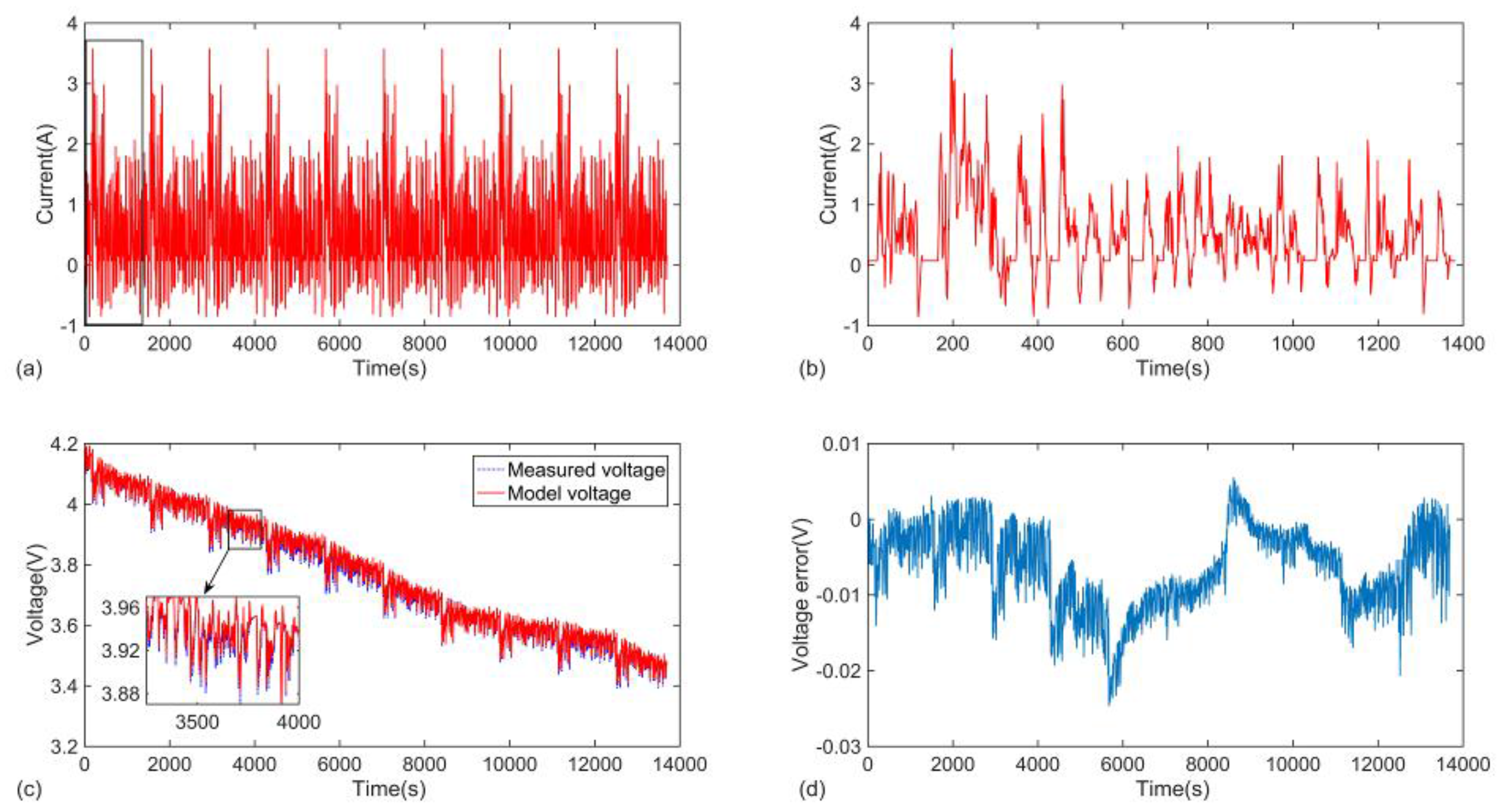
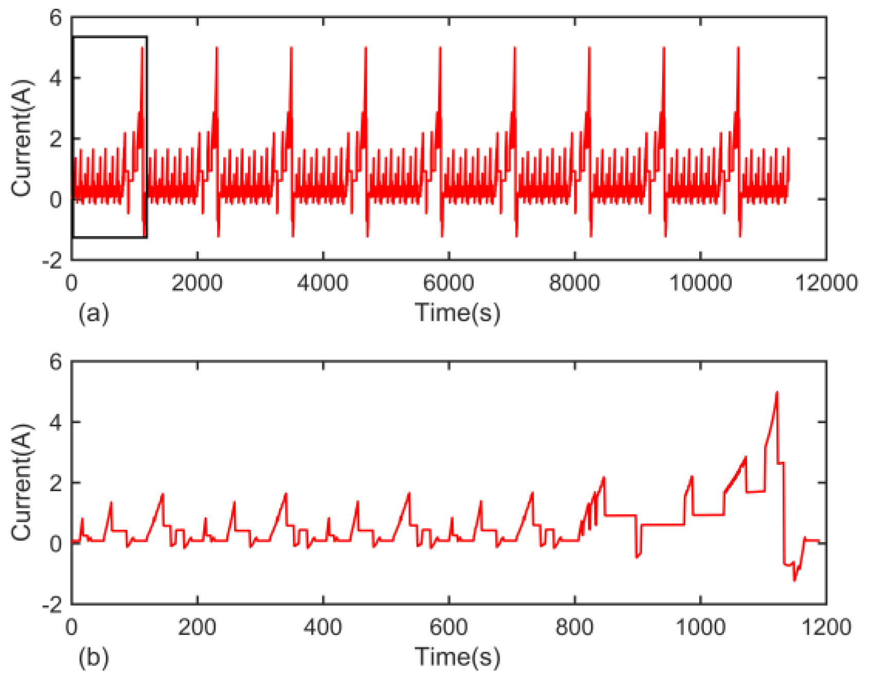
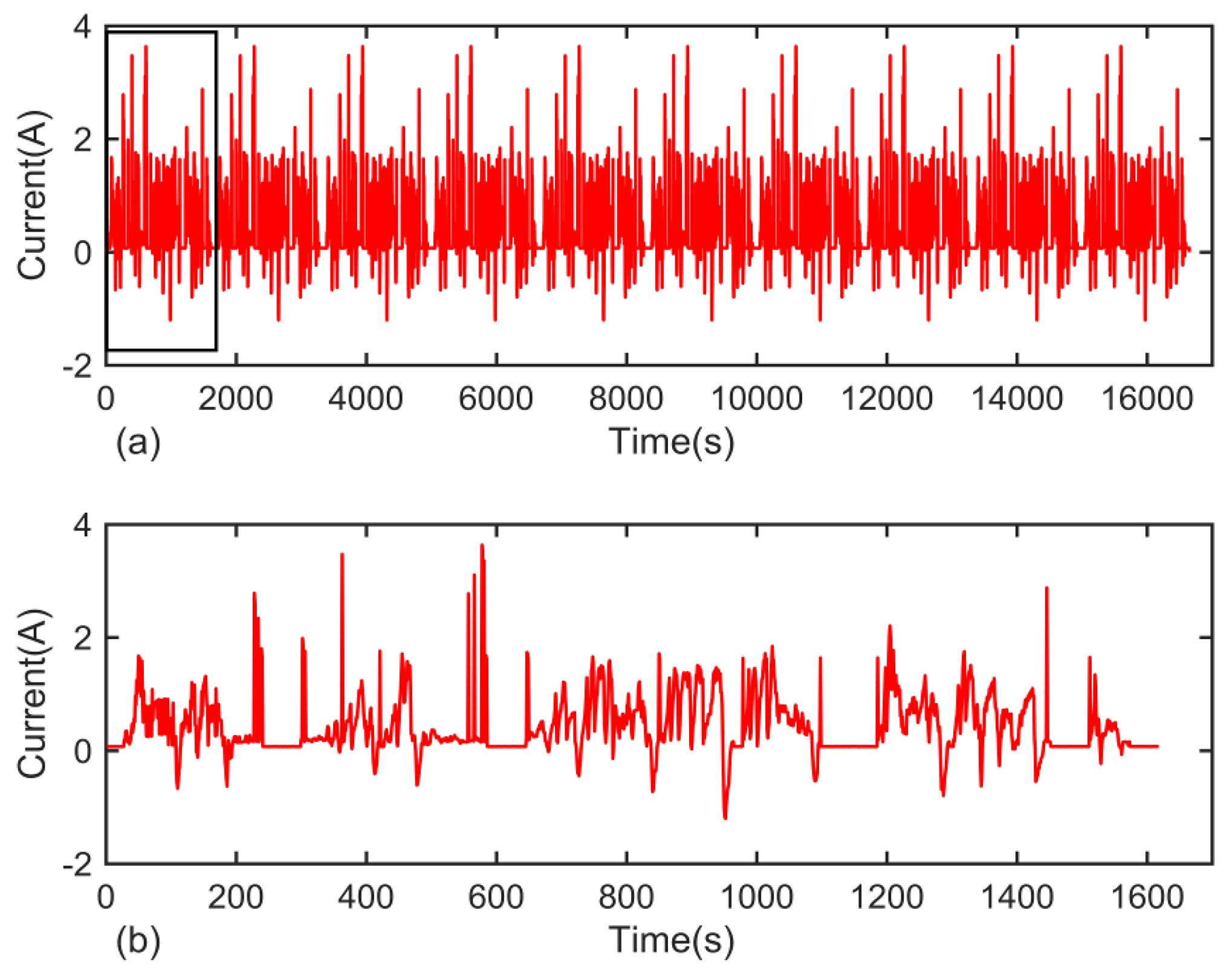
To evaluate the performance of the proposed SOC estimation algorithm, the Federal Urban Driving Schedule (FUDS) test was implemented to simulate a typical loading condition. The current profile of the FUDS test is showed in Figure 8, in which the positive values represent the discharging process and the negative values represent the charging process. Figure 8a displays the complete current vs. 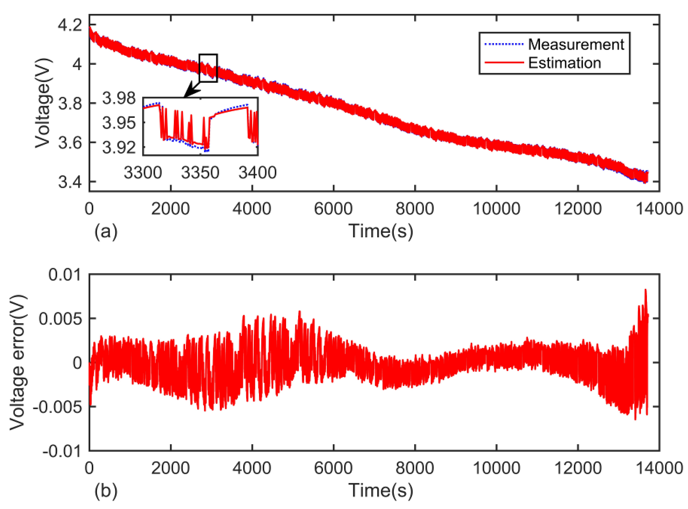time during the FUDS condition, and Figure 8b displays a zoomed part of Figure 8a, as indicated. The measured voltage and estimated voltage under the FUDS test are shown in Figure 9a, and the corresponding voltage estimation error is shown in Figure 9b. In Figure 9a, the blue dotted line is the reference voltage measured with a high precision sensor, and the red solid line is the voltage estimated with the proposed observer. It is obvious that the measured voltage fluctuates greatly due to the sharply changing current, but the estimated voltage can track the measured voltage accurately with a maximum voltage error less than 0.01 V.

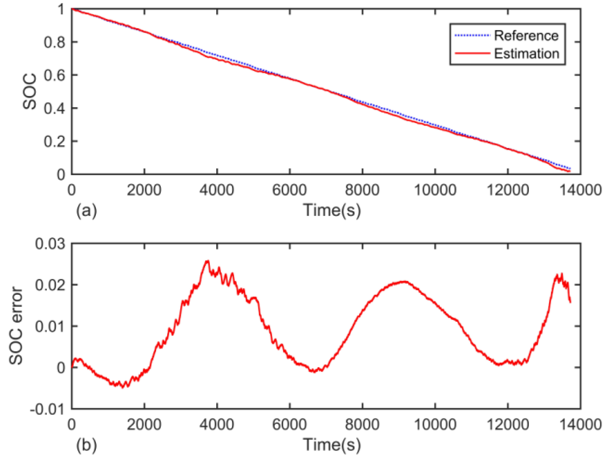
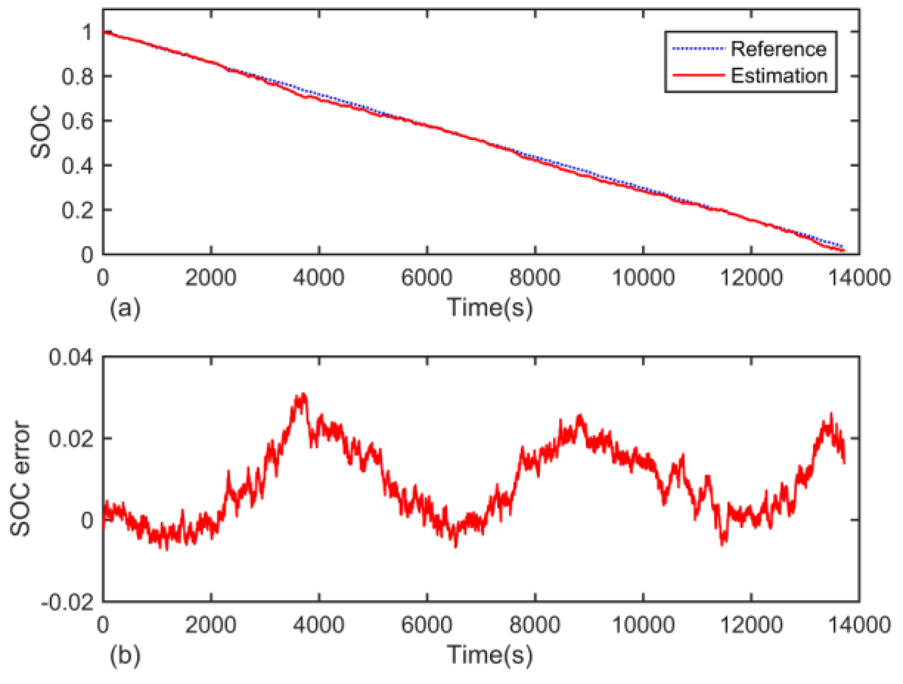
The SOC estimation results under the FUDS test are shown in Figure 10a. The blue dotted line is the reference SOC obtained by the coulomb counting method with high precision sensors, and the red solid line is the estimated SOC. Figure 10b shows the SOC estimation error. From Figure 10b, we can see that the maximum error is lower than 3%. This indicates that the proposed method has good performance for voltage and SOC estimation accuracy.

4.3 Convergence Rate Test

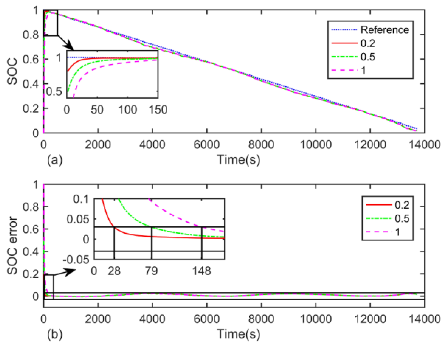
As presented in Section 4.2, we assume that the initial SOC value is equal to the true SOC value. However, in practice, the initial SOC value may not be accurate due to various factors, such as the self-discharge phenomenon and the capacity recovery effect. A good SOC estimation method should compensate for the effect caused by the initial SOC estimation error and converge to the true SOC value within a limited time. In this section, different initial SOC values were set to verify the performance of the proposed observer against the initial SOC estimation error. To be more specific, the initial SOC values are set as 0, 0.5, or 0.8 when the true SOC value is 1. The SOC estimation results are shown in Figure 11a, in which the blue dotted line is the reference SOC. The red solid line, green dash-dotted line, and magenta dash line are the estimated SOCs with an initial SOC estimation error of 0.2, 0.5, and 1, corresponding to the initial SOC values of 0.8, 0.5, and 0, respectively. Figure 11b displays the SOC estimation error. From Figure 11, it is notable that the SOC error decreases dramatically in the first few seconds. The proposed observer has considerable convergence rate.

4.4. Robustness Against Current and Voltage Noises

In Section 4.2 and Section 4.3, we assume that the current and voltage values are accurate, which could be guaranteed under laboratory conditions. However, in practice, the measured current and voltage values are inevitably mixed with noises due to various factors, such as errors in sensor precision, or electromagnetic interference (EMI). Thus, it is important to evaluate the robustness of the proposed observer against measurement noise.

To evaluate the robustness of the proposed observer against the current noise, a sequence of stochastic normal distributed noises was attached to the measured current shown in Figure 8. The mean value of the noise is zero and its standard deviation can be obtained from Equation (21).

$$\sigma =\omega I_{\max }/3$$

(21)

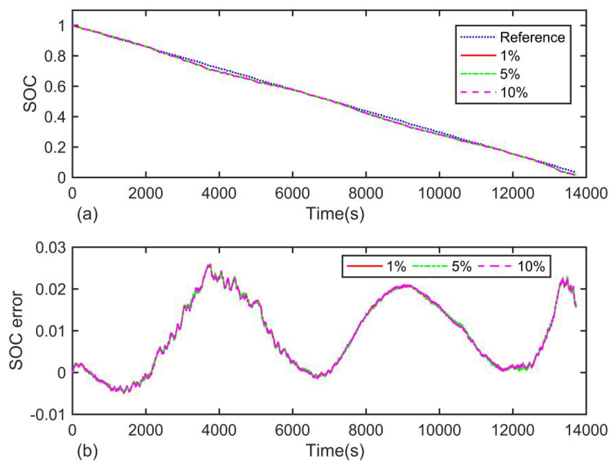
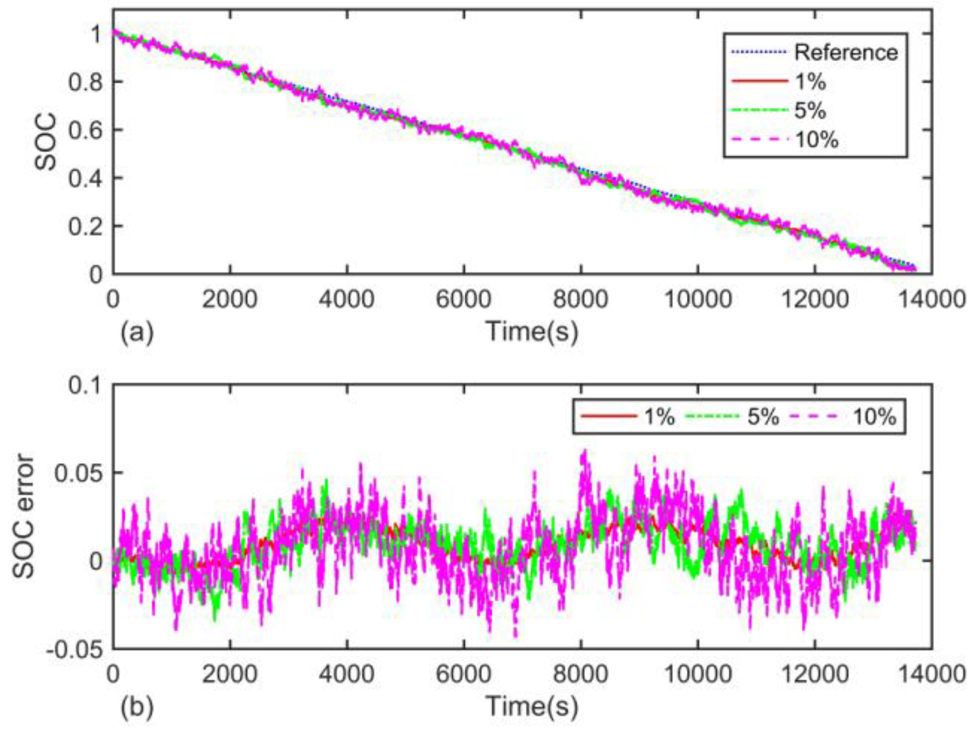
In Equation (21), σ is the standard deviation, ω is a scale factor, and I_max represents the maximum current value from the data shown in Figure 8. We studied the conditions of ω = 1%, 5%, and 10%. The SOC estimation results are shown in Figure 12a,b displays the corresponding SOC estimation error.

In Figure 12a, the blue dotted line is the reference SOC. The red solid line, green dash-dotted line, and magenta dash line represent the estimated SOC with 1%, 5%, and 10% current noises, respectively. To quantitatively study the robustness of the proposed observer, the mean absolute error (MAE) and maximum error were calculated, as listed in

Table 3. SOC estimation errors with different current noises under the FUDS test.

Current Noise Factor (ω)	1%	5%	10%
MAE	0.97%	0.97%	0.98%
Maximum error	2.58%	2.59%	2.59%

. From Figure 12 and Table 3, we can see that although the SOC error fluctuates more intensely as the current noise increases, the mean absolute error and the maximum error of SOC estimation change only slightly.

In practical application, due to factors such as changing temperature and poor calibration, the current sensors may suffer from drift error. To further verify the robustness of the proposed observer against current noises, another test was conducted. Here, a combination of 5% I_max current offset noise and Gaussian noise in the form of Equation (21) with ω = 5% was attached to the current profile, shown in Figure 8. 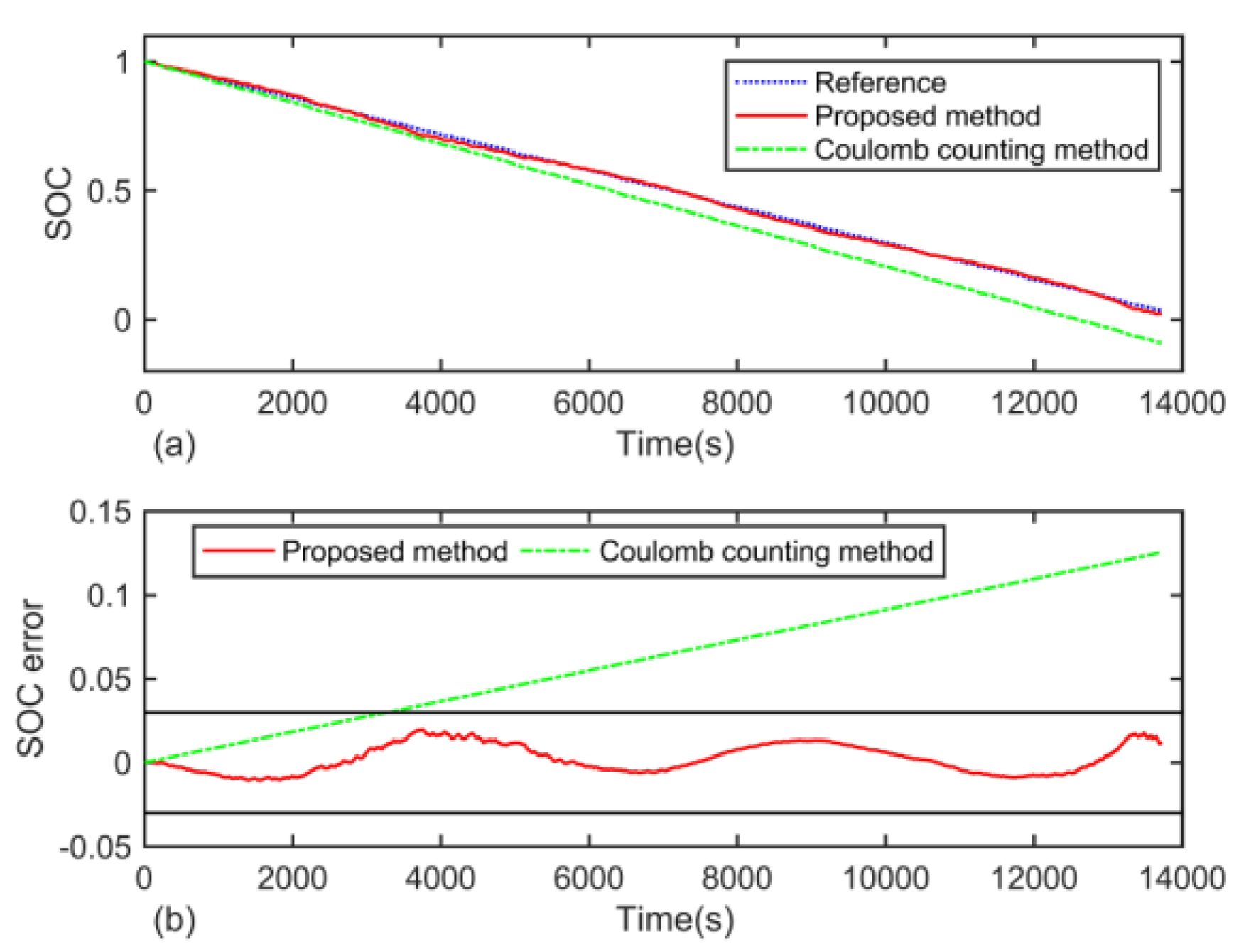Figure 13a shows the SOC estimation result for comparison with the coulomb counting method and Figure 13b displays the corresponding SOC estimation error.

In Figure 13a, the blue dotted line is the reference SOC. The red solid line and green dash-dotted line are the ones calculated by the proposed observer and coulomb counting methods, respectively. In Figure 13b, the black solid lines indicate the 3% SOC error boundary. From Figure 13, we can see that when the current data is inaccurate, the coulomb counting method suffers accumulated error, which is consistent with available literature. In contrast, the proposed observer can well compensate for the current noise and maintain high estimation accuracy.

Similarly, the robustness of the proposed observer against voltage noise was studied. In this test, the voltage noise was assumed to obey a stochastic normal distribution. The mean of the voltage noise is zero, and the standard deviation can be obtained by Equation (22).

$$\sigma =\omega U_{\max }/3$$

(22)

Where σ is the standard deviation, ω is a scale factor, and U_max denotes the maximum measured voltage in the FUDS test described in Section 4.2. In this paper, the conditions of ω = 1%, 5%, and 10% were studied. The SOC estimation results shown in Figure 14a,b display the corresponding SOC estimation error. In Figure 14a, the blue dotted line represents the reference SOC. The red solid line, green dash-dotted line, and magenta dash line are the SOC estimation results for 1%, 5%, 10% voltage noise, respectively.

Table 4. SOC estimation errors with different voltage noises under the FUDS test.

Voltage Noise Factor (ω)	1%	5%	10%
MAE	1.00%	1.23%	1.59%
Maximum error	2.76%	4.61%	6.40%

lists the estimation errors.

As shown in Figure 14a, the estimated SOC fluctuated greatly with the increase of voltage noise. This result is confirmed by Figure 14b, as well as Table 4. Considering that the proposed observer relies on the difference between the measured voltage and the estimated voltage to correct the estimated SOC value, it is of vital importance to obtain accurate voltage values.

Finally, to verify the performance of the proposed observer for an environment containing both current and voltage noise, another test was conducted. In this test, 5% current noise and 1% voltage noise were added to the current profile and voltage profile described in Section 4.2. The estimation results are shown in Figure 15a,b displays the SOC estimation error. In Figure 15a, the blue dotted line is the reference SOC, and the red solid line represents the estimated SOC calculated by the proposed observer in the presence of both current and voltage noises.

Table 5. SOC estimation error in the presence of both current and voltage noises.

Method	The Proposed Observer
MAE	0.98%
Maximum error	3.10%

lists the estimation error.

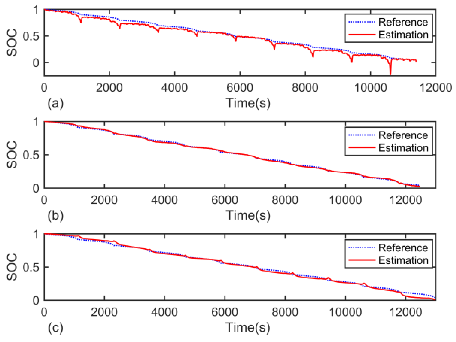
4.5. Robustness Against Parameter Disturbance

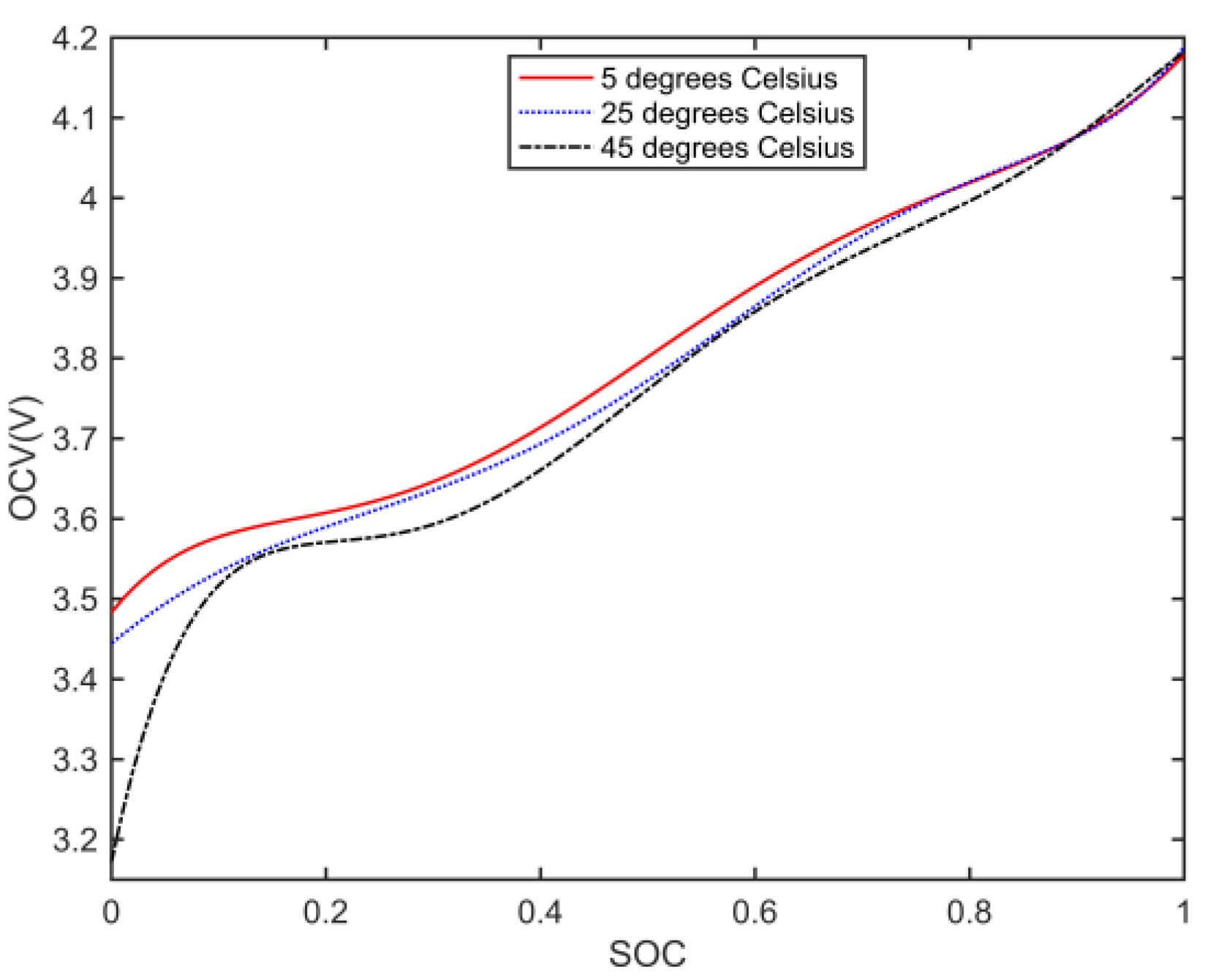
In practice, the LIBs serve in a complicated condition, and the parameters of the 2RC ECM can change greatly due to age effect or varying ambient temperature. The observer should have good performance in terms of robustness against parameter disturbances. In this section, a series of experiments using the procedure described in Section 2.2 were implemented under 5, 25, and 45 °C, respectively.

Table 6. Capacities and parameters of equivalent circuit model (ECM) under different temperatures.

Temperature (°C)	5	25	45
Capacity (Ah)	1.86	2.05	2.16
Ro (Ω)	0.07846	0.03417	0.02802
R1 (Ω)	0.03811	0.02221	0.01828
R2 (Ω)	0.04604	0.01902	0.00338
C1 (F)	2040.80	1498.26	1555.99
C2 (F)	19,450.10	65,453.28	123,611.83

lists the capacities and parameters of ECM for the battery under these temperature conditions. Figure 16 dipicts the relationship between the OCV and SOC under these conditions. We can see that the characteristics of the LIB changes greatly with the change of ambient temperature.

The New European Driving Cycle (NEDC) profile is applied in this experiment. Figure 17 shows the current profile under NEDC profile. The SOC estimation results are displayed in Figure 18.

Table 7. Estimation errors under NEDC test for different temperature conditions.

Temperature (°C)	5	25	45
MAE	3.63%	0.89%	1.83%
Maximum error	30.26%	2.68%	7.14%

lists the estimation errors with the proposed observer under different temperature conditions. From Figure 18, it is clear that the proposed observer can remain stable in a wide range of temperature conditions. This indicates that the proposed method is robust against parameter disturbance. However, when the temperature deviates from room temperature, the estimation error increases rapidly, which is especially obvious in low temperature environments. The decline in estimation accuracy attributes to the change of parameters of battery model. One possible solution is adopting an online parameter identification method to obtain the battery model parameters [42,43]. However, this is beyond the scope of this paper.

4.6. Comparison with Extended Kalman Filter (EKF) Method

To further demonstrate the advantage of the proposed observer, the estimation results were compared with that calculated by another well used algorithm, the extended Kalman filter (EKF). Details about EKF can be found in References [19,20,21,22]. The parameters used in EKF method are listed in

Table 8. Values of the parameters used in the extended Kalman filter (EKF) method.

Parameters	Values
P0	[0.01, 0, 0; 0, 0.001, 0; 0, 0, 0.000001]
Q	[0.0001, 0, 0; 0, 0.0002, 0; 0, 0, 0.0017]
R	0.02

. In Table 8, P₀, Q and R represent initialized state covariance, process noise covariance and measurement noise covariance, respectively. The West Virginia Suburban Driving Schedule (WVUSUB) test was applied in this experiment. Its current profile is shown in Figure 19.

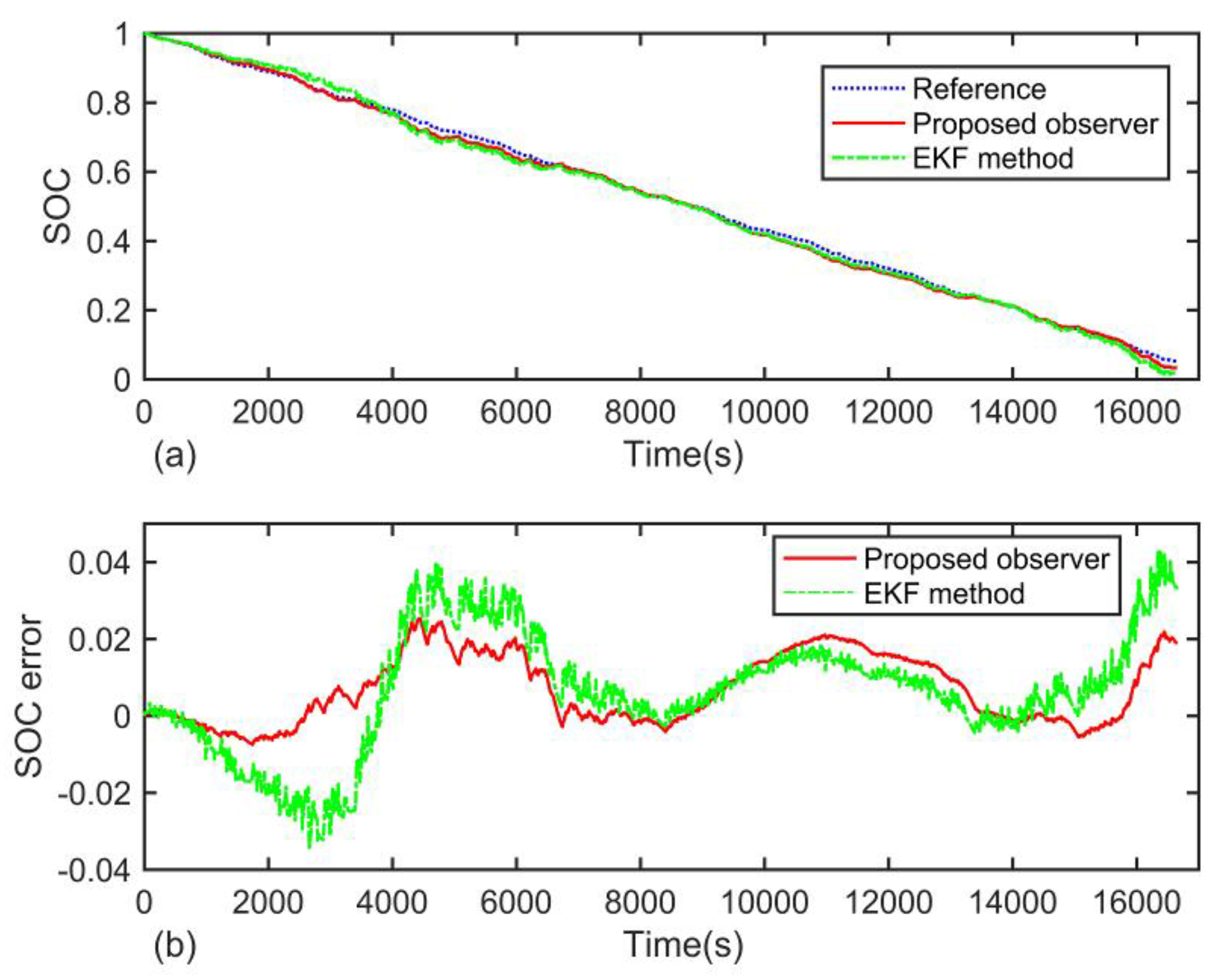
Here, we mainly focus on three aspects of the algorithms, estimation accuracy, computation cost, and convergence rate. In this test, the program running time for each algorithm was recorded to reflect the computation costs of the algorithms. Further, the time for SOC estimation error to converge to 3% for the first time was recorded to evaluate the convergence performance of the algorithms. First, the initial SOC estimation error was set to 0, and the SOC estimation results are shown in Figure 20 and

Table 9. Comparison of computaion cost and SOC estimation error.

Methods	The Proposed Observer	EKF
Computation time (s)	0.1034	0.4184
MAE	0.86%	1.28%
Maximum error	2.53%	4.26%

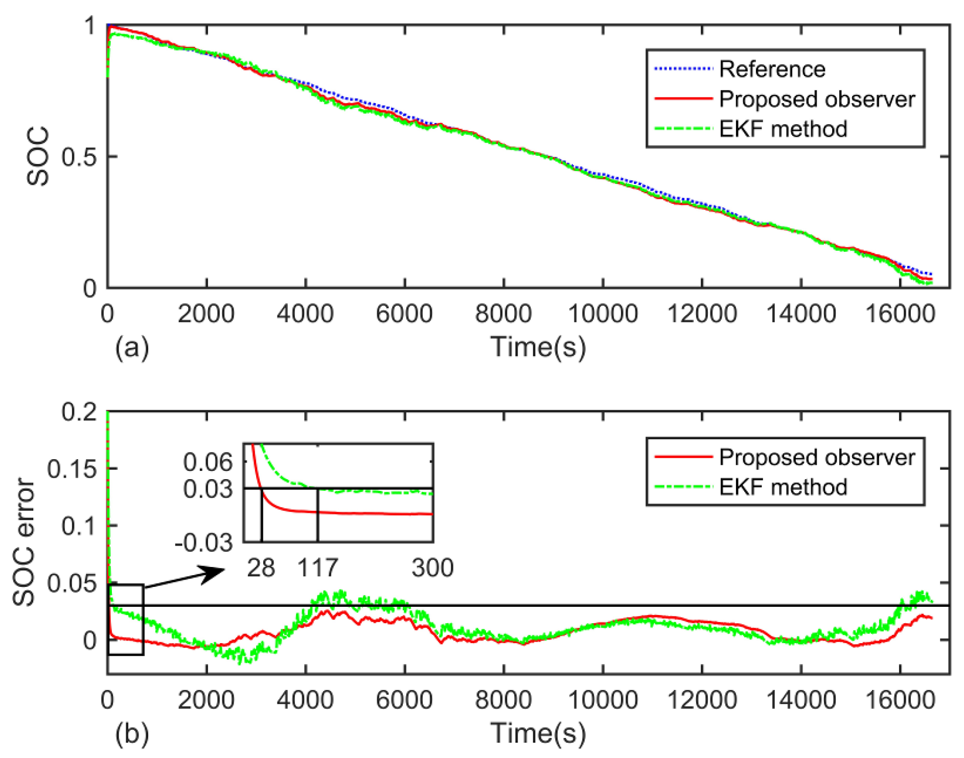
. In Figure 20a, the blue dotted line is the reference SOC. The red solid line and green dash-dotted line represent the ones calculated by the proposed observer and EKF methods, respectively. Figure 20b displays the SOC estimation error. From the results, it is clear that the proposed observer has a notably lower computation cost than the EKF method. Further, the estimation accuracy of the proposed observer is higher than that of EKF method. Second, in order to compare the convergence performance of the algorithms, the initial SOC was set to 0.8—thus, the initial SOC estimation error is 0.2. The estimation results are shown in Figure 21 and

Table 10. Comparison of convergence rate.

Methods	The Proposed Observer	EKF
Convergence time (s)	28	117

.

From Figure 21 and Table 10 we can see that, under the WVUSUB condition, the time that takes the proposed observer to converge to 3% error boundary is 28 s, compared to 117 s for the EKF method. It is clear that the proposed observer has a much faster convergence rate than the EKF method.

5. Conclusions

This paper proposes a novel method for LIB SOC estimation. First, the commonly used 2RC ECM is applied allowing derivation of the state space equations. Next, the exponential fitting method is used to determine the parameters of the model. A six-order polynomial is used to describe the strongly nonlinear relationship between the open circuit voltage and SOC. Then, a novel observer for SOC estimation is proposed. The differential equation theory is utilized to prove the stability of the proposed observer. The FUDS and NEDC experimental results show that the proposed method has good performance in terms of estimation accuracy, convergence rate, robustness against measurement noises, and parameter disturbance. Comparison results with the EKF method also confirm this conclusion. The proposed observer has higher estimation accuracy, and a faster convergence rate than the EKF method, but with lower computational costs. Therefore, the proposed method is more suitable for online SOC estimation.

In Section 4.5, it has been shown that when the parameters change greatly, the estimation accuracy of the proposed observer declines correspondingly. Thus, our future work will be focus on study on combination the proposed method with online parameter identification to improve the robustness against the parameter uncertainty, ambient temperature, age effect, and estimation accuracy.