1. Introduction
Solar-only parabolic trough (PT) thermal power plants have been developed, improving generation over the years thanks to new designs and manufacturing processes. This core block of plant concepts—formed mainly for the solar field, fossil fuel boiler, and power block [
1]—has evolved towards profitable installation by considering different solar radiation areas and different electrical markets [
2,
3]. One of the main developments was the storage system. This has always been present in the concept of solar thermal plants. In fact, as one of the first pilot plants in the world, Plataforma solar de tabernas (PST), was built with 6 KW
e of power generation in Almeria (Spain), starting operation in 1999 with a thermal storage system using direct solar steam. However, until the second half of the decade of the 2000s, there was no continuous investment in thermal energy storage (TES) blocks.
Thermal storage systems integrated into in thermal power plants provide the possibility of developing electrical power generation, improving intermittence, and increasing the profitability of the plant [
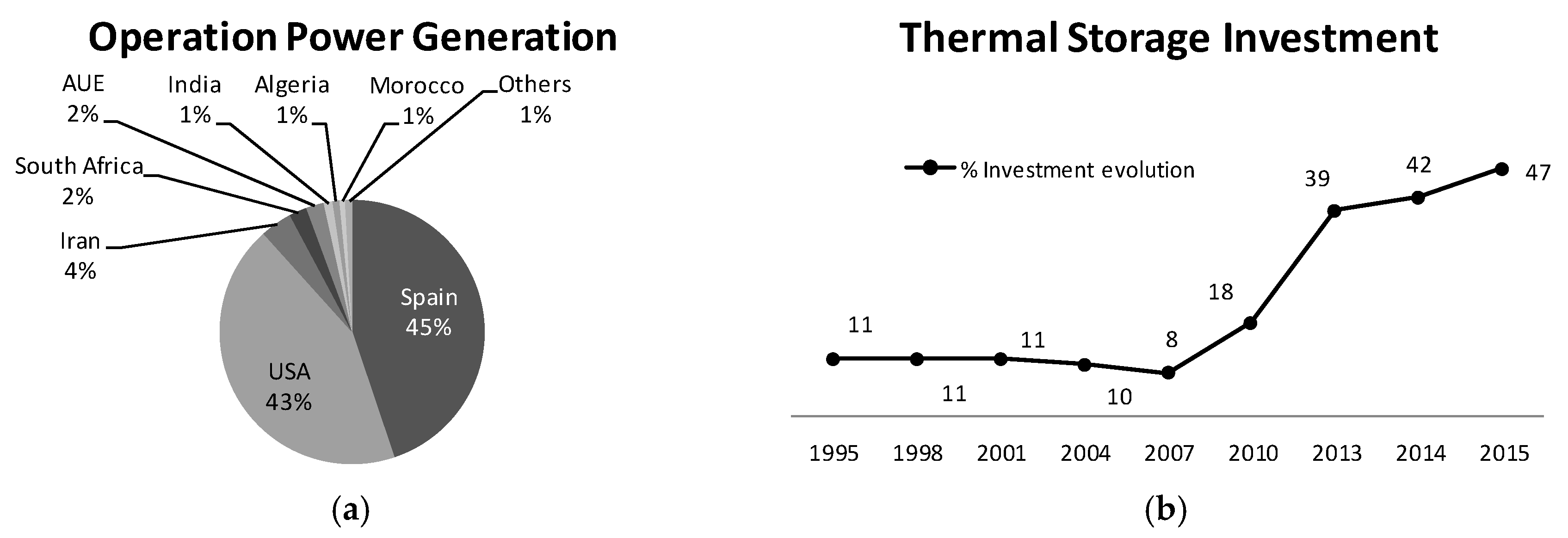
4]. This is an important advantage, offering the opportunity to extend electricity production to periods without solar radiation by adapting the operation procedures. Presently, the total worldwide production using PT solar thermal power plants is over 3.7 GW
e; about 42% of these plants incorporate a TES system, with double-tank molten salt thermal storage systems being the most widespread design concept as of the middle of 2016 [
5,
6] (see
Figure 1). One of the newest PT solar power thermal plants, located in Córdoba (Spain), gives 7.7 equivalent hours of indirect thermal storage with double-tank molten salts. However, double-tank molten salt TES systems involve extremely high investment and maintenance costs. Although the number of hours of direct electric power generation increases notably [
7], the elevated setup expenses, maintenance costs, and long investment payback period give rise to the need to study other TES systems. Heat transfer fluid (HTF) buffering using the solar field as thermal storage system is one of them.
Currently operating PT plants use the solar field as a HTF thermal storage system through an HTF buffer when it is needed, providing short-term storage capacity. This storage capacity is used mainly in two activities. On one hand, this prevents the oil from freezing and thus minimizes the effect of solar resource transient. On the other hand, extra storage capacity for the operation strategy of thermal plants is given. Oversizing the solar field enables the PT plant to increase the operating time at the design point.
The standard working temperature of thermal fluid (synthetic oil) in the solar field of existing plants is 393 °C. The HTF will be sent to the power block until its temperature in the solar field comes down below the minimum operating temperature (380 °C). An increment in the temperature of the thermal fluid achieves enhanced storage capability. This can be achieved by increasing the temperatures in the loops assigned to HTF storage to nearly its maximum operating temperature, 420 °C; or as a more profitable option, by working the entire solar field at this temperature. Long-term tests on the studied plants currently in operation have demonstrated that firstly, degradation for HTF at a circulating temperature of 420 °C is not significant; and secondly, no alteration in the integrity of the solar field has been evidenced.
It is possible to create storage systems with higher equivalent capacity (hours of thermal storage) than standard ones. HTF buffering consists mainly of using the overflow tanks, circulating pumps, HTF, and piping lines of the solar field as a thermal storage system. Once the operation intervals of each device involved in HTF buffering were analyzed, the security operation intervals of each device were been obtained without device arrangements. This analysis lets us determine the optimal strategy of operation using the common upper limits of the HTF buffering devices involved. During the nominal plant activity at sunrise, solar radiation is projected on the concentrating PT, where the direct normal irradiance (DNI) into thermal energy is transformed, heating the circulating working fluid in the solar field, which is conducted to the power block formed by a regenerative Rankine cycle used for electrical power generation. For periods of time apart from sunrise, even with shadows or partial overture, the system maintains the HTF in circulation into the solar field buffer for as much time as needed. The HTF buffering is restored using the thermal energy surplus in the solar field.
The solar multiple (SM) is defined as the ratio between the thermal power produced by the solar field at the design point of the power plant and the thermal power required by the power block at nominal conditions [
8]. Therefore, the higher limits for solar field operation are determined by the SM of the power plant. However, this HTF buffering novel strategy using the common upper limits lets us improve energy production with the same solar radiation. The HTF buffering operation improves the generation curves in accordance with the market dynamics, increasing 3% through 12.5% of thermal energy for a given SM.
In reference to investment costs, it is known that for solar-only plants, the solar field represents the greatest investment [
9]. For this reason, in other work [
8] SM optimization is described. However, molten salt storage block investment plays an important role in the overall plant cost. Considering a value of SM of 1.4 and 3 h of thermal equivalent storage, double-tank molten salt cost increases the plant investment by 9.15% [
10], representing a total of 19.20% of plant investment for equivalent storage sizes up to 7 h.
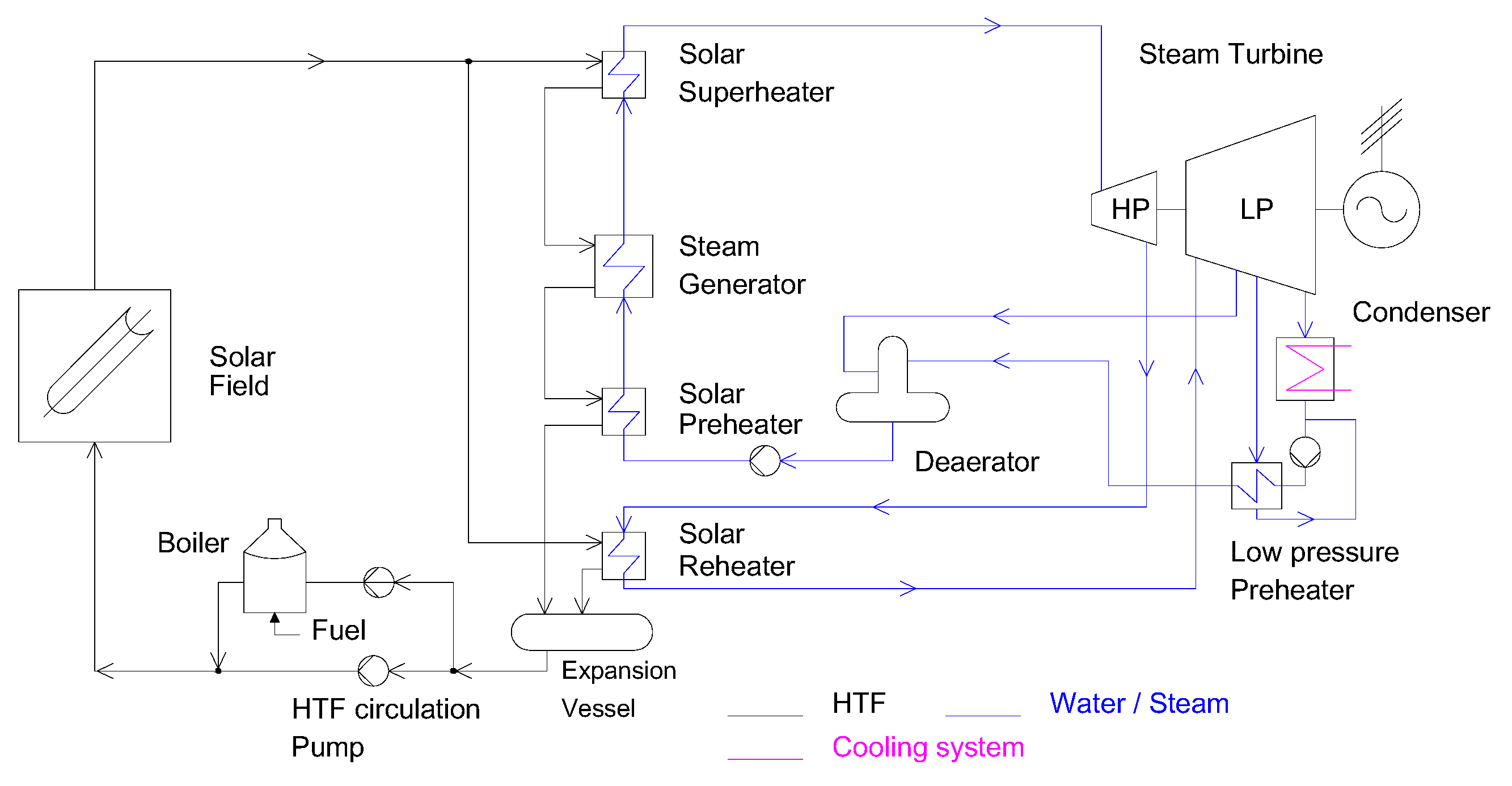
In the study of the HTF buffering TES system oversizing the solar field, a scheme of a solar thermal power plant is shown. An HTF buffering thermal storage system has been simulated using a currently operating plant model site in the south of Spain.
Figure 2 shows a scheme of a solar-only PT power plant as the basis of this work. This large capacity model is described to present a thermal storage scheme as an alternative to presently operated storage systems. The plant model, database, and design-point conditions refer to the operated PT previously mentioned [
11]. The quantification of variables, solar field dimensions, SM value, fired boiler, power block, and design-point conditions setup have been defined, taking the data from this real PT plant. The plant nominal electric power is 50 MW
e to comply with the Spanish renewable energy production law for concentrating solar power (CSP) plants [
12]. Using the PT plant configuration mentioned before, a simulation model has been created considering the period of one year as a reference pattern. Thermal systems used in the models have been obtained from the PT power solar thermal plant.
Techno-economic assessment of HTF buffering for TES in the solar field of PT power plants is the main objective of this work, based on a real thermal power plant.
3. Operation Management and Solar Thermal Plant Model
3.1. Annual Management Performance
All values of SM according to the annual electricity production have been calculated. This electrical power generation of the PT power plant is determined by the normal direct radiation values in direct dispatching, in addition to the derivative of TES in the solar field due to such solar radiation. Annual plant analysis was performed using a mathematical model. This model has been developed based on the ©THERMOLIB library (Aachen, Germany) [
25]. A parallel simulation environment has been created in which data of provided solar radiation were introduced. The combined model is adapted to the characteristics of the proposed plant. The plant operation management is mainly based on four factors. Firstly, the nominal operation period is the time in which solar radiation above the minimum needed for the focused solar collectors provides enough heat to transfer the HTF to the power block. Second, the HTF buffering consigned by the estimated TES start time of the collectors is given by the estimated hourly values of direct normal radiation plus the estimated thermal capacity dumping period to the power block for electricity generation. Third, the fossil fuel boiler supports the plant operation at partial loads and for the plant cold starting. The fourth factor is total computation of the power block production hours in the grid coupling.
These factors, as well as the global daily efficiency, vary as the chosen operating strategy does, hence the importance of selecting the most appropriate operation strategy. It determines the way in which electricity power is produced [
26]. Management operation performed by an optimization function is shown in the next section.
3.2. Plant Model
The reference values given in
Table 2 are extracted from a real plant with coordinates 37°45′ N and 5°3′ W. These data are used in the plant model development based on the scheme of the solar-only PT powered thermal plant in
Figure 2. The mathematical model of the PT plant shown in
Figure 2 is used in a parallel simulation scenario with two models of power plants. A first scenario plant model is without TES; and a second one includes TES with HTF buffering in the HCE. Within this second scenario, a first stage considering the nominal SM of the plant has been simulated and the results are used for validation using data from the real plant. Different simulations of the plant according to six different values of SM have been performed.
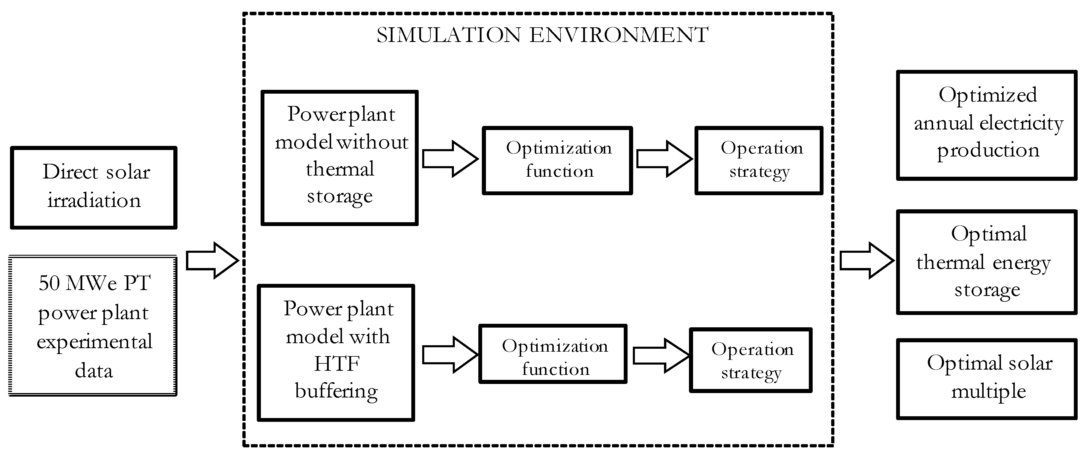
The structure of the simulation environment is presented in
Figure 5. The data acquisition program including economic parameters, HTF technical characteristics, and geographical and solar field data runs in the first instance; the optimization program is executed in parallel for each scenario of the plant described above.
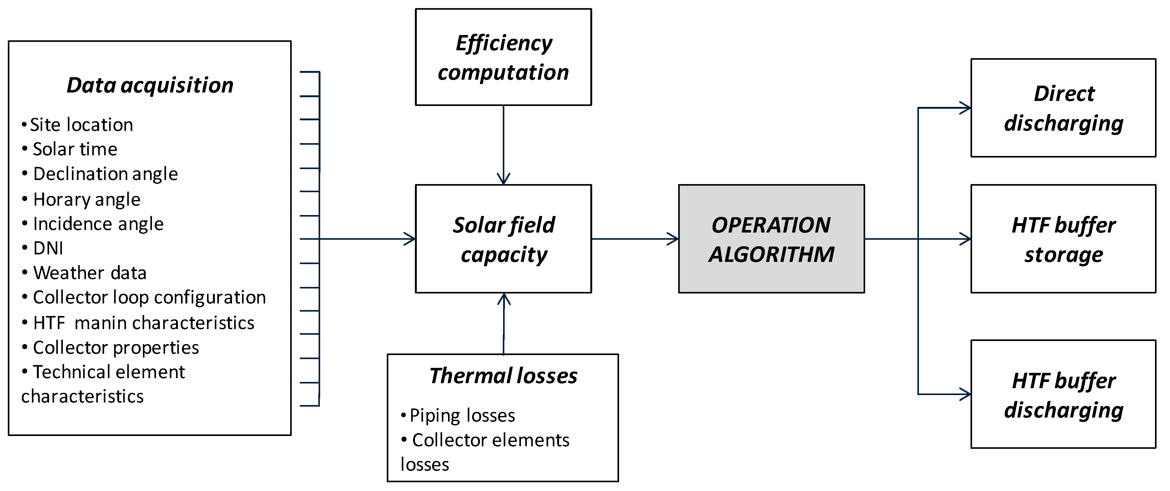
Figure 6 shows the flow chart in which the solar field optimization algorithm for direct discharging and HTF buffering TES has been developed. The input data values, as 8760 dimension vectors, are introduced in a data acquisition module. The restrictions of total stored energy, maximum power generation, SM capacity, and HTF maximum temperature are introduced in the algorithm operation block. The operation algorithm detailed in
Figure 7 allows us to obtain the optimized values for electricity.
The set of tabulated data are grouped and represented by a function that provides the results of computation. The solar collector algorithm used is obtained from a functional block responsible for collecting the solar radiation depending on the time and day of the year, from the data of direct normal solar radiation per unit area introduced from a table of external data.
The set of the solar field loops is modeled using a main basic unit affected by a linear operational amplifier at its input, which is replicated many times as available collectors in the solar field. The relationship between the number of collectors and the solar radiation received (global defocused model) is considered linear.
Simulation models run based on the results of the optimization function. These are:
- (1)
PT solar thermal power plant model with direct discharge, design set SM, and without a TES system in which electricity generation could differ beyond the thermal inertia of the system itself.
- (2)
Plant model with direct discharge, nominal SM, and without TES as described in the previous point, excepting the use of the HTF restraint systems as an energy buffer which would increase the solar field thermal inertia, obtaining a TES equivalent to several hours of electrical power generation, with a cost for thermal storage being rather small compared with other storage systems.
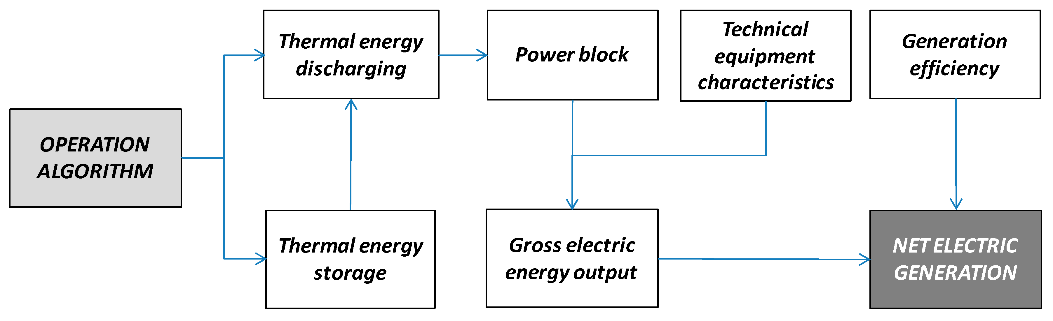
The plant operation algorithm defines the thermal energy sent to the power block, storage in the solar field, HTF buffering discharging, or a combination of both direct discharging and buffer storage. The gross electric energy generated is affected by the technical characteristics of the power block and electric generator elements. Finally, net electricity generation is the gross energy production subtracted by generation efficiency.
Figure 7 shows the functional unit for power block and net electricity generation models.
3.3. Model Validation
Once the description of the model plant was designed and its components were completed, the validation of the model simulation was performed by a reference data set from the solar power plant origin of this study, located at the coordinates 37°45′ N and 5°3′ W. The validation scenario chosen is a nominal condition solar-only plant (solar multiple = 1.2), without TES, and considering that the gas boiler is stopped. Solar radiation lower than 350 W/m2, about 5922 h per year, is not considered enough to operate the power block and turbine. In contrast, with radiation higher than 650 W/m2, about 370 h per year, HTF fluid always reaches the highest design point temperature, 393 °C, so as blur the solar field collectors is forced.
Validation of the mathematical model has been carried out by means of a bin hours method. A comparative analysis has been made taking into account the operating values. This method quantifies —by intervals—an absolute variable, which in our case is the direct solar radiation in the solar field per square meter. After grouping the direct normal radiation in intervals where the radiation received with the annual hours as part of each interval, the comparison between physical parameters of plant with those obtained by the model simulation is undertaken.
For the solar plant validation, HTF fluid parameters at the inlet superheater heat exchanger have been determined as the most significant features. Flow rate, temperature, and pressure values have been taken from the superheater inlet plant sensors and compared with the ones taken from the simulation model. One hundred measurements of solar radiation have been carried out for each parameter at the superheater inlet.
HTF temperature tends to be a fixed value along the plant operation in order to get the maximum efficiency. HTF fluid pressure keeps constant; expansion tanks maintain the fluid pressure within the solar field loops, helping to balance the system. Therefore, the plant makes continuous adjustments on the HTF fluid flow, trying to get the optimal fluid conditions at the power block input.
Table 3 shows the results of the HTF mass flow and temperature-averaged data series comparison using a bin hours yearly interval schedule. The 95th percentile applied to the results allows the statistical adjustment needed for data study and subsequent result validation. Thus, the harmonized results displayed show the concordance between the plant data and the model data. The uncertainty of the temperature is considered to be ±1 °C, and ±0.2 kg/s is the uncertainty of HTF mass flow in the real plant data, both given through metering devices. Data in
Table 3 shows that, along low irradiance periods, the HTF temperature is below the set point. HTF mass flow varies widely from its highest value of 1400 kg/s with maximum solar radiation to the minimum value of 502 kg/s with lower solar radiation.
4. Heat Transfer Fluid Thermal Energy Storage Analysis as a Function of Solar Multiple
The appropriate SM value is based on a set of variables properly adjusted to each individual solar thermal power plant. For direct dispatching plants without TES, these variables are mainly the solar field components and size, plant location, and design conditions. In plants with any thermal storage system, the design’s SM should be enough to offer a thermal energy surplus to the thermal storage block. The target of this study is to store thermal energy in the solar field, where the piping system acts by itself as a TES. For that proposal, system device losses in the piping system, collector area, circulating pump block, and plant performance in nominal operating conditions must be taken into account.
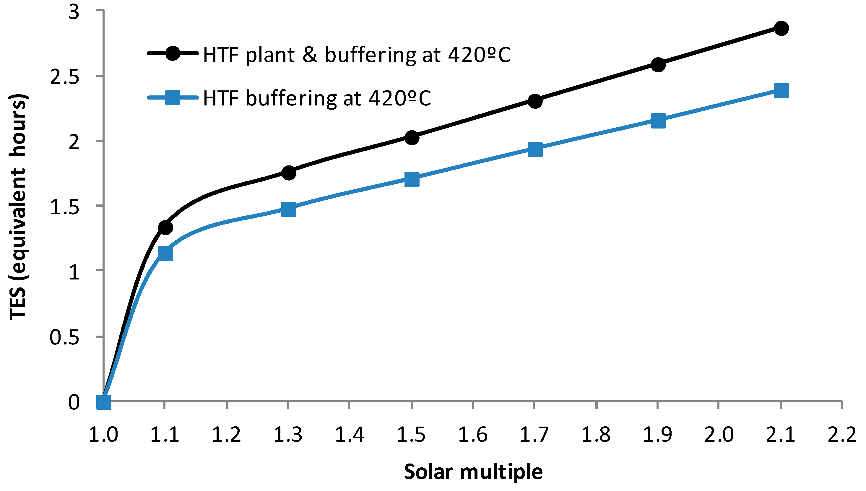
As shown in
Figure 8, two working scenarios for the annual equivalent HTF buffering thermal storage energy as a function of SM have been carried out. The first scenario studies the equivalent hours of TES, considering an HTF buffering temperature of 420 °C in the storage loops and 393 °C (standard HTF temperature) for the rest of the solar field and power block HTF temperature input. A second scenario considers an HTF temperature of 420 °C in the whole solar field, including the storage loops and the ones working for direct dispatching. Due to an SM higher than 1, during direct dispatching the PT plant can produce the nominal power while the HTF system is recharged by the solar field. During scarce or null radiation periods, the power block takes the thermal energy from the solar HTF buffering, reducing its temperature until maintenance limits.
The first scenario is mainly focused on the operation and maintenance plant modifications. The second scenario needs, besides the plant structural modifications of the first scenario, a special HTF for long round working periods at 420 °C.
Figure 8 plots how the amount of equivalent thermal energy stored in the second scenario, where the HTF plant and the buffering are at 420 °C, which is proportionally higher than in the first scenario for all values of SM considered. Thus, second state will be used as a basis of this work.
For the present study, six values of SM have been considered. Each SM value leads to its corresponding TES as well as to different sizes of solar fields. The collector area varies depending on the solar field size. Averaged DNI values and plant operability vary depending on the time of year. Finally, TES and thermal losses in the piping line vary depending on both the size of the solar field and the time of year. Annual HTF buffering thermal storage size, thermal losses in piping line, and solar field size have been calculated as a function of SM.
Table 4 shows the average annual values of TES and solar field oversize for different SM values. The increase in SM increases the capacity loss in the piping. This is due to the increasing number of solar collectors and the greater number of operation hours of the solar field. Thus, thermal energy losses to be considered are both losses during the daytime operation and the corresponding HTF buffer discharge during overcast sky or sunset periods. The TES in the solar field increases as the SM is greater. Full load TES data in
Table 4, both in daily absolute terms (MWh
th) and equivalent hours of thermal storage, can be used for a comparative study of other thermal storage systems, serving as a foundation for future work.
5. Economic Analysis
Economic analysis is focused on the most profitable operation situation, which is the second scenario described in the previous section. The average lifetime levelized cost of electricity (LCOE) is determined for different values of SM [
27]. An economic assessment which has been used to compare the costs of electric energy production according to the different values of SM is considered. The costs of fossil fuel to feed a gas boiler have been considered in our conception of LCOE. Equation (3) is used to obtain the value of LCOE for the different considered solar power plant configurations:
The capital cost in the year
t is calculated in Equation (4):
The capital recovery factor is calculated according to Equation (5):
where
is the debt interest rate;
is the depreciation period;
is the annual insurance rate;
is the values buzzer along the depreciation period;
is plant investment cost;
is the combined fix and variable operation and maintenance cost in the year t which can be calculated as
;
is the operation and maintenance cost referenced to the plant capacity;
is the operation and maintenance cost referenced to the electric energy production;
is the fuel consumption cost in the year
t; and
is the net electric energy production in the year
t.
Main data assumptions used for economic analysis are shown in
Table 5. The main data baseline has been taken from [
28]. Cost due to investment, fixed and variable operation, and maintenance and fuel consumption are different according to the SM dimension as this value directly affects the size of the solar field, the amount of electricity generated, and fuel consumption. The data in
Table 5 have been estimated considering a depreciation period of 25 years and a debt interest rate of 8.0%.
Economic results for six values of equivalent full load TES are shown in
Table 6. For the power block, 40% average conversion efficiency has been considered, as well as 20% of thermal capacity fraction for standby and startup. Sensitivity parameters analysis shows that the investment cost increases with the size of the solar field due to the increased in the number of collectors such as the pumping system and its auxiliary elements. Meanwhile, the cost of operation and maintenance are also enhanced by the oversized solar field, mainly due to the increased number of maintenance operations caused by the increased of the solar field size and the plant operation hours.
The gas boiler’s main use is based on the first startup operation of any day as well as for covering the solar radiation fluctuations along the day. Thus, fuel consumption costs increase as the TES does; this is due to the fact that, as the solar field size is greater, a higher boiler runtime is needed to retain the HTF temperature within the correct margins for performance over time.
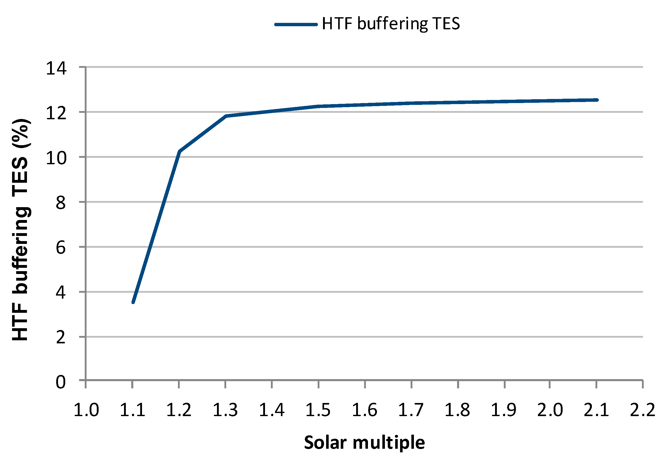
Figure 9 shows the HTF buffering thermal storage as a function of the SM. The curve implies high efficiency of HTF buffering considering a SM greater than 1.3.
As commented in other works, for solar-only plants, defocusing collectors are used when the SM is higher than one [
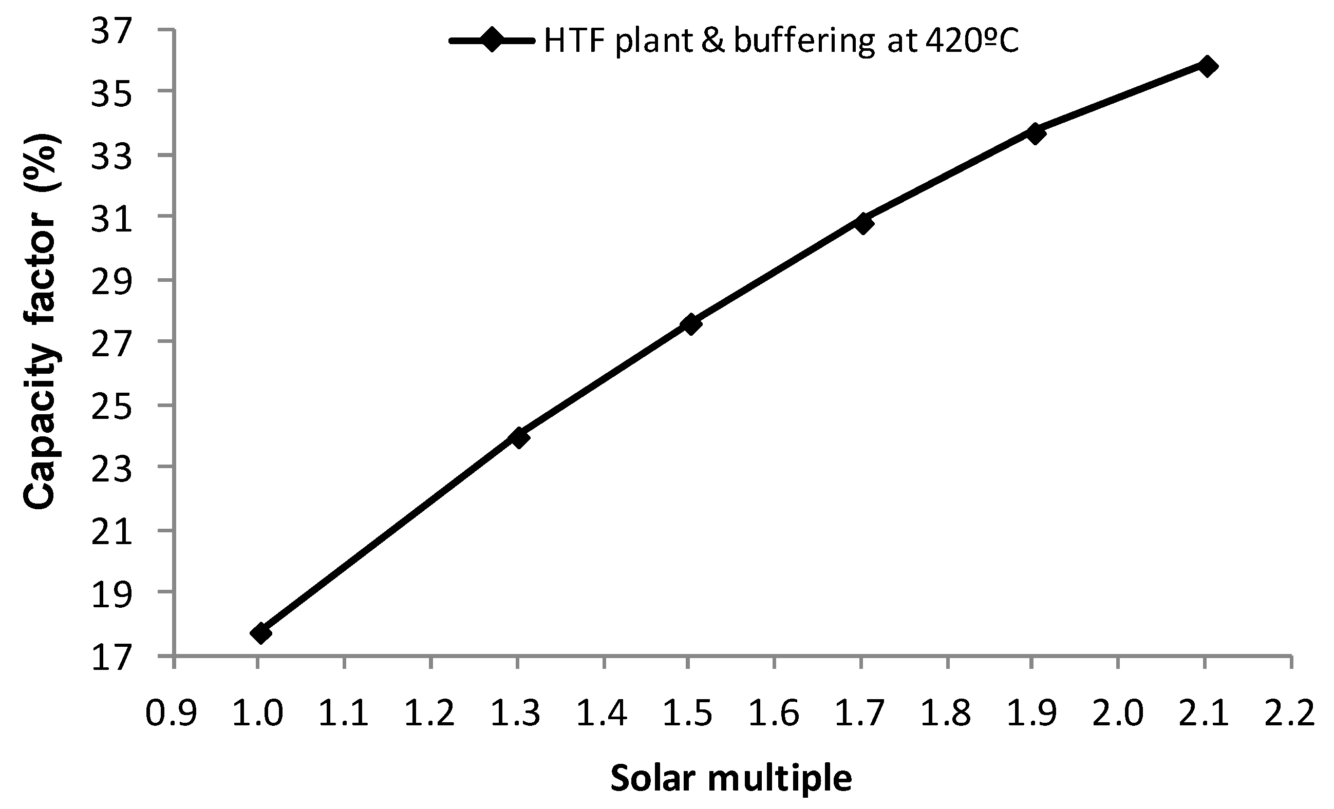
30]. Furthermore, an SM of about 1.3 is found to minimize the LCOE. As shown in
Figure 10, HTF buffering thermal storage extends the plant operating time, thus increasing the capacity factor. For common design plants with SM = 1.3, HTF buffering enables a capacity factor of 23.65%. This value is significantly higher than plants with direct discharging traditional operating mode [
9], where capacity factor is around 16%. The best results are achieved for solar higher multiple values where the capacity factor reaches levels of 35.85% for SM = 2.1.
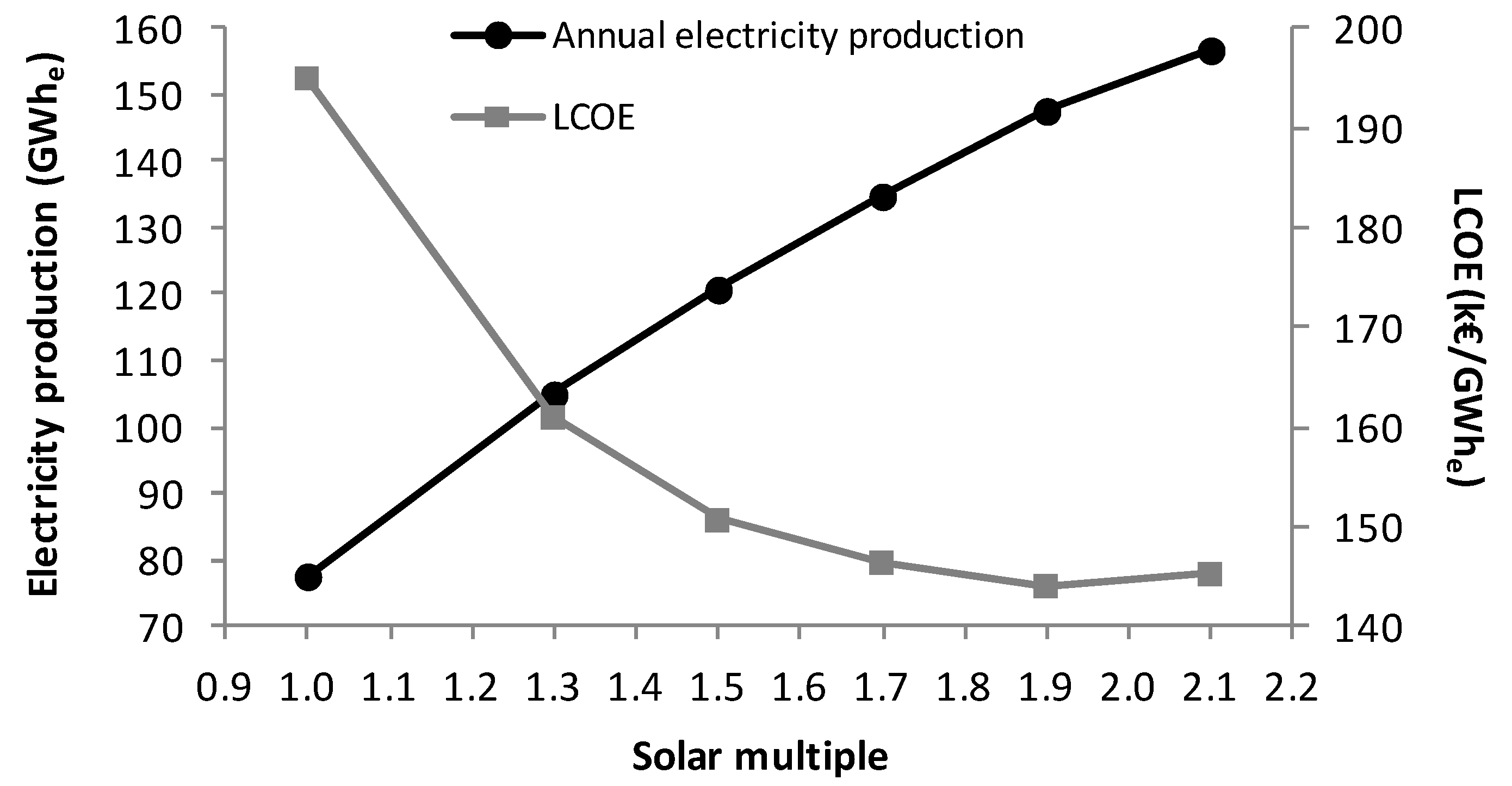
As well as improving the capacity factor, HTF buffering enables diversion of the energy into thermal storage as shown in
Table 6. The electricity production and the LCOE evolution values according to SM are shown in
Figure 11. The electrical generation increases at the same time as the field size does, increasing by 156.73 GWh
e with SM = 2.1.
However, the LCOE decrease reaches a critical point at SM = 1.9 and 144.05 k€/GWhe, with LCOE being 145.23 k€/GWhe for SM = 2.1. It breaks its downtrend and tends to increase. Hence, plant electricity production is not able to offset the investments in the solar field and O&M for SM over 1.9. This is mainly because the collector system is not suitable for very long-term storage capacity when sufficient insulation is not provided, and pass heat losses make the HTF temperature decrease gradually until reaching non-operational temperature points.
The optimal thermal storage value is the one which obtains the highest electricity production with a minimum cost of electricity. Electricity market price factors and grip operation strategies have not been taken into account in this study, providing a basis for further works. According the parameters considered, an SM value of 1.9 is the most profitable size in order to obtain the maximum capability to the thermal power plant. Values of SM below 1.3 and above 1.9 carry a non-trend cost of energy decreases, as shown in
Figure 11, leading to collector configurations far from the optimal solar field design.
6. Discussion
As shown in
Figure 10, an increase of annual electric energy generation gives rise to higher solar-to-electric efficiency as the SM enhances. With respect to the LCOE, it is noted that its value decreases when increasing the value of the SM up to SM = 1.9, where trends towards growth are mainly influenced by the high cost of the solar field investment and solar field performance loss, as seen in
Table 6.
Figure 11 represents the annual net electricity production and LCOE as a function of the SM, where SM = 1.9 obtains the maximum capability according to the plant capacity (50 MW
e) and location (between parallels 37 N–40 N) which are basic to this work. For a solar field size of 1.9, electricity generated and LCOE are 147.61 GWh
e and 144.05 k€/GWh
e, respectively. These values of yearly generated energy and LCOE have been improved 8.54% and 6.01%, respectively, in comparison with the values from the power plant simulated without HTF buffering.
The results obtained are given without considering methods of operation of the electricity market. Thereby, a constant electricity demand has been taken without the electricity price being affected by incentives from the market. Besides, the consequences associated with the solar field oversizing in terms of heat losses, pressure drop and pump unit size increments in the pipe line, efficiency of the whole system, and the useful operating hours of the gas boiler have been considered. The method described in this study can be used as a basis for analyzing the HTF buffering performance of specific plants, either currently operated or at the design stage; with each adapted to its SM singular value.
7. Conclusions
An innovative and available thermal storage methodology using the solar field as a heat fluid buffer has been carried out. As a first scenario, a 50-MWe solar-only PT power thermal plant model was created, corresponding to a specific area located between the parallels 37 N and 40 N.
The plant model, using different nominal preset SM values, was simulated for a period of one year as a direct dispatch from the solar field to the power block, using the solar field as TES through an HTF buffer. Using currently operated plant data acquisition, the model has been validated and data have been calibrated.
The second scenario proposed increased the HTF working temperature in the solar field to 420 °C. This working temperature is taken as the basis for further calculations, allowing higher throughput in the TES. The effect of different SM values on the electricity power generated, its equivalent hours of TES, capacity factor associated, and LCOE have been analyzed. The increase in the operating and maintenance costs and a significant increase in losses in the piping line are offset by the improved fostered energy storage.


