Impact of Stress-Dependent Matrix and Fracture Properties on Shale Gas Production

Abstract

Unconventional shale gas production is often characterized by a short period of high production followed by a rapid decline in the production rate. Given the high costs of hydraulic fracturing and horizontal drilling, it is critical to identify the mechanisms behind the production loss. The existing shale gas production models often assume constant matrix permeability. However, laboratory observations show that matrix permeability can decrease significantly with increasing effective stress, which highlights the necessity of considering the stress-dependent properties of shale matrix in production analysis. Moreover, the compaction of pore space will also increase the matrix permeability by enhancing the gas-slippage effect. In this paper, a matrix permeability model which couples the effect of pore volume compaction and non-Darcy slip flow is derived. Numerical simulations are conducted to understand the role of matrix permeability evolution during production. Changes of fractures’ permeability and contact area during depletion process are also taken into account. The results indicate that the loss of fracture permeability has a greater impact at the early stage of the depletion process, while matrix permeability evolution is more important for the long-term production.

1. Introduction

A significant amount of natural gas in the United States is produced from shale gas reservoirs. Although the initial production rates might be high for shale gas wells, the rates decline steeply [1,2], which significantly affects the economics of many shale gas projects. Therefore, it is of great importance to identify the mechanisms responsible for the rapid production loss for shale gas reservoirs.

In shales, the transport processes take place on scales covering several orders of magnitude. These processes range from the slip flow which occurs on the nanometer scale, to fracture flow which takes place on the centimeter scale. The slip flow, also known as Klinkenberg effect [3,4], occurs when the mean free path length of a gas molecule is on the same order of magnitude as the pore size. In this situation, the gas molecules might be accelerated along the flow path which results in an increase in the apparent permeability. The slip flow and the compaction of pores have been studied independently in literature. However, because the strength of gas slippage is related to the size of the pore-throat, the pore size reduction caused by compaction will also influence the slippage process. It has been proved by coal experiments that a strong coupling effect exists between the pore compressibility and the gas slippage [5]. Thus, it is necessary to build a coupled permeability model to combine the gas-slippage effect and pore size compaction for unconventional reservoirs.

In addition to the matrix gas flow, the fracture flow is also critically important in unconventional reservoirs. The conductivities of fractures were found to be very sensitive to the applied effective stress based on the experiment results [6]. The impact of stress-dependent fracture conductivities on gas production has been studied using numerical simulations [7,8]. Besides, the contact area between matrix and fractures will affect gas transport between matrix and fractures. For example, Huo and Benson [9] reported a loss of contact area of opened fractures by scanning shale samples layer by layer. Later, Pyrak-Nolte and Nolte [10] conducted numerical simulations on fluid flow through porous media and the contact surface area was found to decrease with increasing effective stress as well. However, a mathematical model that represents the impact of contact surface area loss on shale gas production has not been investigated yet.

In this study, we develop a matrix permeability model which couples the poro-elastic and the gas-slippage effects. The impacts of stress-dependent fracture and matrix permeabilities on shale gas production are investigated to understand the relative importance of these effects. The mechanism of fracture-matrix contact area loss is also discussed and integrated into the stress-dependent model.

2. Model Description

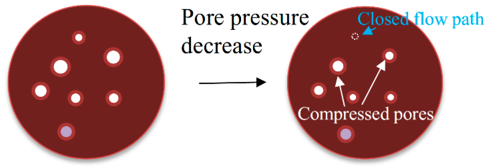
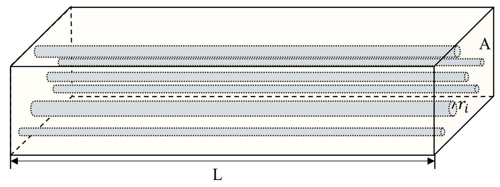
2.1. Stress-Dependent Matrix Permeability

As the effective stress increases, both the matrix permeability and porosity will be reduced due to the compaction of pores (Figure 1). The dependence of matrix permeability on effective stress can be described as a poro-elastic effect which has an exponential form [11,12]:

$$k_d=k_{d,0}{e}^{-c_m{\sigma }_{eff}}=k_{d,0}{e}^{-c_m\left({\sigma }_c-x{p}_f\right)}$$

(1)

where $k_d$ is the matrix permeability at low Knudsen number (<0.01, Heller et al. [13]) when only Darcy flow occurs, subscript d indicates Darcy flow, $c_m$ is the poro-elastic coefficient, $x$ is the Biot’s constant, ${\sigma }_c$ is the confining stress, $p_f$ is the fluid pressure, and $k_{d,0}$ denotes the matrix permeability under zero effective stress.

We assume that the pore space in shale matrix consists of a series of parallel tubes with varying radii as shown in Figure 2. The intrinsic permeability, $k_{\mathrm{int}}$, of a cylinder tube with the radius of $r$ is given by [14]:

$$k_{\mathrm{int}}=\frac{r^2}{8}$$

(2)

Based on Equation (2), the apparent permeability (permeability measured by total flux) of the shale matrix system shown in Figure 2 can then be expressed by:

$$k_d=\frac{\pi }{8}\frac{{\displaystyle {\sum }_1^N{r}_i^4}}{A}$$

(3)

where r_i is the radius of tube i (i ranges from 1 to N), N is the number of tubes in the matrix, and A is the total area of the cross-section perpendicular to the tubes. The porosity can be written as a function of tube radius as well:

$$\varphi =\frac{\pi }{A}{\displaystyle \sum _1^N{r}_i^2}$$

(4)

By combining Equations (1) and (3), with further assumption that the compressibility, the change of pore radius with per unit increase of effective stress, of each tube is the same, the radius of tube i under the effective stress can be written as:

$$r_i=r_{i,0}{e}^{-\frac{c_m}{4}{\sigma }_{eff}}=r_{i,0}{e}^{-\frac{c_m}{4}\left({\sigma }_c-x{p}_f\right)}$$

(5)

where $r_{i,0}$ is the radius of tube i under zero effective stress, and all the other variables are as defined previously. The compressibility of the pores can then be written as:

$$c_r=-\frac{1}{r}\frac{\partial r}{\partial {\sigma }_{eff}}=\frac{c_m}{4}$$

(6)

The mean free path $\lambda$ of an ideal gas is given by:

$$\lambda =\frac{{\mu }_g{Z}_g}{p_f}\sqrt{\frac{\pi RT}{2M}}$$

(7)

where μ_g is the gas viscosity, Z_g is the gas compressibility factor, R is the universal gas constant which equals to 8.314 J/mol/K, and M and T are the molecule weight and temperature of the ideal gas, respectively. Knudsen number is defined as the ratio of the molecule mean free path to the flow path radius (e.g., radius of the tube):

$$K_n=\frac{\lambda }{r}=\frac{{\mu }_g{Z}_g}{p_{f}r}\sqrt{\frac{\pi RT}{2M}}$$

(8)

By substituting Equation (5) into Equation (8), the Knudsen number can be expressed with the fluid pressure as:

$$K_n=\frac{{\mu }_g{Z}_g}{p_f{r}_0{}^{-\frac{c_m}{4}\left({\sigma }_c-x{p}_f\right)}}\sqrt{\frac{\pi RT}{2M}}$$

(9)

With the decrease in fluid pressure during the production, the Knudsen number will increase not only due to the pressure decline but also due to the shrinkage of the tubes.

In the nanometer-scale pores in shale matrix, the mean free path is comparable with the tube radius. In this circumstance, the gas molecules may slip along the tube which results in an increase in the apparent matrix permeability. A variety of models to correct the permeability with gas-slippage effect have been proposed in the literature [15,16]. Here, the formulation developed by Zhang et al. [17] is adopted and is given by:

$$k_{\mathrm{int},t}=k_{\mathrm{int}}\left(1+c{K}_n\right)$$

(10)

where $k_{\mathrm{int},t}$ is the instrinsic permeability with consideration of gas slippage, c is a constant derived based on the kinetic theory of gases and the value of c is taken as 6 in most situations [17].

By substituting Equations (2) and (9) into Equation (10), for the tube with radius $r_i$, the intrinsic permeability with gas-slippage effect can then be expressed as:

$$k_{\mathrm{int},i}=\frac{r_i^2}{8}\left(1+c\frac{{\mu }_g{Z}_g}{p_f{r}_i}\sqrt{\frac{\pi RT}{2M}}\right)=\frac{r_{i,0}^2{e}^{-\frac{c_m}{2}\left({\sigma }_c-x{p}_f\right)}}{8}\left(1+c\frac{{\mu }_g{Z}_g}{p_f{r}_{i,0}{}^{-\frac{c_m}{4}\left(p_c-x{p}_f\right)}}\sqrt{\frac{\pi RT}{2M}}\right)$$

(11)

By calculating the permeability of each cube with Equation (11), the volumetric flow rate across the cross-section in Figure 2 can then be calculated as:

$$\overrightarrow{Q}=-\frac{{\displaystyle {\sum }_1^N{k}_{\mathrm{int},i}\cdot \left(\pi r_i^2\right)}}{\mu }\nabla p=-\frac{A{k}_m}{\mu }\nabla p$$

(12)

where k_m is the apparent matrix permeability and can be computed as:

$$k_m=\frac{\pi {\displaystyle {\sum }_1^N{k}_{\mathrm{int},i}{r}_i^2}}{A}=\frac{\pi }{A}{\displaystyle {\sum }_1^N\frac{r_{i,0}^4{e}^{-c_m\left({\sigma }_c-x{p}_f\right)}}{8}\left(1+c\frac{{\mu }_g{Z}_g}{p_f{r}_{i,0}{e}^{-\frac{c_m}{4}\left(p_c-x{p}_f\right)}}\sqrt{\frac{\pi RT}{2M}}\right)}$$

(13)

If we assume all tubes have the same radius, the above equation can be simplified as:

$$\begin{array}{l}{k}_m=\frac{\pi N}{A}\frac{r_0^4{e}^{-c_m({\sigma }_c-x{p}_f)}}{8}\left(1+c\frac{{\mu }_g{Z}_g}{p_f{r}_0{e}^{-\frac{c_m}{4}({\sigma }_c-x{p}_f)}}\sqrt{\frac{\pi RT}{2M}}\right)=\\ k_{d,0}{e}^{-c_m({\sigma }_c-x{p}_f)}\left(1+c\frac{{\mu }_g{Z}_g}{p_f{r}_0{e}^{-\frac{c_m}{4}({\sigma }_c-x{p}_f)}}\sqrt{\frac{\pi RT}{2M}}\right)\end{array}$$

(14)

One assumption made in Equation (14) is that the slippage effect can be neglected at the initial pore pressure because the pressure before production is considered high. Only with this assumption, we can use k_d,0 to replace $\frac{\pi N}{A}\frac{r_0^4}{8}$.

According to Equation (14), it is seen that the poro-elastic coefficient, c_m, is an important parameter in controlling the change of matrix permeability during the depletion process. We can also observe that the gas-slippage effect becomes more important as pressure depletion continues, not only due to the decrease in the pore pressure but also because of the compaction of the flow path. The resulting permeability for the fully coupled model could be higher than the model that only considers the poro-elastic effect, especially in the later production stage.

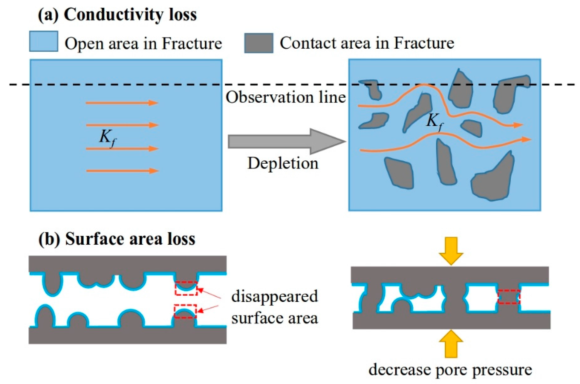
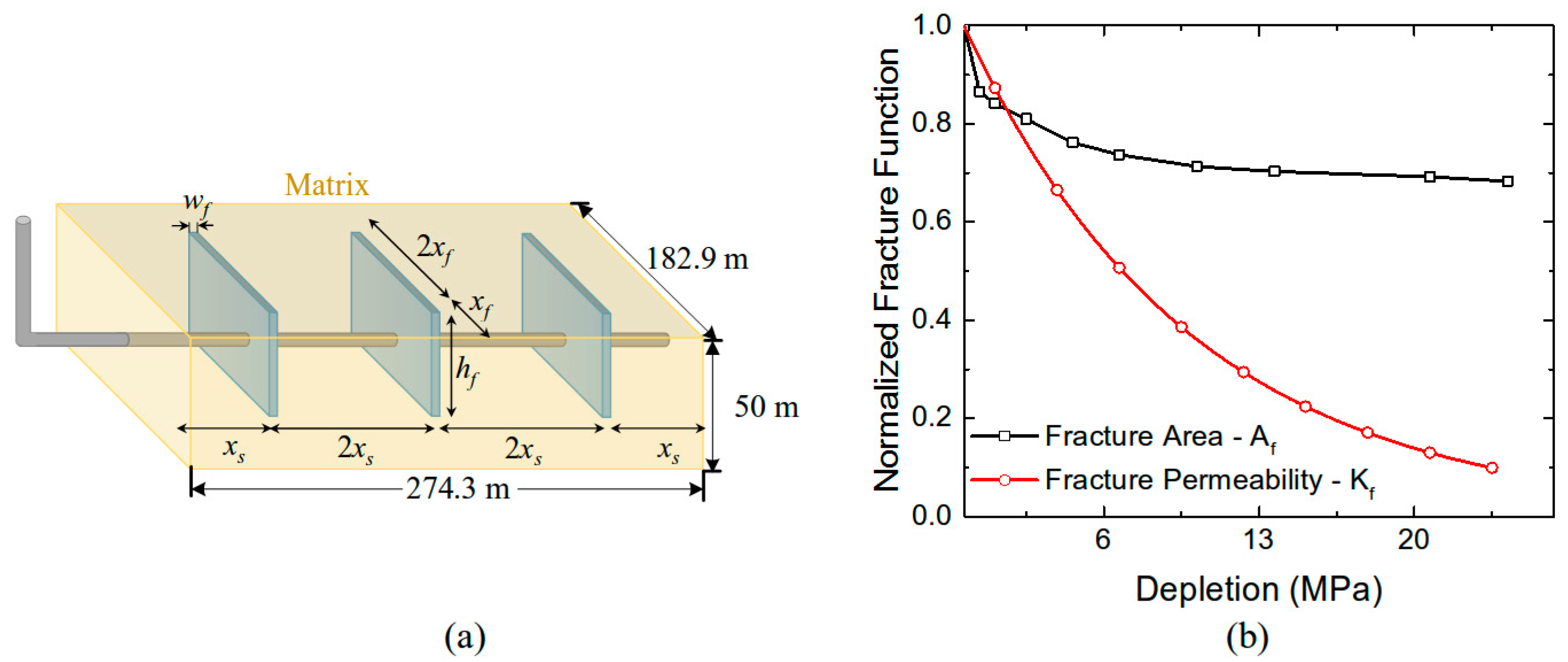
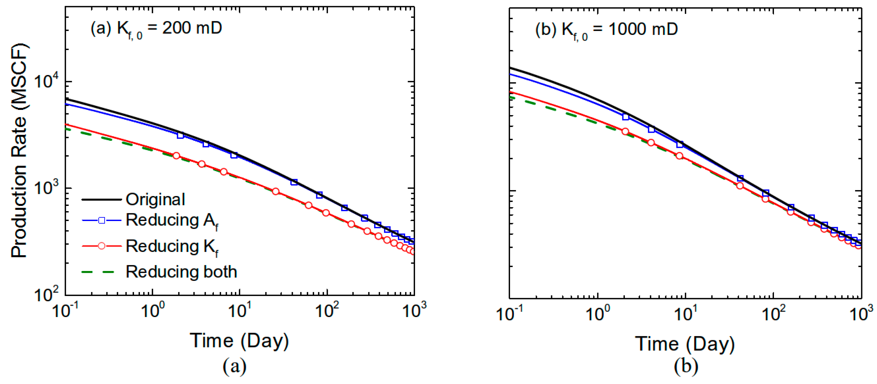
2.2. Stress-Dependent Fracture Permeability and Contact Surface Area

In this work, we consider relatively simple fracture model in which the fracture width is assumed to be constant. With this assumption, the fracture permeability and fracture conductivity can be computed from each other. Therefore, both fracture permeability and conductivity will be used in the following description.

According to Alramahi and Sundberg [18], the impairment of hydraulic fracture conductivity can be attributed to several different mechanisms, including fines migration, proppant diagenesis, proppant crushing, and proppant embedment. Cho et al. [7] conducted an experimental study to investigate the relationship between the natural fracture permeability and reservoir pressure using Bakken core samples. Zhang et al. [19] demonstrated that high proppant concentration was critical to the maintenance of effective fracture conductivity. Suarez-Rivera and Burghardt [6] recreated the hydraulic fracturing process on rock samples and measured the evolution of propped and unpropped fracture conductivity with different confining pressures. In the above work, a strong correlation of fracture permeability with the effective stress has been observed. The correlation can be written as [18]:

$$K_f=K_{f,0}{e}^{-c_f\left({\sigma }_c-x{p}_f\right)}$$

(15)

where K_f is the fracture permeability and $c_f$ is the compliance of the fracture which can be considered as the poro-elastic coefficient of the fractures. In this study, we only focus on the effect of hydraulic fractures. The influence of the natural fractures will be presented in a separate work. The compliance of hydraulic fractures spans a wide range according to the literature due to the variations in proppant embedment and rock properties [6,7]. In the work by Suarez-Rivera and Burghardt [6], the authors reported the measured fracture compliance of approximately 0.11 MPa⁻¹ for propped fractures and 0.34 MPa⁻¹ for unpropped fractures. The c_f measured by Alramahi and Sundberg [18] varied from 0.03 MPa⁻¹ to 0.2 MPa⁻¹ under different proppant embedment situations.

Fracture surface area loss under large effective stress has been observed in previous work [9,10]. The effect of contact area loss is often misinterpreted as the reduction of fracture permeability. In fact, fracture surface loss is a distinct effect which acts by sealing flow exchange area between matrix and fracture. This effect is reflected in the mass transfer term between the matrix and fracture rather than in the flow convection term:

$$\frac{\partial }{\partial x}\left(\frac{K_f\left(p_{f,F}\right)wh}{{\varphi }_f{S}_g{c}_g\left(p_{f,F}\right)}\frac{\partial M}{\partial x}\right)+\frac{\partial }{\partial y}\left(\frac{A_f\left(p_{f,F}\right)k_m\left(p_{f,m}\right)}{{\varphi }_m{S}_g{c}_g\left(p_{f,m}\right)}\frac{\partial M}{\partial x}\right)+q=0$$

(16)

where M is the fluid mass in fracture, w is the width of fracture, x is the direction along the fracture length and y denotes the direction perpendicular to the fracture surface. The first term in Equation (16) represents the flow within the fracture where the fracture permeability and gas compressibility (c_g) are determined by fluid pressure in the fracture, p_f,F. The second term describes the mass transfer between the fracture and matrix. Since the fluid flows from the matrix to the fracture, the stress-dependent properties are calculated using the matrix pressure p_f,m. The symbol $A_f\left(p_{f,F}\right)$ represents the fracture surface area and q is the source/sink term in the fracture.

The difference between fracture permeability loss and fracture surface area loss is depicted in Figure 3. During the depletion, the decrease of fluid pressure will induce fracture compaction, which results in a reduction in the opened space between fracture surfaces as shown in Figure 3a. Due to the loss of available flow path, the flow capacity of the fracture reduces. This phenomenon is represented by fracture permeability loss. Meanwhile, the change of fracture-matrix contact area will affect the flow between the matrix and fracture. In Figure 3b, the light blue curve indicates the fracture-matrix contact area. As pore pressure decreases, a portion of contacted fracture surface area may disappear as depicted in Figure 3b. In our model, this loss of fracture surface area is described by $A_f\left(p_{f,F}\right)$, which monotonically decreases as the pore pressure reduces. In the next section, this fracture surface area loss effect will be simulated as well to quantify its impact on shale gas production.

The above-mentioned models are implemented in the General Purpose Research Simulator (GPRS) developed by the Stanford University Reservoir Simulation Research program (SUPRI-B). GPRS is based on finite volume method and is capable of simulating multiphase, multicomponent flows in porous media [20,21]. In this work, the black oil model with single gas phase is used. The values of matrix permeability, fracture permeability and fracture surface area are updated at each Newton iteration until the convergence criteria are met.

3. Results and Discussions

In this section, we will present the simulation results to demonstrate the impact of the variations of the above-mentioned properties on shale gas production.

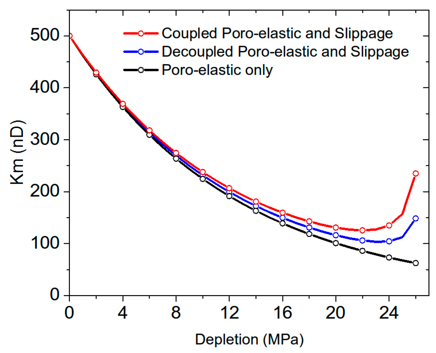
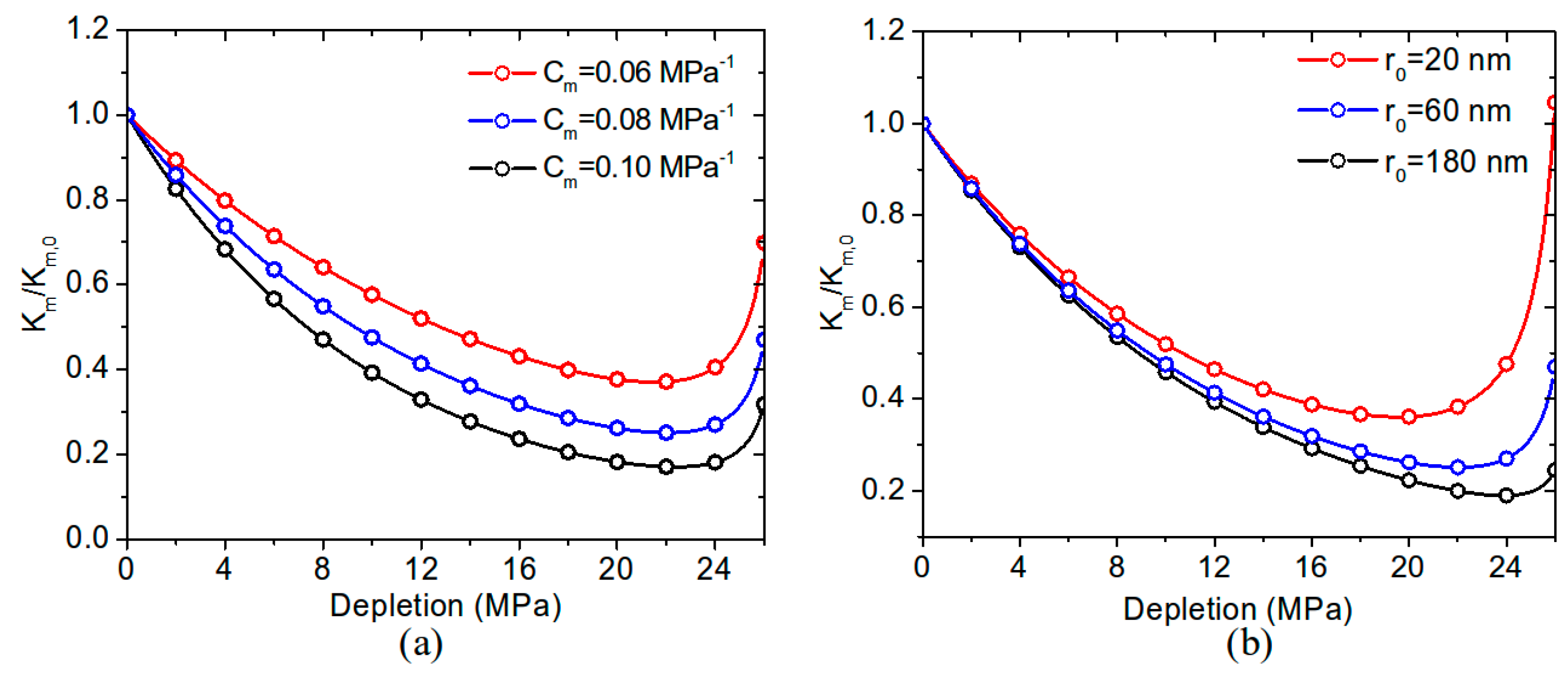
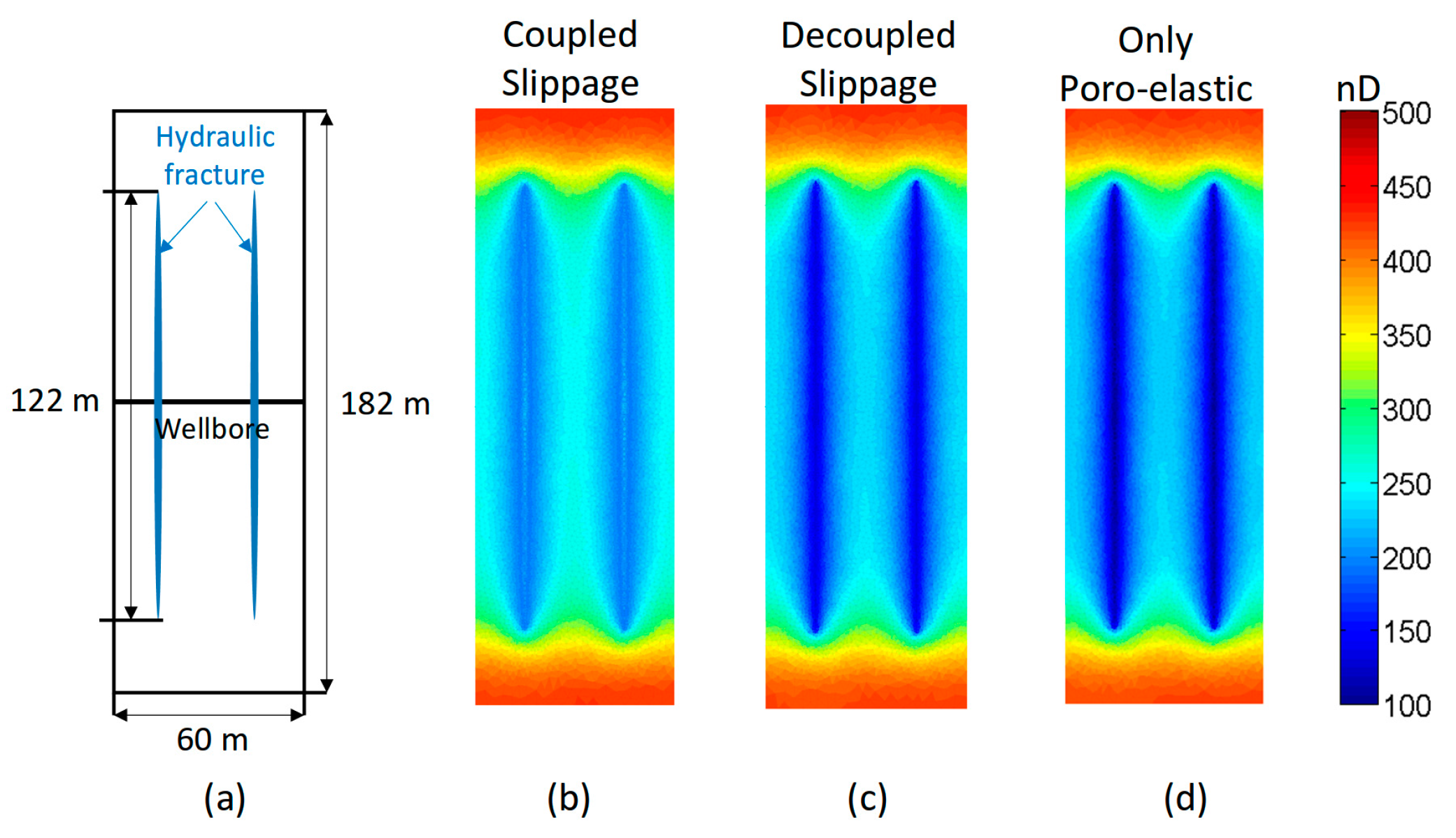
3.1. The Coupled Effect of Poro-Elastic Compaction and Slip Flow

Based on the analysis in Section 3.1, pore volume compaction could result in permeability reduction for Darcy flow. But it will also enhance the gas-slippage effect and lead to a higher apparent permeability when pore pressure is sufficiently low. In this section, we will discuss the coupled effect of poro-elastic compaction and slip flow on the gas well production.

The synthetic reservoir model has a width of 60 m, a length of 182 m, and a height of 50 m. The map view of the model is shown in Figure 4a. Two hydraulic fractures have been stimulated and each has a length of 122 m. According to the work by Gensterblum et al. [12], the range of c_m is from 0.01 MPa⁻¹ to 0.5 MPa⁻¹. Without losing of generality, we selected c_m = 0.08 MPa⁻¹ in this case. The measured pore size ranges from about 20 nm to 200 nm according to several experiments [13,22]. Therefore, the value of 60 nm is used as the pore radius in this case. The rest parameters are taken from Aybar et al. [8], which are based on the typical fluid and rock properties for an unconventional gas reservoir [23,24]. The target depth for this study is set to be 2500 m with the assumption of hydro-static pressure gradient. The confining stress S_hmin is computed using the Eaton’s equation [25]:

$$S_{h\min }=\left(\frac{v}{1-v}\right)\left(S_v-P_p\right)+P_p$$

(17)

where the Poisson’s ratio v is taken as 0.2 according to Eshkalak et al. [23]. The vertical stress S_v is computed using a rock density of 2.3 kg/m³. The confining stress can then be computed as 35.5 MPa for this case. The permeability of the hydraulic fracture is chosen to be 100 D so that the fractures can be considered as infinitely conductive. By doing this, the reservoir performance is dominantly controlled by the matrix properties.

Table 1. Parameter values used in case study.

Parameter	Description	Unit	Value
pinit	initial pressure	MPa	26.9
pw	well pressure	MPa	3.4
hf	fracture height	m	50
μg	gas viscosity	cp	0.02
$k_{d,0}$	initial matrix permeability	nD	500
φm	matrix porosity	-	0.06
v	Poisson’s ratio	-	0.2

summarizes the key parameters used in this work.

Three different scenarios are compared. In the first scenario, we consider the coupled poro-elastic and gas-slippage effect. In the second scenario, we still consider both poro-elastic and gas-slippage effect, but the radius change for slippage flow is ignored. In the third scenario, only the poro-elastic effect is considered. The results are displayed in Figure 5, from which we can observe that the poro-elastic effect is the dominant factor in permeability change. In addition, we can also see that the gas-slippage effect becomes more prominent as pressure depletion continues (higher effective stress). The final permeability for the fully coupled model is much higher than the model that only considers the poro-elastic effect.

Then, we run reservoir simulations for five years for the above three scenarios. At the end of the simulations, the matrix permeabilities corresponding to the three scenarios are shown in Figure 4b–d. Since the lowest fluid pressure appears around the hydraulic fractures, the matrix permeability for the scenario considering the coupled poro-elastic and gas-slippage effect has a local increase. However, for the other two scenarios, the matrix permeabilities are the lowest around the fractures because of the compaction effect.

We then compare the cumulative gas production for the various cases in Figure 6. Another simulation case with constant matrix permeability is performed. We can see that the production profile for the case with constant matrix permeability is distinct from the other three cases (Figure 6). The gas production is consistently higher than the others and it is 23.6% higher than the highest one in the other three cases. For cases with changing matrix permeability, the production performances are very close. As production continues, the gas-slippage effect starts to influence the matrix permeability, which in turn impacts the production, especially for the case with coupled poro-elastic and gas-slippage effect. This is because in this case, the gas-slippage effect is augmented by the reduction in pore size. The gas production for the decoupled model is slightly higher than the case with only the poro-elastic effect.

Finally, we investigate the sensitivity of the poro-elastic coefficient (c_m) and the tube radius on the shale matrix permeability evolution. The ratios of permeability under depletion to the initial permeability (K_m/K_m,0) corresponding to the different parameters are shown in Figure 7. In the first sensitivity test, we vary the poro-elastic coefficient (from 0.06 MPa⁻¹ to 0.1 MPa⁻¹) and keep the other parameters unchanged. According to Equation (14), larger c_m results in more significant permeability decline, which is consistent with the results shown in Figure 7a. One thing worth mentioning is that the case with a larger c_m has smaller pore radius at larger depletion, which leads to stronger permeability enhancement by gas-slippage effect. However, due to the dominant impact of poro-elastic effect, the coupled permeability is still lower than the case with smaller c_m.

In the second test, we vary the initial tube size from 20 nm to 180 nm, and keep the other parameters the same. The results are shown in Figure 7b. It is seen that the case with smaller initial tube radius has larger permeability enhancement, especially at the late stage of depletion (since the gas-slippage effect is more prominent in situations where pore size is small). This observation highlights the necessity of considering the gas slippage in shale because shale has a large amount of micro-scale pores. Note that the coupled poro-elastic and gas-slippage effects are considered for the results in Figure 7.

From the above comparison, we can see that the dominant factor that controls the gas production is the pore volume compaction, though the slippage effect could compensate the production loss slightly. The augmentation of matrix permeability by the micro-scale flow behaviors has been the focus of many researchers in the last decades, but in this study, the results demonstrate that the pore volume compaction effect could be of greater importance.

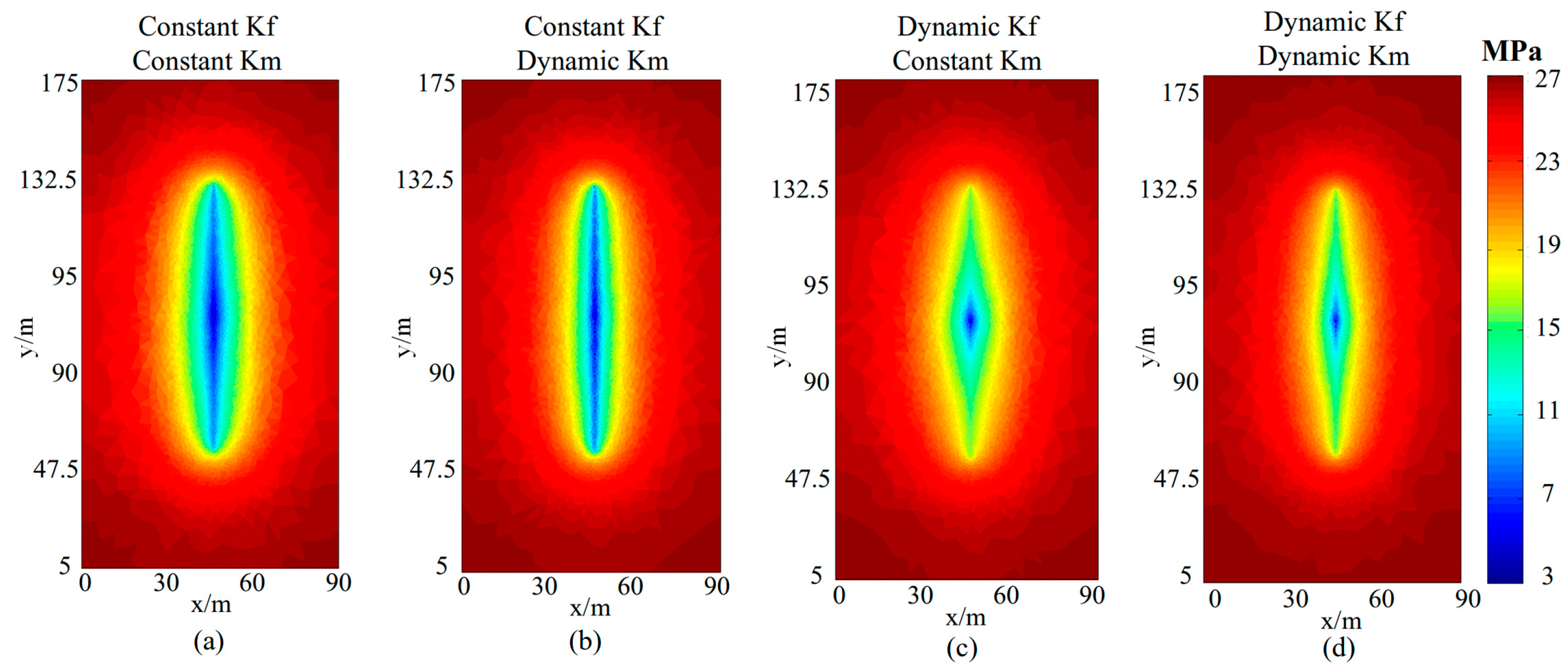
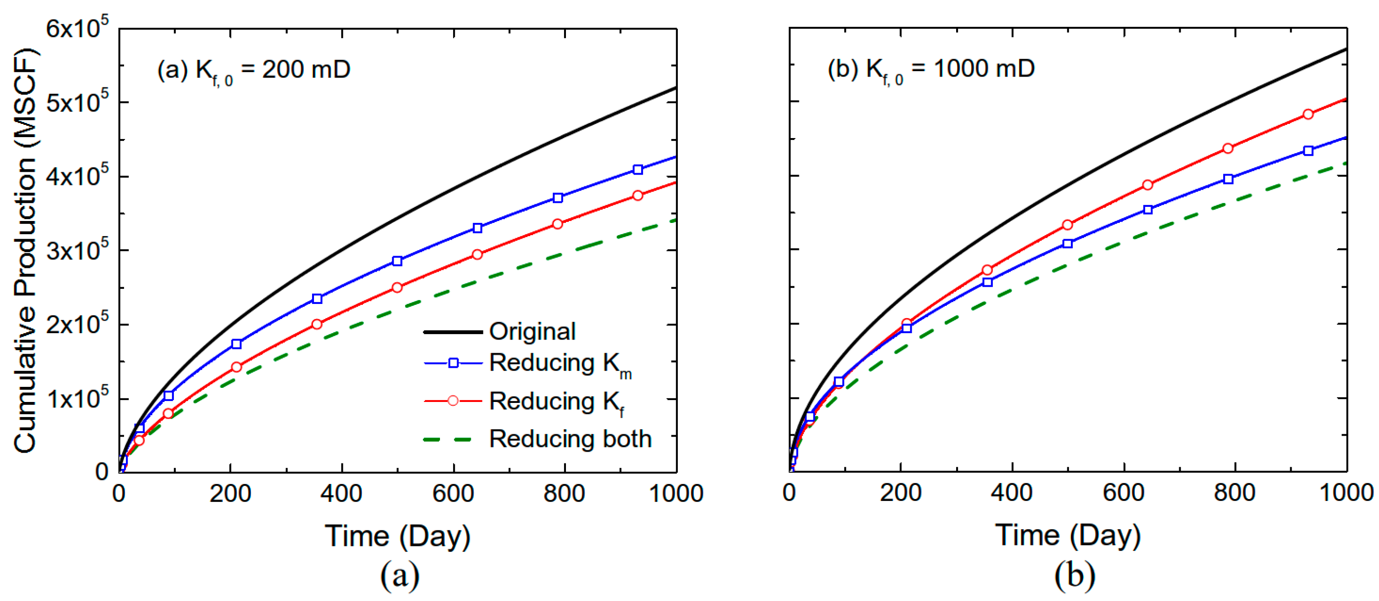
3.2. The Combined Effect of Stress-Dependent Matrix and Fracture Property on Shale Gas Production

We now investigate the combined effect of the stress-dependent matrix and fracture permeabilities on shale gas production. As discussed in Section 3.2, both the fracture permeability and surface area are functions of the effective stress. We first compare the impact of these two effects on shale gas production by fixing the matrix permeability during the simulation. The simulation model is shown in Figure 8a. There are three hydraulic fractures stimulated. The parameters used here are the same as shown in Table 1.

In this model, the relationship between the fracture surface area loss (A_f) and the pressure depletion is modified from Huo and Benson [9] and it is shown as the black curve in Figure 8b. The normalized fracture permeability curve (the ratio of permeability under depletion to initial permeability) is adopted based on the work in Aybar et al. [8] with fracture compliance c_f = 0.1 MPa⁻¹. It is shown as the red curve in Figure 8b.

We consider two different cases. The first case has an initial fracture permeability of 200 mD and the second case has an initial fracture permeability of 1000 mD. The fracture width is 3 mm and is assumed to be constant during the simulation. Again, we run the simulation for five years. The results are shown in log rate–log time plot in Figure 9. The results indicated by “Reducing A_f” are for the case in which only the fracture surface area loss is considered (fracture permeability change is ignored). The results indicated by “Reducing K_f” are for the case in which only the fracture permeability loss is considered. The combined effect of fracture surface area loss and fracture permeability evolution is shown by the green curve. It can be seen that the effect of fracture surface change is only apparent at the very early stage and its impact is much less significant than that of the fracture permeability loss. Note that in the log–log plot, the time starts at 0.1 day, during which significant pressure depletion has already happened. Therefore, the production rates are different at the very beginning of the simulation as shown in Figure 9.

According to the above analysis, we can see that the impact of surface area change is not significant. Therefore, in the following simulations we will ignore this effect and only consider the fracture permeability loss. We now compare the impacts of matrix permeability reduction and fracture permeability reduction on gas production. Again, we consider two cases with 200 mD and 1000 mD initial fracture permeability. We still use the red curve shown in Figure 8b to model the fracture permeability loss. For the matrix poro-elastic effect, we use c_m = 0.08 MPa⁻¹. The simulations are run for five years.

The pressure distributions at the end of the simulation for a group of cases are shown in Figure 10 and Figure 11. Due to the symmetry of the reservoir model (Figure 8), only one third of the reservoir is displayed here. It can be seen that for the case with smaller fracture conductivity (Figure 10) the pressure field is dominantly controlled by the fracture property: cases with the constant fracture property look similar (e.g., Figure 10a,b), while cases with changing fracture permeability look very different (e.g., Figure 10a,c). However, when the fracture is highly conductive (Figure 11), the impact of matrix property becomes more significant. For example, Figure 11d resembles more closely to Figure 11b rather than Figure 11c. This is different from Figure 10.

We then compare the production rates and cumulative production in Figure 12 and Figure 13, respectively. It shows in the early stage that change of fracture permeability has the dominant impact because it happens very quickly. The results with the combined effect resemble closer to the results using only the stress-dependent fracture permeability. As production continues, the impact of matrix permeability reduction becomes significant as the pressure drop within the fracture is gradually stabilized. In this stage, the matrix permeability is the controlling factor that impacts the production performance.

In addition, we see that the relative importance of fracture and matrix permeability reduction also depends on the initial fracture permeability by comparing Figure 13a to Figure 13b. For cases with higher initial fracture permeability, matrix permeability change has a bigger impact. Based on the experimental data, well stimulated hydraulic fractures can easily reach the permeability values greater than 1000 mD. At those circumstances, the stress-dependent matrix permeability is of greater importance to shale gas production.

4. Conclusions

In this work, a coupled model is developed to investigate the impact of matrix and fracture property change on shale gas production. The stress-dependent matrix permeability includes the poro-elastic and the gas-slippage effect. Based on the results obtained from the current work, the following conclusions can be drawn.

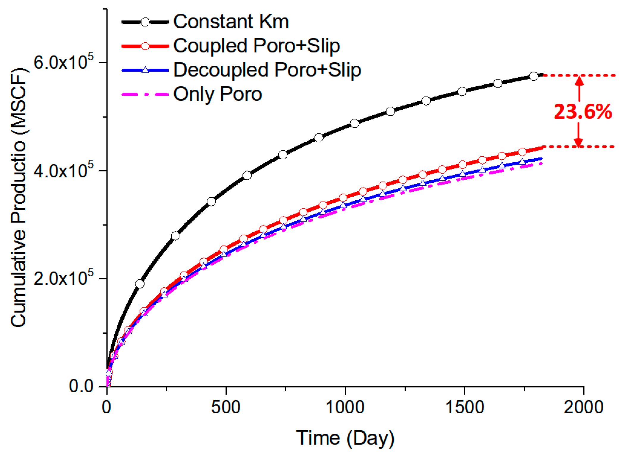
• The coupled poro-elastic and slippage model predicts only slightly higher gas production than the model with only the poro-elastic effect or the model with decoupled poro-elastic and gas slippage-effect. The dominant factor that controls the gas production is still the poro-elastic effect (pore volume compaction).
• Fracture surface area loss was found to affect shale gas production, but the impact is not significant compared with the fracture permeability loss.
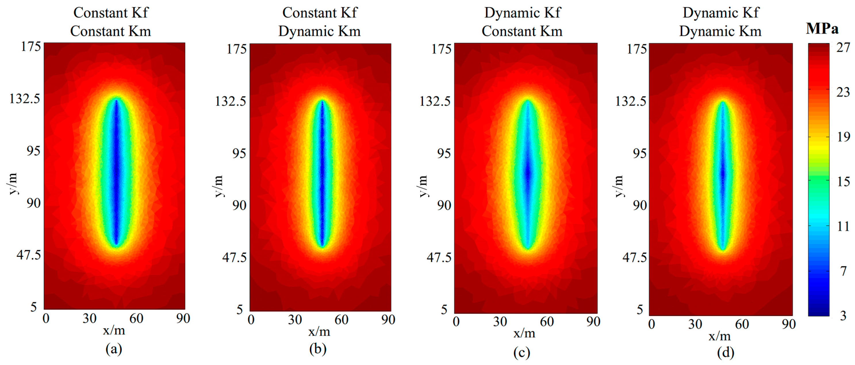
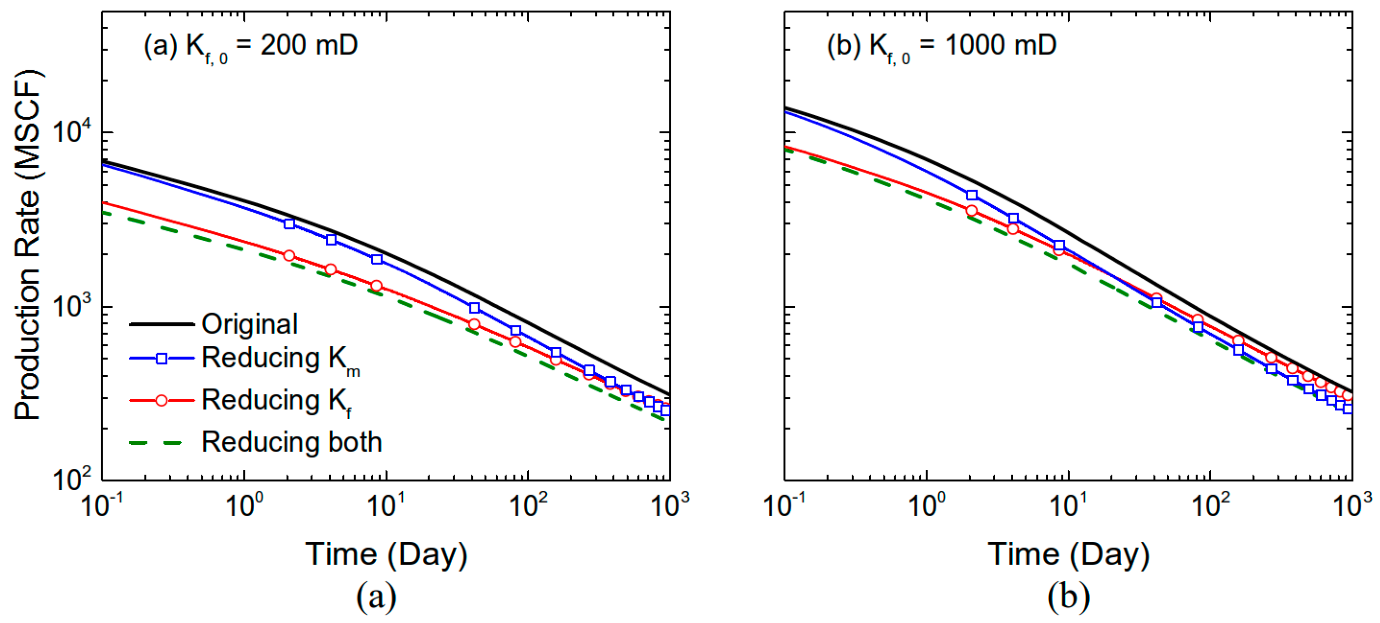
• The impact of stress-dependent fracture property happens at the very early time during the production, while the impact of stress-dependent matrix property is mainly dominated for the longer-term gas production. The matrix permeability evolution can have a significant impact on shale gas production, especially for cases with highly conductive fractures.

References

1. Patzek, T.; Male, F.; Marder, M. A simple model of gas production from hydrofractured horizontal wells in shales. AAPG Bull. 2014, 98, 2507–2529. [Google Scholar] [CrossRef]
2. Valkó, P.P.; Lee, W.J. A better way to forecast production from unconventional gas wells. In Proceedings of the SPE Annual Technical Conference and Exhibition, Florence, Italy, 19–22 September 2010. [Google Scholar]
3. Klinkenberg, L.J. The Permeability of Porous Media to Liquids and Gases; Drilling and Production Practice; American Petroleum Institute: New York, NY, USA, 1941. [Google Scholar]
4. Tanikawa, W.; Shimamoto, T. Klinkenberg effect for gas permeability and its comparison to water permeability for porous sedimentary rocks. Hydrol. Earth Syst. Sci. Discuss. 2006, 3, 1315–1338. [Google Scholar] [CrossRef]
5. Gensterblum, Y.; Ghanizadeh, A.; Krooss, B.M. Gas permeability measurements on Australian subbituminous coals: Fluid dynamic and poroelastic aspects. J. Nat. Gas Sci. Eng. 2014, 19, 202–214. [Google Scholar] [CrossRef]
6. Suarez-Rivera, R.; Burghardt, J. Geomechanics considerations for hydraulic fracture productivity. In Proceedings of the 47th US Rock Mechanics/Geomechanics Symposium, San Francisco, CA, USA, 23–26 June 2013. [Google Scholar]
7. Cho, Y.; Ozkan, E.; Apaydin, O.G. Pressure-dependent natural-fracture permeability in shale and its effect on shale-gas well production. SPE Reserv. Eval. Eng. 2013, 16, 216–228. [Google Scholar] [CrossRef]
8. Aybar, U.; Yu, W.; Eshkalak, M.O.; Sepehrnoori, K.; Patzek, T. Evaluation of production losses from unconventional shale reservoirs. J. Nat. Gas Sci. Eng. 2015, 23, 509–516. [Google Scholar] [CrossRef]
9. Huo, D.; Benson, S.M. An experimental investigation of stress-dependent permeability and permeability hysteresis behavior in rock fractures. In Fluid Dynamics in Complex Fractured-Porous Systems; John Wiley & Sons, Inc.: Hoboken, NJ, USA, 2015; pp. 99–114. [Google Scholar]
10. Pyrak-Nolte, L.J.; Nolte, D.D. Approaching a universal scaling relationship between fracture stiffness and fluid flow. Nat. Commun. 2016, 7, 10663. [Google Scholar] [CrossRef] [PubMed]
11. Ostensen, R.W. The effect of stress-dependent permeability on gas production and well testing. SPE Form. Eval. 1986, 1, 227–235. [Google Scholar] [CrossRef]
12. Gensterblum, Y.; Ghanizadeh, A.; Cuss, R.J.; Amann-Hildenbrand, A.; Krooss, B.M.; Clarkson, C.R.; Harrington, J.F.; Zoback, M.D. Gas transport and storage capacity in shale gas reservoirs–A review. Part A: Transport processes. J. Unconv. Oil Gas Resour. 2015, 12, 87–122. [Google Scholar] [CrossRef]
13. Heller, R.; Vermylen, J.; Zoback, M. Experimental investigation of matrix permeability of gas shales. AAPG Bull. 2014, 98, 975–995. [Google Scholar] [CrossRef]
14. Valkó, P.; Economides, M.J. Hydraulic Fracture Mechanics; Wiley: New York, NY, USA, 1995. [Google Scholar]
15. Ertekin, T.; King, G.A.; Schwerer, F.C. Dynamic gas slippage: A unique dual-mechanism approach to the flow of gas in tight formations. SPE Form. Eval. 1986, 1, 43–52. [Google Scholar] [CrossRef]
16. Tang, G.H.; Tao, W.Q.; He, Y.L. Gas slippage effect on microscale porous flow using the lattice Boltzmann method. Phys. Rev. E 2005, 72, 56301. [Google Scholar] [CrossRef] [PubMed]
17. Zhang, W.M.; Meng, G.; Wei, X. A review on slip models for gas microflows. Microfluid. Nanofluid. 2012, 13, 845–882. [Google Scholar] [CrossRef]
18. Alramahi, B.; Sundberg, M.I. Proppant embedment and conductivity of hydraulic fractures in shales. In Proceedings of the 46th US Rock Mechanics/Geomechanics Symposium, Chicago, IL, USA, 24–27 June 2012. [Google Scholar]
19. Zhang, J.; Ouyang, L.; Zhu, D.; Hill, A.D. Experimental and numerical studies of reduced fracture conductivity due to proppant embedment in the shale reservoir. J. Pet. Sci. Eng. 2015, 130, 37–45. [Google Scholar] [CrossRef]
20. Cao, H. Development of Techniques for General Purpose Simulators. Ph.D. Thesis, Stanford University, Stanford, CA, USA, 2002. [Google Scholar]
21. Zhang, Y.; Gong, B.; Li, J.; Li, H. Discrete fracture modeling of 3D heterogeneous enhanced coalbed methane recovery with prismatic meshing. Energies 2015, 8, 6153–6176. [Google Scholar] [CrossRef]
22. Al Ismail, M.I.; Zoback, M.D. Effects of rock mineralogy and pore structure on extremely low stress-dependent matrix permeability of unconventional shale gas and shale oil samples. R. Soc. Phil. Trans. A 2016, 374, 20150428. [Google Scholar] [CrossRef] [PubMed]
23. Eshkalak, M.O.; Mohaghegh, S.D.; Esmaili, S. Geomechanical properties of unconventional shale reservoirs. J. Pet. Eng. 2014, 2014, 961641. [Google Scholar] [CrossRef]
24. Eshkalak, M.O.; Al-shalabi, E.W.; Sanaei, A.; Aybar, U.; Sepehrnoori, K. Enhanced gas recovery by CO2 sequestration versus re-fracturing treatment in unconventional shale gas reservoirs. In Proceedings of the Abu Dhabi International Petroleum Exhibition and Conference, Abu Dhabi, UAE, 10–13 November 2014. [Google Scholar]
25. Eaton, B.A. Fracture gradient prediction and its application in oilfield operations. J. Pet. Technol. 1969, 21. [Google Scholar] [CrossRef]
Figure 1. Schematic illustrating the effect of pore space compaction.
Energies 10 00996 g001
Figure 2. Schematic showing the pore structures in shale matrix.
Energies 10 00996 g002
Figure 3. Difference between fracture conductivity loss (a) and fracture surface area loss (b).
Energies 10 00996 g003
Figure 4. (a)The schematic of reservoir and fracture configurations; (bd) Matrix permeability for the three scenarios after five years’ production.
Energies 10 00996 g004
Figure 5. Apparent matrix permeability evolution during depletion.
Energies 10 00996 g005
Figure 6. Cumulative gas production for different cases.
Energies 10 00996 g006
Figure 7. The effect of (a) poro-elastic coefficient and (b) initial pore radius on the evolution of matrix permeability during depletion.
Energies 10 00996 g007
Figure 8. (a) Schematic of the model setup and (b) Fracture surface area evolution and fracture conductivity changes during depletion.
Energies 10 00996 g008
Figure 9. Comparison of production rates for initial fracture permeability of (a) 200 mD and (b) 1000 mD.
Energies 10 00996 g009
Figure 10. Pressure distribution after three years of production with an initial fracture permeability of 200 mD. (a) Both fracture and matrix permeabilities are constant during production, (b) only matrix permeability changes during depletion, (c) only fracture permeability changes and (d) both fracture and matrix permeabilities change with production. Km represents matrix permeability, Kf represents fracture permeability.
Energies 10 00996 g010
Figure 11. Pressure distribution after three years of production with an initial fracture permeability of 1000 mD. (a) Both fracture and matrix permeabilities are constant during production, (b) only matrix permeability changes during depletion, (c) only fracture permeability changes and (d) both fracture and matrix permeabilities change with production.
Energies 10 00996 g011
Figure 12. Gas production rates for cases with initial fracture permeabilities of (a) 200 mD and (b) 1000 mD.
Energies 10 00996 g012
Figure 13. Cumulative gas productions for cases with initial fracture permeabilities of (a) 200 mD and (b) 1000 mD.
Energies 10 00996 g013