Article

Offshore Wind Speed Forecasting: The Correlation between Satellite-Observed Monthly Sea Surface Temperature and Wind Speed over the Seas around the Korean Peninsula

New & Renewable Energy Data Center, Korea Institute of Energy Research, 152 Gajeong-ro, Yuseong-gu, Daejeon 34129, Korea
*
Author to whom correspondence should be addressed.
Energies 2017, 10(7), 994; https://doi.org/10.3390/en10070994
Submission received: 4 June 2017 / Revised: 7 July 2017 / Accepted: 11 July 2017 / Published: 14 July 2017
(This article belongs to the Section L: Energy Sources)

Abstract

:
Wind power forecasting is a key role for large-scale wind power penetration on conventional electric power systems by understanding stochastic nature of winds. This paper proposes an empirical statistical model for forecasting monthly offshore wind speeds as a function of remotely sensed sea surface temperatures over the seas around the Korean Peninsula. The model uses the optimal lagged multiple linear regression method, and predictors are characterized by mixed periodicities derived from the autocorrelation between spatially variable satellite-observed sea surface temperatures and wind speeds at all grid points over a period of about ten years (2001 to 2008). Offshore wind speeds were found to be correlated with sea surface temperatures within a seasonal range of two- to four-month lags. In particular, offshore wind speeds were closely associated with the sea surface temperature at lag 4 M, followed by lag 3 M and lag 2 M. Correlation is less at lag 1 M as compared lag 2 M, lag 3 M and lag 4 M. The results demonstrate that this approach successfully produces accurate depictions of monthly wind speeds at the gridded network. The hindcast offshore wind speeds and wind power density showed slightly improved skills compared to the seasonally varying climatology with the value of root-mean square errors, +18% and +23%, respectively. The spatial distributions of the monthly gridded wind speed and wind power density remained fairly stable from one month to another, whereas individual regions displayed slight differences in variability. The results of this study are expected to be useful in establishing guidelines for operating and managing nascent offshore farms around the Korean Peninsula.

1. Introduction

Renewable energy is now recognized as a core means of reducing greenhouse gas emissions. With considerable attention now being paid to the large-scale incorporation of renewable energy into existing energy systems, investments in renewable energy have been expanded around the world [1,2]. In recent years, the Korean government has raised the target goal of renewable energy as a proportion of all energy sources to 20% by 2030 in order to accelerate the reduction of greenhouse gas emissions [3]. Among all energy sources, the national offshore wind power capacity is estimated to reach 12 GW by 2030 in Korea, which accounts for half of all renewable energy sources and 10% of the total power generated by the installed power generators. However, the uncertainty of power systems increases with an increase in electricity production resulting from variable renewable energy sources when large-scale (10% or higher) wind power generation is added to the existing power generation systems due to the aggressive government policy [4,5,6,7]. Advanced countries whose electricity production consists of over 10% wind energy, such as Denmark and Germany [8], are already operating their own intelligent power systems with wind power forecasting for transmission system operators in maintaining the reliability and stability of the electricity supply. In the case of Korea, the Korea power exchange (KPX) is responsible for planning fuel procurement, scheduling the maintenance of power generation facilities, and assessing the energy trade and sales in order to limit the risks and maximize profits [9]. This is an operational mode of power generation that takes demand into account. Nonetheless, a forecasting technology that considers renewable energy, the supply of which can fluctuate massively, has yet to be included. Thus, operational wind power forecasting according to natural variations is necessary in order to increase the penetration of wind power generation and reduce the base-load generator in time.
Wind speed and power forecasting has various time horizons, such as very short-term perspective (from a few seconds to 30 min ahead), short-term (from 30 min to 6 h ahead), medium-term (from 6 h to 1 day ahead), and long-term (from 1 day to 1 week or more ahead) forecasting [10,11,12]. The time scale for the integration of wind power into the existing energy system needs to consider that for the power operating system [2]. The time scales used in the KPX operating load-forecasting model are daily, monthly, and annual. In particular, the forecasting technology for wind power’s peak electricity demand is important for capacity planning and maintenance scheduling not only in the daily short-term but also the long-term forecasting horizon (i.e., more than one month). On the other hand, offshore rather than onshore wind power has been increasing because of land regulations and saturation effects [13]. Offshore wind power requires longer maintenance and repair time and higher costs compared to onshore wind power. The Korean government promised to build up the capacity of offshore wind power plants to 2.5 GW in the West-South Sea region [14,15]. Most of the upcoming wind power installation projects would cover offshore wind farms. Although a number of offshore wind farm projects are under way, however, no systematic studies on offshore wind forecasting around the Korean Peninsula have been conducted, and no guidance on forecasting performance for technical development has been provided. Therefore, monthly offshore wind power forecasting is urgently needed in Korea considering the continuous construction plans for offshore wind power.
In fact, one of the most important problems in wind power forecasting is that of expanding the forecasting horizon. In general, wind power forecasting considers a shorter time scale than the monthly-basis scales. Such a short-term forecasting method was improved dramatically after a large number of studies were conducted in nations with highly developed wind power sources and a high penetration of wind energy in the electrical grid. It should be noted that long-term forecasting of more than one week has not been used even in the aforementioned nations due to the physical gap in weather and climate systems. Kritharas and Watson [16], and Azad et al. [17] attempted monthly wind speed forecasting based on an analysis of long-term time-series patterns over the past few decades using the autoregressive method and artificial neural networks, respectively. Nonetheless, such studies were limited to investigating on-land wind in several regions only; no results of studies on offshore monthly wind forecasting have been included. Recently, new projects such as Ukko or EUPORIA in Europe have gotten under way due to demands from the energy markets [18,19]. These projects in the European Union (EU) have used dynamic climate simulations to produce long-term forecasting data in order to reduce quarterly and annual energy prices, and are generally focused on expanding the forecast horizon to enable seasonal wind forecasting. It is to be noted that Europe and Korea have fundamentally different weather systems, as well as electricity production portfolios that deviate significantly in terms of the time scale. Thus, the previous study results are not as suitable for use as they are.
In this study, a monthly wind speed forecasting model for forecasting wind power was constructed and evaluated. Monthly wind speeds were hindcast statistically using remotely sensed sea surface temperatures, according to a new approach. The Korean Peninsula is located in the monsoon climate zone and surrounded by seas on three sides, as shown in Figure 1. This indicates that adjacent seas would have various climatic characteristics locally [20]. The long-term features of offshore wind in the seas around Korea should be compared and analyzed to identify climatological patterns, but reliable wind measurements throughout these waters are lacking. The offshore wind data extracted from satellites in recent years have been utilized successfully to investigate the evaluation of offshore wind power [21,22]. In particular, Oh et al. [22] analyzed remote sensing offshore wind that was spatially uniform and discovered that wind power resources were rich in the southwest coast, southern coast, and southeast sea regions of the Korean Peninsula. Nonetheless, their study only sought to evaluate resources in order to select optimal places for wind power. Remotely sensed observations were used to perform accurate offshore wind forecasting over a wide range of areas as potential sites. In particular, the sea surface temperature is known to be a representative variable that assists understanding of air-sea physics. We employed it as a predictor in the statistical wind-forecasting model. In addition, most statistical models based on long-term data analysis have been limited to an analysis of specific areas, followed by predictions of power generation facilities at specific points. By contrast, this study has attempted to perform grid-based wind speed forecasting that enables flexible forecasting by size according to the new designs of offshore wind farms. The rest of this paper is organized as follows: Section 2 describes the data used; Section 3 discusses the procedure for establishing the statistical model and its evaluation; Section 4 presents the results of the experiments; and, finally, Section 5 presents the summary and the conclusion.

2. Data

To construct and evaluate an offshore wind speed forecasting model as a function of sea surface temperature, remotely sensed surface observations—such as sea surface temperature and offshore wind speed—were utilized in this study. Satellite data were collected to overcome the limitations of the space range offshore where measurement data were hard to acquire. The seas surrounding Korea are divided into the Yellow Sea, East Sea, and South Sea according to their geospatial locations as shown in Figure 1. Each sea has a significantly different bathymetry (depth in meters). The depth of the Yellow Sea is mostly less than 80 m, whereas that of the South Sea is less than 80 m near the coast and around 200 m offshore. The East Sea has an average depth of 1700 meters, although it can be as deep as 5000 meters in places, which makes it a deep sea. Thus, most areas of the Yellow Sea and South Sea are 80 meters deep near the coast, except for the deep-sea area of the East Sea. This means that the characteristics of wind conditions differ regionally due to the air-sea climate interaction. Thus, spatially variable sea surface temperatures and winds were used for ten years because they were typical thermal and dynamical variables in the surface between the sea and the atmosphere.

2.1. Sea Surface Temperature Data

This study used satellite-observed sea surface temperature for estimating changes in wind speed because temperature is one of the principal climate factors and satellite-observed sea surface temperature is able to estimate variations in winds, swells, and waves [23,24]. The sea surface temperatures are the optimum interpolation sea surface temperatures (OISST), as re-analysis data based on ships, buoys, and advanced, very high-resolution radiometer in satellites [25]. The OISST data cover the world, and use a horizontal resolution composed of 25 km grid spacing. Here, one degree of monthly OISST, ranging from December 1999 to November 2011, was taken from the National Center of Environmental Prediction (NCEP). The long-term OISST data are known to match with in situ data with warm biases and 1 °C of the root mean square error in the study areas [26,27].

2.2. Wind Speed Data
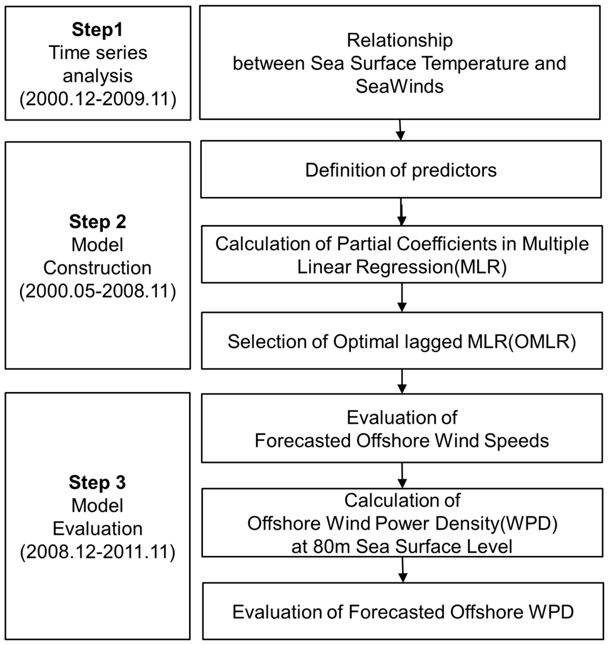
Two sea winds were observed from the Quick Scatterometer (QSCAT, [28]) and the Cross-Calibrated Multi-Platform (CCMP, [29]). These satellite winds were used to investigate the relationship with the sea surface temperature and to evaluate the wind and power forecasting model. These are data blended spatially with the NCEP reanalysis data. QSCAT was launched in June 1999 by the National Aeronautics and Space Administration and operated in the Ku band until November 2009 [30]. 10 m wind speeds were estimated from the correlation with backscattered power. QSCAT has an 1800 km-wide range and maps the global oceans twice a day. The monthly QSCAT data utilized in the analysis are latitude-longitude grid data with 0.5-degree resolution taken from December 1999 to November 2009. The CCMP data sets refer to the cross-calibrated satellite winds of information derived from the Special Sensor Microwave Imager (SSMI/I), the Special Sensor Microwave Imager Sounder (SSMIS), the Advanced Microwave Scanning Radiometer-Earth Observing System (AMSR-E), the Tropical Rainfall Measuring Mission (TRMM), the TRMM Microwave Imager (TMI), QSCAT, WindSat, and other satellite equipment. Additional CCMP data were collected from December 2009 to November 2011 without the QSCAT data used with 0.25-degree grid resolution.

3. Method

The statistical monthly wind speed forecasting model proposed in this study employed the multiple regression method by considering the correlation between sea surface temperature and offshore wind speed. As shown in Figure 1, all of the seas except for the deep-sea region of the East Sea were advantageous to offshore wind power, so the study areas targeted them all [31]. The target area ranged from 120.5° E to 135.5° E in the east-west direction and from 30.5° N to 44.5° N in the south-north direction.
The schematic diagram of wind speed forecasting is shown in Figure 2. The process of constructing the model was largely divided into three phases: time-series analysis, model construction, and model evaluation. The analyzed data and the period for each phase were slightly different. Time-series analysis was conducted on the period from December 1999 to November 2009, which is the longest record of QSCAT wind speeds. Afterward, the model was developed using the data from May 2000 to November 2008. This period is the so-called training or fitting period, which is used in the development of the forecasting model-based on the empirical statistical method. Finally, the model was evaluated for the remaining period from December 2008 to November 2011.

3.1. Time Series Analysis

The wind speed forecasting has been done utilizing the multiple linear regression (MLR) method. Multivariate analysis is done using long-term OISST time series through autocorrelation analyses of QSCAT wind speeds. Step 1 in Figure 2 was basically conducted to identify the relationship between the two variables. The monthly OISST and QSCAT wind speeds were utilized after analyzing normality and periodicity, respectively, over the study period [32], after which spatio-temporal monthly and seasonal variabilities were compared using time lag analysis. Here, the data were normalized to compare the different units and ranges of the OISST and QSCAT wind speeds on the same scale.

3.2. Statistical Model for Wind Speed Forecasting

The wind speed forecasting model utilized the following MLR equation, assuming the error term to be 0 due to the accidental effect:
Y ( i , j , t ) = α ( i , j , t ) + lag β ( i , j , t lag ) × X ( i , j , t lag )
where the predictor, X refers to the OISST and predictand, Y refers to the predicted monthly wind speeds; α and β indicate the regression constant and coefficients of the predictor variables, respectively; i , j and t denote the target grid of longitude and latitude and the time of prediction, respectively; and lag represents the time delay operator.
The most significant characteristic of the model is the use of mixed periodicity for the OISSTs that are highly correlated with the QSCAT wind speeds as independent variables. Mixed periodicity refers to the lags composites [33]. First of all, the autocorrelation was analyzed to identify the proper lags of mixed periodicity between two variables in time. In the results, 0.4 was set as the criteria for the correlation between the measured wind speed and the forecast wind speed; while a lag that exceeded the criteria was regarded as a proper lag. α and β were then calculated by comparing the predicted and observed wind speeds for the fitting period. Then, a number of model equations were constructed using the calculated coefficient and predictor. Among these potential models, a wind speed forecasting model with good performance was selected based on statistically significant values such as the root-mean-square error (RMSE), the slope of the line of best fit (SLOPE), and the correlation coefficient (CORR). The significance was judged to be a 95% confidence level based on the t-test. The optimal lag that showed the best performance (i.e., the RMSE is close to zero, and the SLOPE and CORR are close to one) in the basic statistics was selected, and the optimal lagged multiple linear regression-based wind speed forecasting model (OMLR) was determined accordingly.

3.3. Model Evaluation

The proposed OMLR model was evaluated for the evaluation period. To evaluate the performance of the predictability of the constructed wind speed forecasting model based on mixed periodicity, the cyclically varying monthly model was utilized as seasonally varying climatology during this study period. The study is in fact influenced by strong seasonal variations as shown in Section 4.1. Monthly varying wind speed and power predictability in the model were evaluated based on a spatio-temporal comparison and the quantitative error statistics of the RMSE and the normalized RMSE (nRMSE). Next, theoretical wind power forecasting was evaluated by adding the calculation of wind power density (WPD). The wind speed at 80 m above sea level (asl) as the typical height of a wind turbine was extrapolated by the following power-law equation, with the satellite-retrieved wind speeds at 10 m asl [21]:
V z = V z r ( z z r ) α
where z and z r represent the height and reference height above sea level, respectively; and V z and V z r denote the wind speed at heights z and z r , respectively. For the wind shear exponent, α the value of 0.097 to 0.0147 is used in the sea, which is measured by met mask tower over the study sea [34]. The wind energy density is calculated by Equation (3):
P = 1 2 ρ V 3
where ρ is the air density (1.225 kg/m3). In particular, the WPD was divided into seven classes and verified to check the wind power applicability of the forecasting model [35,36].

4. Results and Discussion

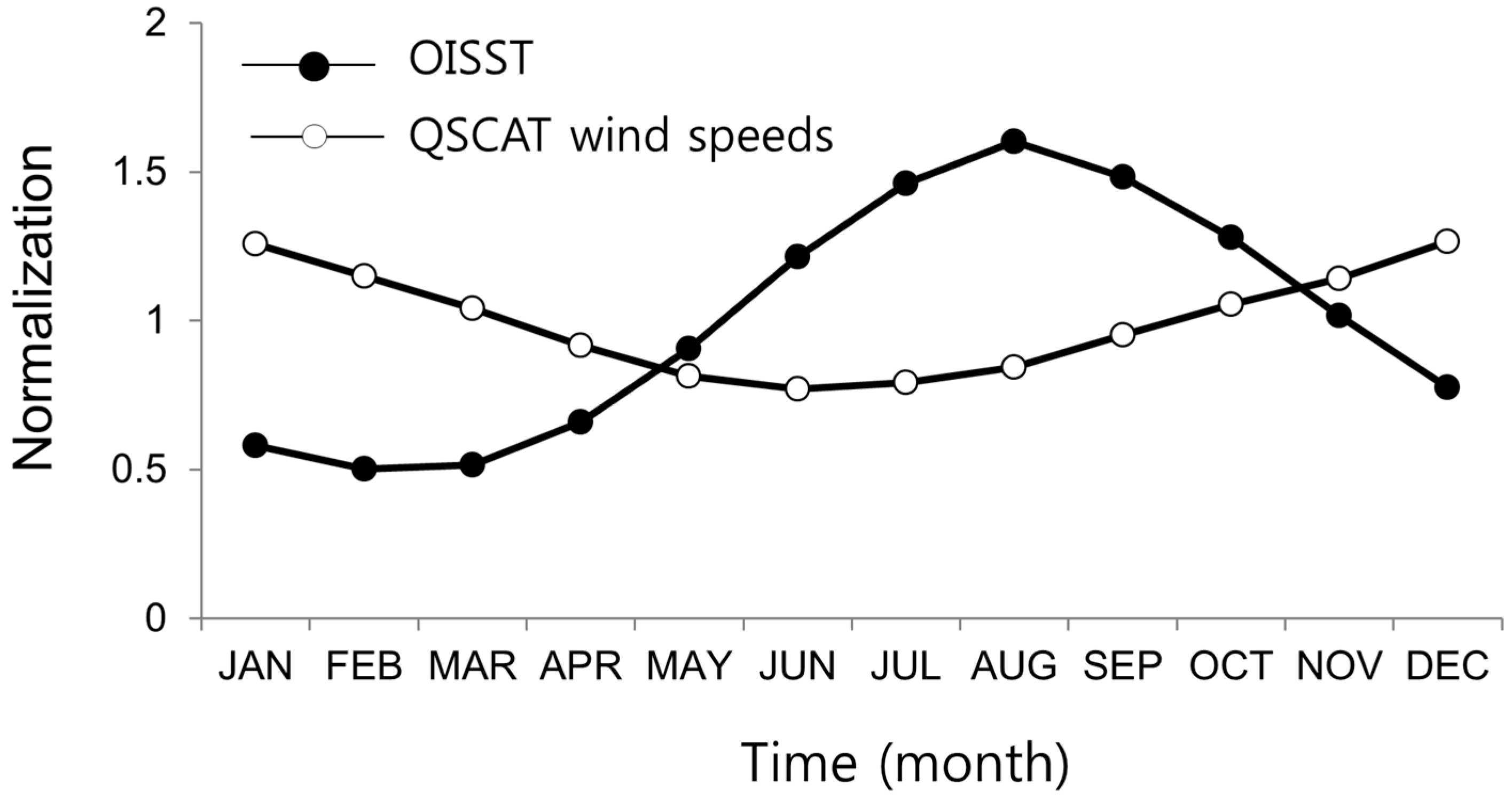
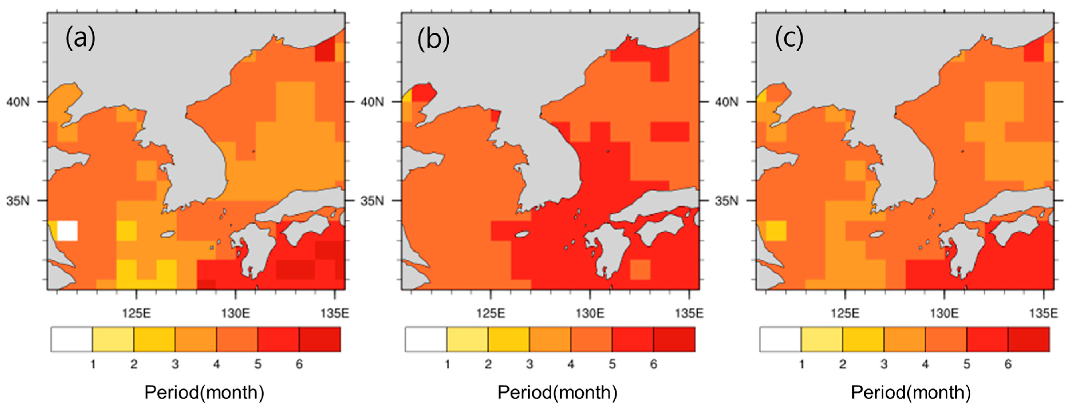
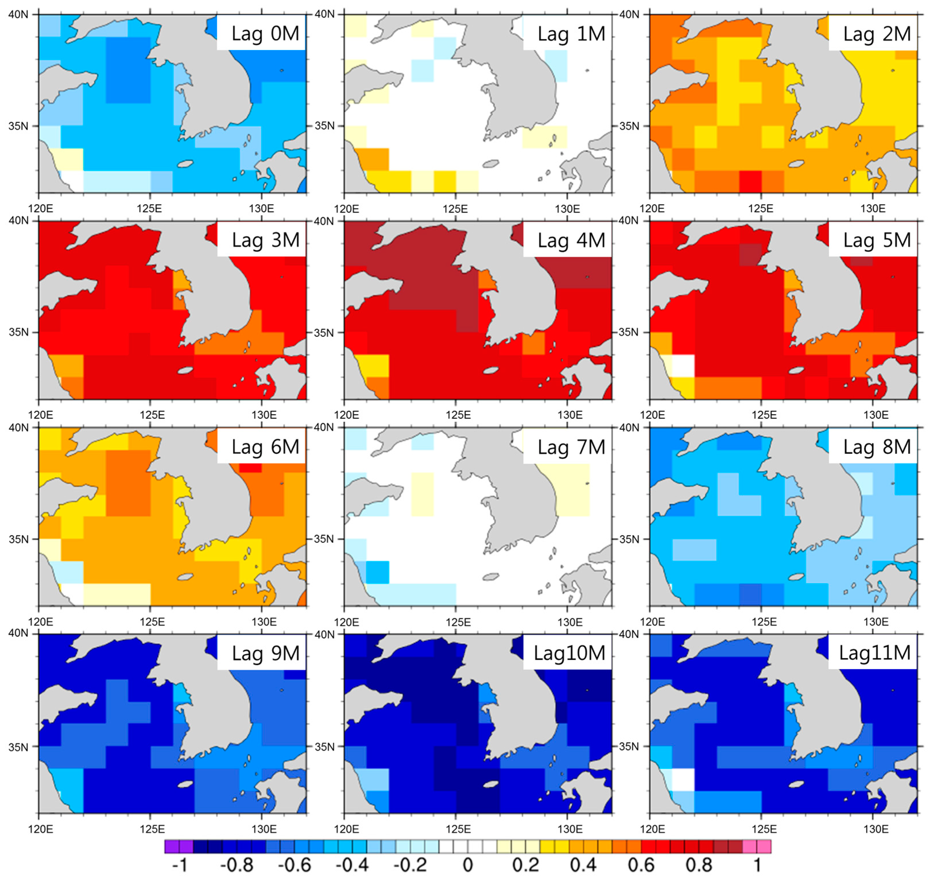
4.1. Relationship between Monthly Sea Surface Temperature and Wind Speed

In this section, the spatio-temporal relationship between the predictor and the dependent variables, which are required to construct a statistical wind speed forecasting model, was analyzed. Figure 3 shows the monthly variability of the spatial averaged OISST and QSCAT wind speeds for the time-series analysis period. The OISST and QSCAT wind speeds showed a negative correlation. This result is known to be a common feature caused by the air-sea interaction in the mid-latitude [36]. A strong QSCAT wind occurred at a speed of 8.81 m/s from December to January (winter). During the period from May to August (summer), the wind speed weakened to 4.91 m/s. On the other hand, the OISST was 8.93 °C and 24.80 °C in February and August, respectively, which were the lowest and highest values recorded during the year. These seasonal variations were also represented in the power spectrum, as shown in Figure 4. The OISST and QSCAT wind speeds showed nearly the same dominant periodicity, reaching a peak in three months. Note that there were some out-of-phase delays between the monthly OISST and QSCAT wind speeds.
To investigate the out-of-phase time delay between two variables, the lags for the two peaks in the seasons were spatially analyzed, as shown in Figure 5. Figure 5a,b represents the distributions of the time lags between the summer OISST and the winter QSCAT wind speeds (the highest SST-WS), and between the winter OISST and the summer QSCAT wind speeds (the lowest SST-WS), respectively, over the seas observed in the study. For the highest peaks, three- and four-month time lags were revealed in the southern and northern seas, whereas the lags between the lowest peaks were four to five months in the northern and southern seas. This means that the wind speeds became slower after four to five months ahead of the SST (sea surface temperatures) dropped in region for the lowest peaks. The seasonal time lags also varied over the South Sea, whereas those were constant with the four-month lags over the Yellow and Northeast Seas. In relation to the synoptic flow, the seasonally constant time-lagged area of the northeast sea is likely to be related to airflow circulation during the monsoon season. On the other hand, the seasonally different time-lagged area of the South Sea was deemed to be affected by the Kuroshio Current [26] as the OISST cooled late along the strong Kuroshio Current, where the change in wind speed was small. The annual mean of the two seasonal lags did not show a large regional difference, but regionally different lags remained (Figure 5c). This indicates that the offshore wind speed model should be established on the sub-basin and intra/inter-seasonal scale in order to consider the different spatio-temporal features between sea surface temperatures and wind speeds in the seasons and regions. Thus, since this study sought to predict the variability of monthly wind speed and power rather than the annual mean wind speed, the mixed periodicity of multiple months at all grid points is introduced in the next section to reflect the monthly variability as much as possible.

4.2. Construction of a Monthly Wind Speed Forecasting Model
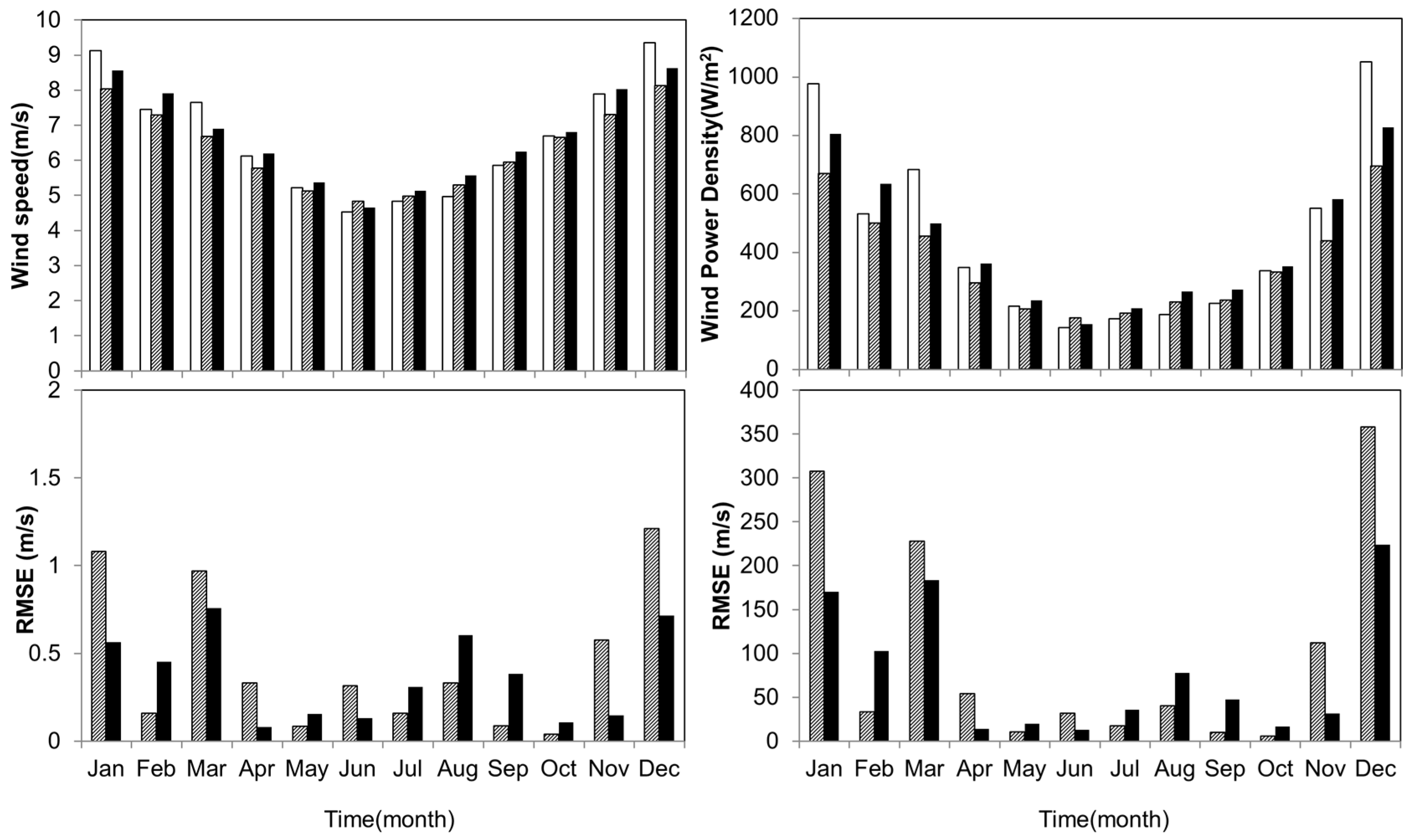
In order to establish a wind speed forecasting model as a function of the mixed periodicities of sea surface temperature, proper mixed periodicities were extracted based on the autocorrelation of the OISST and QSCAT wind speeds during the fitting period. Here, monthly sea surface temperatures corresponding to time lags become predictors in the MLR equation. Figure 6 shows the spatial patterns of the autocorrelation coefficient (CC) with regard to the OISST and QSCAT wind speeds. Time lags with CC values of over 0.6 were three to five months or nine to eleven months. The forecast lead times of the OISST, which can estimate the wind speeds, ranged from one to six months, showing positive CCs. The CC for the one-month lead time (lag 1 M in Figure 6) varied in the range of −0.2 to 0.2, wherein the OISST was not correlated with the wind speed. The OISST at two- and six-month lead time (lags 2 M and 6 M in Figure 6) showed CCs with normal values of 0.3 to 0.4. Although relatively low CCs (0.2–0.4) were observed in a part of the Yellow Sea near the coast of the Korean Peninsula, the OISST at three- to five-month lead time (lag 3 M to 5 M in Figure 6) revealed high CCs with wind speeds of 0.6 or higher over most of the study area. Thus, proper lags were within a range of two- to six-month lead time, whose correlation was 0.4 or higher, and the OISST in those time lags was applied as the predictor in potential wind speed forecasting models.
Table 1 presents the performance of potential wind speed forecasting models for the part of the evaluation period where QSCAT is available. A total of 15 potential models were constructed with strong correlations between the independent and dependent variables. Various model equations were compared according to the lag-windows of mixed periodicity. Each of the statistics was calculated in units of mixed periodicity, with the column and row indicating the starting and ending lag-windows, respectively. The mean range of the RMSE and the CORR in the models with relatively good performance of 1.5 m/s or lower RMSE and 0.8 or higher CORR was 1.12 ± 0.28 m/s and 0.83 ± 0.02, respectively. The multiple regression model of mixed periodicity showed better performance than the simple regression model of single periodicity. In general, as the width of the lag-windows increased, the models’ performance tended to improve with reduced RMSEs and SLOPEs and increased CORRs, with values of up to 0.69, 0.87, and 0.86, respectively. Lag-windows composed with two- to four-month lead time showed statistically significant increased performance, whereas lag-windows with five- to six-month lead time for the performance of potential models were similar, showing no significant differences with the RMSE and CORR values of 0.2 m/s and 0.05, respectively. Lag-windows composed with four- to six-month lead time showed goodness of fit (i.e., a 1.5 m/s or higher RMSE and a 0.8 or lower CORR). The SLOPE was reduced by up to 0.85 when the time lag was extended to five- or six-month lead time, showing a deviation from the line of the best fit in some cases. The model with lag-windows from two- to four-month lead time was selected as the OMLR focusing on a SLOPE close to 1, because this model assumes linearity between the predictor and the predictand.
The contribution of the multivariate predictors in the OMLR was compared. The spatially averaged partial correlation coefficient of β 1 (CC of sea surface temperature at two-month lead time), β 2 (CC of sea surface temperature at three-month lead time), β 3 (CC of sea surface temperature at four-month lead time) were 0.15, −0.17, and 0.21, respectively. The variable that showed the maximum CC was the SST at four months ago. In addition the statistical model for forecasting monthly wind speed utilized the latest wind speed and examined for climate indices as an additional predictor in this model. Climate factors (i.e., Artic Oscillation, Southern Oscillation index, Multivariate ENSO index to monitor El Niño/Southern Oscillation (ENSO)) highly affected on seasonal variations over East Asia centering the Korean Peninsula were investigated in order to consider variability in wind speeds. It was observed that there were no significant effects on monthly wind speeds during the study period, although Artic Oscillation correlated with one month ahead.

4.3. Evaluation

The proposed OMLR was evaluated in terms of not only wind speed but also WPD by satellite observations and a seasonally varying climatology for the model evaluation period. In particular, WPD was applied to investigate the use of the OMLR for wind power forecasting. The persistence model has been used frequently to compare the statistical model as a reference in previous studies. Figure 7 shows the monthly variability of the spatially averaged wind speeds and the WPD over the study area. The monthly wind speeds estimated by the climatology and the OMLR expressed the monthly variability of the measured wind speeds well. The slowest and strongest wind speeds were observed in June and December. Moreover, the climatology and the OMLR underestimated the wind speeds by 66% and 25%, of the months of the total years, particularly for winter seasons. RMSE values were 0.45 m/s and 0.37 m/s for the climatology and the OMLR, respectively. The OMLR showed better performance during winter seasons, when the wind speed is pronounced. The monthly variations in the WPD were large compared with those of the wind speed at 10 m asl. When this was compared with that of the WPD at 80 m asl, the RMSE even exceeded 150 W/m2 in some cases. The WPD taken from the OMLR showed a relatively smaller RMSE than that taken from the climatology. The OMLR revealed up to 137.56 W/m2 RMSE compensation compared to that in the climatology, implying that about two grade differences can result according to the WPD. Overall, the OMLR exhibited a better predictive performance than the climatology.
In order to validate the performance for the model for forecasting spatio-temporal offshore wind power, the spatially variable WPD was also compared. Figure 8 illustrates the spatial distribution of monthly variability in terms of WPD grade. The observed WPD grades in most of the regions were higher than Grade 3 (250–375 W/m2), except from June to July. In the summer season (June to August), while WPD grades lower than Grade 3 were noted throughout the regions. WPD grades higher than Grade 3 were pronounced in the winter season (November to March) over most of the regions. Although the hindcast WPD grades were somewhat overestimated in the regions and months, the spatial characteristics of the WPD grades between the OMLR and the observation were quite similar.

5. Conclusions

This study developed a model for forecasting monthly offshore wind speed as a function of sea surface temperature with regard to the nearby seas around the Korean Peninsula, where an offshore wind power project is actively under way. Based on the correlation between wind speed and sea surface temperature measured by satellite over a long period of time from 2000 to 2008, a grid-based multi-regression statistical model was proposed to predict wind speed and wind power density.
The satellite wind speed showed a strong negative correlation with time lag to the sea surface temperature. Seasonal wind speeds that were high in winter and low in summer had an approximately four-month time lag to the seasonal sea surface temperature, which was high in summer and low in winter in the West and East Seas, while a three- to five-month lead time was revealed in the South East Sea. Specifically, monthly wind speeds were highly correlated with the two- to six-month lead times of the sea surface temperature regionally. These lag correlations between the two variables were employed as a predictor in the wind speed forecasting statistical model based on the multiple linear regression method, which showing that the optimal lag window was two- to four-month lead time, which was statistically significant. Among these lags, the largest contribution was the four-month lead time. Sea surface temperatures at four-month lead time can explain the wind speed with much more contribution than those of the three- and two-month lead time in sea surface temperature. The results of the evaluation of the predictability of wind speed and the applications to wind power densities in the forecasting model revealed good performance (RMSE 0.37 m/s, CORR 0.81). Despite some tendency toward a slight overestimation or underestimation of wind speed in summer and winter, the seasonal variance of the predicted wind speed was similar to that of the actual wind speed. Compared to the seasonally varying climatology, the developed model showed RMSE that was smaller by 0.08 m/s and CORR that was larger by 0.3. Furthermore, the seasonal variance was well expressed with the same prediction characteristics as those of wind speed when it was evaluated for the wind power grade according to the wind power density at 80 m asl.
The results of this study confirmed that monthly mean offshore wind speeds can be estimated using sea surface temperatures two- to four-months in advance over the seas around the Korean Peninsula. This was due to the general negative correlation between wind speed and sea surface temperature in the mid-latitude derived through monthly analysis, which indicates that a change in wind speed in the strong monsoon zone can be explained by a change in sea surface temperature in one seasonal period. Furthermore, the wind speed and power forecasting model of the multiple regression model using high-frequency periodicity showed RMSE that was smaller by 0.08 m/s on average than that of the climatology. It was also found that a 17.59% change in wind speed at 10 m above sea level can reduce the RMSE of the wind power grade at 80 m above sea level by 22.25% on average. This indicates that, within a wind energy system, accurate forecasting of wind speed from the optimal lagged multivariate regression model would help to minimize scheduling errors and in turn increase the reliability of the management and operation of electric power. Finally, the wind speed and power forecasting statistical model, on which mixed periods of individual weight for each grid were reflected, had the advantage not only of being able to predict offshore wind power at a specific location, but also of possible conversion of utilization range that could be applied to power operation systems in accordance with the designs in the offshore wind farms. However, the change in wind speeds are influenced by various factors associated with wind regimes over the Korea Peninsula [23]. This model needs to be optimized further by considering ocean-forced global phenomena to elaborate spatially varying periodicity further for the extended study period. Although predictability should be also improved by adding predictor analysis on a more detailed time scale and horizontal resolutions than one degree so as to ensure better predictability of monthly wind speed than the current model. The main result of this study is an offshore wind speed and wind power forecasting technology of an appropriate level that must be secured in preparation for the adoption and operation of new offshore wind power generators in addition to existing power operation systems in the future. Thus, the results of this study are expected to be utilized in related studies

Acknowledgments

This work was conducted under the framework of research and development program of the Korea Institute of Energy Research (B7-2434).

Author Contributions

Jin-Young Kim and Hyun-Goo Kim conceived and designed the experiments; Jin-Young Kim performed the experiments; Jin-Young Kim, Hyun-Goo Kim, and Yong-Heack Kang analyzed the data; Jin-Young Kim and Hyun-Goo Kim contributed reagents/materials/analysis tools; Jin-Young Kim wrote the paper.

Conflicts of Interest

The authors declare no conflict of interest.

References

  1. Lund, H. Large-scale integration of wind power into different energy systems. Energy 2004, 30, 2402–2412. [Google Scholar] [CrossRef]
  2. Strbac, G.; Shakoor, A.; Black, M.; Pudjianto, D.; Bopp, T. Impact of wind generation on the operation and development of the UK electricity systems. Electr. Power Syst. Res. 2007, 77, 1214–1227. [Google Scholar] [CrossRef]
  3. The Korea Herald. Available online: http://www.koreaherald.com/view.php?ud=20170510000794 (accessed on 10 May 2017).
  4. Energy Efficiency & Renewable Energy. Available online: https://apps2.eere.energy.gov/wind/windexchange/filter_detail.asp?itemid=1456 (accessed on 19 January 2007).
  5. Resende, F.O.; Peças Lopes, J.A. Management and control systems for large scale integration of renewable energy sources into the electrical networks. In Proceedings of the EUROCON—International Conference on Computer as a Tool, Lisbon, Portugal, 27–29 April 2011. [Google Scholar] [CrossRef]
  6. Stoutenburg, E.D.; Jenkins, N.; Jacobson, M.Z. Variability and uncertainty of wind power in the California electric power system. Wind Energy 2014, 17, 1411–1424. [Google Scholar] [CrossRef]
  7. Krishnappa, H. Long-term minute-wise wind forecasting using time series modelling. Int. J. Serv. Sci. Technol. 2016, 9, 179–188. [Google Scholar] [CrossRef]
  8. Klaassen, G.; Miketa, A.; Larsen, K.; Sundqvist, T. The impact of R & D on innovation for wind energy in Denmark, Germany and the United Kingdom. Ecol. Econ. 2005, 54, 227–240. [Google Scholar] [CrossRef]
  9. Phuangpornpitak, N.; Prommee, W. A study of load demand forecasting model in electric power system operating and planning. GMSARN Int. J. 2016, 10, 19–24. [Google Scholar]
  10. Soman, S.S.; Zareipour, H.; Malik, O.; Mandal, P. A review of wind power and wind speed forecasting methods with different time horizons. In Proceedings of the North American Power Symposium, Arlington, TX, USA, 26–28 September 2010. [Google Scholar] [CrossRef]
  11. Singh, S.; Kumar, N. Wind power forecasting: A survey. Int. J. Eng. Res. Gen. Sci. 2016, 4, 802–806. [Google Scholar] [CrossRef]
  12. Fortuna, L.; Nunnari, G.; Nunnari, S. A new fine-grained classification strategy for solar daily radiation patterns. Pattern Recogn. Lett. 2016, 81, 110–117. [Google Scholar] [CrossRef]
  13. Markard, J.; Petersen, R. The offshore trend: Structural changes in the wind power sector. Energy Policy 2009, 37, 3545–3556. [Google Scholar] [CrossRef]
  14. Kim, H.-G.; Jang, M.-S.; Ko, S.-H. Long-term wind resource mapping of Korean west-south offshore for the 2.5 GW offshore wind power project. J. Environ. Sci. Int. 2013, 22, 1305–1316. [Google Scholar] [CrossRef]
  15. Ahn, D.; Shin, S.-C.; Kim, S.-Y.; Kharoufi, H.; Kim, H.-C. Comparative evaluation of different offshore wind turbine installation vessels for Korean west-south wind farm. Int. J. Nav. Arch. Ocean 2017, 9, 45–54. [Google Scholar] [CrossRef]
  16. Kritharas, P.P.; Watson, S.J. A comparison of long-term wind speed forecasting models. J. Sol. Energy 2010, 132, 041008-1–041008-8. [Google Scholar] [CrossRef]
  17. Azad, H.B.; Mekhilef, S.; Gounder, V. Long-term wind speed forecasting and general pattern recognition using neural networks. IEEE Trans. Sustain. Energy 2014, 5, 546–553. [Google Scholar] [CrossRef]
  18. Shukla, J. Seamless Prediction of Weather and Climate: A New Paradigm for Modeling and Prediction Research; Climate Test Bed Joint Seminar Series; NCEP: Camp Springs, MD, USA, 2009. [Google Scholar]
  19. HORISON: The EU Research & Innovation Magazine. Available online: https://horizon-magazine.eu/article/seasonal-wind-forecasts-could-help-shape-energy-prices_en.html (accessed on 17 August 2016).
  20. Hodge, B.-M.; Lew, D.; Milligan, M.; Holttinen, H.; Sillanpää, S.; Gómez-Lázaro, E.; Scharff, R.; Söder, L.; Larsén, X.G.; Giebel, G.; et al. Wind power forecasting error distributions: An international comparison. In Proceedings of the 11th Annual International Workshop on Large-Scale Integration of Wind Power into Power Systems as well as on Transmission Networks for Offshore Wind Power Plants Conference, Lisbon, Portugal, 13–15 November 2012. [Google Scholar]
  21. Oh, K.-Y.; Kim, J.-Y.; Lee, J.-S.; Ryu, K.-W. Wind resource assessment around Korean Peninsula for feasibility study on 100 MW class offshore wind farm. Renew. Energy 2012, 42, 217–226. [Google Scholar] [CrossRef]
  22. Kim, H.-G.; Hwang, H.-J.; Lee, S.-H.; Lee, H.-W. Evaluation of SAR wind retrieval algorithms in offshore areas of the Korean Peninsula. Renew. Energy 2014, 65, 161–168. [Google Scholar] [CrossRef]
  23. Kim, J.-Y.; Kim, D.-Y.; Oh, J.-H. Projected changes in wind speed over the Republic of Korea under A1B climate change scenario. Int. J. Climatol. 2014, 34, 1346–1356. [Google Scholar] [CrossRef]
  24. Shimada, S.; Ohsawa, T.; Kogaki, T.; Steinfeld, G.; Heinemann, D. Effects of sea surface temperature accuracy on offshore wind resource assessment using a mesoscale model. Wind Energy 2015, 18, 1839–1854. [Google Scholar] [CrossRef]
  25. Smith, T.M.; Reynolds, R.W.; Peterson, T.C.; Lawrimore, J. Improvements to NOAA’s historical merged land-ocean surface temperature analysis (1880–2006). J. Clim. 2007, 21, 2283–2296. [Google Scholar] [CrossRef]
  26. Iizuka, S. Simulations of wintertime precipitation in the vicinity of Japan: Sensitivity to fine-scale distributions of sea surface temperature. J. Geophys. Res. 2010, 115, D10107:1–D10107:17. [Google Scholar] [CrossRef]
  27. Kwak, M.-T.; Seo, G.-H.; Cho, Y.-K.; Kim, B.-G.; You, S.H.; Seo, J.-W. Long-term comparison of satellite and in situ sea surface temperatures around the Korean Peninsula. Ocean Sci. J. 2015, 50, 109–117. [Google Scholar] [CrossRef]
  28. Milliff, R.F.; Morzel, J.; Chelton, D.B.; Freilich, M.H. Wind stress curl and wind stress divergence biases from rain effects on QSCAT surface wind retrievals. J. Atmos. Ocean. Tech. 2004, 21, 1216–1231. [Google Scholar] [CrossRef]
  29. Atlas, R.; Hoffman, R.N.; Ardizzone, J.; Leidner, S.M.; Jusem, J.C.; Smith, D.K.; Gombos, D. A cross-calibrated, multiplatform ocean surface wind velocity product for meteorological and oceanographic applications. Bull. Am. Meteorol. Soc. 2011, 92, 157–174. [Google Scholar] [CrossRef]
  30. Hasagger, C.B.; Mouche, A.; Badger, M.; Bingöl, F.; Karagali, I.; Driesenaar, T.; Stoffelen, A.; Peña, A.; Longépé, N. Offshore wind climatology based on synergetic use of Envisat ASAR, ASCAT and QuikSCAT. Remote Sens. Environ. 2015, 156, 247–263. [Google Scholar] [CrossRef]
  31. Field, J.G.; Hempel, G.; Summerhayes, C.P. Oceans 2020: Science, Trends, and the Challenge of Sustainability; WHOI: Woods Hole, MA, USA, 2002; p. 365. [Google Scholar]
  32. Torrence, C.; Compo, G.P. A practical guide to wavelet analysis. Bull. Am. Meteorol. Soc. 1998, 79, 61–78. [Google Scholar] [CrossRef]
  33. Foroni, C.; Marcellino, M. A Survey of Economic Methods for Mixed Frequency Data. Available online: http://cadmus.eui.eu/bitstream/handle/1814/25844/ECO_2013_02.pdf (accessed on 11 July 2017).
  34. Oh, K.-Y.; Kim, J.-Y.; Lee, J.-K.; Ryu, M.-S.; Lee, J.-S. An assessment of wind energy potential at the demonstration offshore wind farm in Korea. Energy 2012, 46, 555–563. [Google Scholar] [CrossRef]
  35. Global Energy Assessment-Toward a Sustainable Future; Cambridge University Press: Cambridge, UK; New York, NY, USA, 2012; p. 93.
  36. Gunturu, U.B.; Schlosser, C.A. Characterization of wind power resource in the United States. Atmos. Chem. Phys. 2012, 12, 9687–9702. [Google Scholar] [CrossRef]
Figure 1. Bathymetry of the study area.
Energies 10 00994 g001
Figure 2. Schematic diagram of the wind speed forecasting model based on the multiple linear regression method.
Energies 10 00994 g002
Figure 3. Normalized monthly variation of the spatial averaged OISST (lines with closed dots) and the QSCAT wind speeds (lines with opened dots) for the time-series analysis period.
Energies 10 00994 g003
Figure 4. Spectral analysis of OISST and QSCAT wind speed during the same analysis period. The hatched area in the wavelet spectrum represents significant energy at a 95% confidence level.
Energies 10 00994 g004
Figure 5. Horizontal distribution of the time lags for (a) the highest peak, (b) the lowest peak, and (c) the annual mean of the two peaks.
Energies 10 00994 g005
Figure 6. Spatial distribution of the autocorrelation coefficient up to the eleven-month time lags in the OISST and QSCAT wind speeds over offshore regions during the model construction period.
Energies 10 00994 g006
Figure 7. Variability of satellite-observed (white box) and hindcast wind speeds (gray box; the seasonally varying climatology, black box: optimal lagged multiple regression (OMLR)-based wind speed forecasting model) at 10 m above sea level (asl) and wind power density (WPD) at 80 m asl for the model evaluation period. The gray and black dashed lines indicate the annual average RMSE for the wind speeds and the WPD taken from the climatology and the OMLR, respectively.
Energies 10 00994 g007
Figure 8. Horizontal distribution of observed (left panels) and forecasted wind power density (right panels). The classes of wind power density at 80 m asl were divided into 7 classes such as 0–250, 250–375, 375–500, 500–625, 625–750, 750–1000, >1000 W/m2.
Energies 10 00994 g008
Table 1. Statistical evaluation of potential wind speed forecasting models for different lag-windows during the fitting period. The values in bold italics indicate goodness-of-fit measures.
Lag-WindowsEnd-Lag Time
Lag 2 MLag 3 MLag 4 MLag 5 MLag 6 M
RMSECORRSLOPERMSECORRSLOPERMSECORRSLOPERMSECORRSLOPERMSECORRSLOPE
Start-lag timeLag 2 M2.340.470.711.840.751.211.130.810.950.890.860.850.690.860.87
Lag 3 M---1.890.711.101.650.821.281.090.820.930.750.840.83
Lag 4 M------1.660.821.291.700.821.270.920.790.92
Lag 5 M---------1.830.751.191.500.771.23
Lag 6 M------------1.190.771.23

