Article

On the Convenience of Using Simulation Models to Optimize the Control Strategy of Molten-Salt Heat Storage Systems in Solar Thermal Power Plants

1
Department of Electrical Engineering, Universidad de Oviedo, 33203 Gijón, Asturias, Spain
2
Group TSK, 33203 Gijón, Asturias, Spain
3
González Soriano S.A., 33420 Llanera, Asturias, Spain
*
Author to whom correspondence should be addressed.
Energies 2017, 10(7), 990; https://doi.org/10.3390/en10070990
Submission received: 5 May 2017 / Revised: 30 June 2017 / Accepted: 6 July 2017 / Published: 13 July 2017
(This article belongs to the Section F: Electrical Engineering)

Abstract

:
Thermal oil has been used as heat transfer fluid in many solar thermal power plants, which also use molten salts as thermal energy storage system. Since the engineering of these plants is relatively new, control of the thermal energy storage system is currently achieved in manual or semiautomatic ways, controlling its variables with proportional-integral-derivative (PID) regulators. Once the plant is running, it is very difficult to obtain permission to try new control strategies. Hence, most plants keep running on these simple, sometimes inefficient control algorithms. This paper explores the results obtained with different control strategies implemented on a complete model of energy storage systems based on molten salt. The results provided by the model allow the optimum control strategy to be selected. Comparison of the results obtained by simulation of these control strategies and actual results obtained from a real plant, confirm the accuracy of the selection made.

1. Introduction

Solar power generation had the highest growth rate in 2015 [1]. Although part of this power generation comes from photovoltaic installations, solar thermal plants usually generate larger amounts of energy. Solar thermal plants use mirrors to focus the energy coming from the Sun on a pipe where a heat transfer fluid (HTF) is heated; this is usually referred to as concentrated solar power (CSP) [2,3,4,5,6,7].
The fluid heated in this way is then used in a thermodynamic cycle (usually a water-steam cycle) to produce electricity: the heat from this fluid is transferred to the water in order to turn it into steam that is fed into the turbine of the power plant; a generator attached to the turbine shaft produces the electricity that is supplied to the grid. Most thermal power stations nowadays use parabolic trough collector (PTC) technologies [8,9,10,11,12,13,14,15] to heat some kind of synthetic oil (typically a eutectic mixture of biphenyl and diphenyl oxide [16]), which is referred to as heat transfer fluid or HTF. This is a very mature technology that is being used, for instance, in the 160-MW power plant that TSK, Acciona and Sener installed in Ouarzazate, Morocco; the operating temperature of this plant is 393 °C for the HTF coming out of the solar field and its cycle efficiency (from the thermal energy in the HTF to the electrical energy provided by the generator) has been measured to be 39.28%, which is a typical value for this type of plants. Although PTC technology can also be used in other applications such as industrial process heat, desalination, domestic hot water, space heating, swimming pool heating, or heat-driven refrigeration and cooling [13,14], this paper focuses on its main and most important application: concentrated solar power (CSP) plants.
One of the issues with CSP plants is that, since solar energy is only available during certain times of day, the electric power this solar energy can originate might not match that actually demanded. There may be occasions when the demand of electrical energy is high but there is not enough solar energy available (whether due to meteorological conditions or simply because this demand takes place at night time); inversely, there may other times when solar irradiation is high but the demand of electrical energy is little. That is why it is important to store thermal energy in an efficient and economical way so that it can be used when demanded [17]; this is usually referred to as thermal energy storage (TES).
Several possibilities have been defined to carry out this energy storage [18,19]: kinetic energy storage using flywheels, although this possibility is still under development for long storage duration [20]; potential energy storage, by pumping water to a higher deposit during periods of excess of production [21,22]; compressed air energy storage [23]; chemical energy storage in batteries [24]. However, most plants use an external system based on molten salt [25,26], which has been identified as the preferred possibility, especially when nitrate salt is used for the storage medium [27]. One important reason why this possibility is preferred deals with the fact that no energy conversion is required in order to store the exceeding solar thermal energy, thus avoiding energy losses throughout the process. All the other methods considered above, although theoretically usable, either exhibit large losses, or can only provide backup for a short period of time (some minutes), or both.
As with many other industrial systems, it is desirable to optimize the TES process to make it efficient and economical. This requires that more sophisticated control systems be developed, which can only be feasible if accurate dynamic models of the process associated to the performance of TES systems are used. There are several models for molten-salt thermal energy storage systems included in thermal power plants [2,28,29], but the one developed in [30] has been chosen because it accurately determines delays in the system that must be taken into account when designing the control strategy associated to the heat storage system. This is especially important when large heat exchangers consisting of several trains connected in series are included in the solar thermal power plant.
In most cases, the final goal is optimizing the overall performance of the solar thermal plants as a whole, thus not paying much attention to certain individual systems they include. This is the case with thermal energy storage systems, which, traditionally, use very simple control strategies and give rise to acceptable performance. Hence, it is very often that the control implemented in actual power plants for such systems is a “semiautomatic” one (requiring the presence of an operator to fix the adequate set point at any given time) or, in the best case, a PID control. Since these simple strategies provide acceptable results, the managers of the plant are seldom willing to try new approaches that might stop production unnecessarily. In consequence, a possible point to increase the plant efficiency and/or productivity is neglected.
Figure 1 shows the complete block diagram for the control of solar thermal power plant [31]. According to this schematic, the process would begin by using the meteorological forecast determined by simulation of the Meteo Model. This information would be passed on to the Plant Model, which would run several simulations with different high-level strategies. Taking into account the results obtained from these simulations, and the information supplied by the electricity market, the Strategy Controller would finally determine the optimal global strategy to be used in the solar thermal power plant: whether the plant should be generating power, whether thermal energy should be stored, when to discharge the thermal energy storage system, etc. The strategy chosen is passed on to the Mode Controller, which will establish the adequate mode sequence to carry out that strategy. Finally, the Distributed Control System (DCS) will be in charge of implementing these modes by means of a variable-level control.
This would define a control structure consisting of three levels as shown in Figure 2:
  • Automatic control of the variables involved in the process.
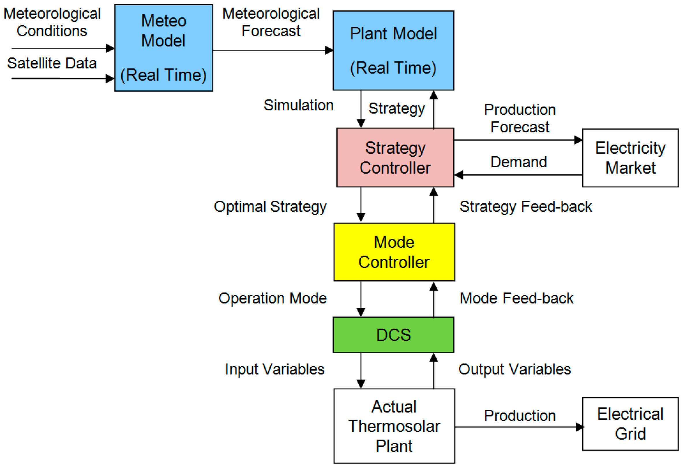
  • Automatic control of the operation mode.
  • Automatic control of the operation strategy.
As already stated, this is the ideal situation for the future; currently, the highest levels of the pyramid in Figure 2 are not automated. The strategy control and the mode control are selected by plant operators that manually run the required simulations and select the strategy to implement and the different modes this strategy goes through. Only the low-level control is implemented in the DCS of the power plant. Some newer plants, like the one in Ouarzazate, Morocco, have succeeded in implementing the Meteo Model and the Plant Model included in Figure 1, but the whole schematic is still to be fulfilled.
The goal of this paper is to use the TES model described in [30] in order to optimize the charge/discharge process of heat storage systems (which corresponds to a low-level variable control) and, hence, contribute to improving the overall efficiency of the solar thermal plant. Additionally, the results obtained will be compared to those obtained in a real plant, which is something researchers rarely have the opportunity to do. By comparing real and simulated data, it will be possible to determine that the results provided by the model can be used to persuade plant CEOs to make decisions (such as selecting the most adequate control strategy for the thermal energy storage system) based on results provided by simulation models. In this work, several control techniques were considered in order to determine the most appropriate strategy. Simulation results and actual measurements for each of these techniques were compared, thus determining the accuracy of the model used for the charge/discharge of the thermal energy storage system.

2. Materials and Methods

TES systems have different operation modes that must be clearly defined before trying to determine the most adequate control method for the TES process. There is not only one type of TES; it is possible to find sensible heat storage, latent heat storage, chemical storage and cascaded storage [6,32], although only some of them are currently feasible [33,34]. Most commercial TES systems consist of: one cold salt tank, one hot salt tank, an HTF-salt exchanger, pumps (to move the molten salt from one tank into the other), pipes and control valves [35]. This is the type of TES considered in this paper, although one-tank TES are also very popular in the literature [36,37,38]. It must be noticed that the use of TES is not limited to solar thermal plants: they can be integrated in other systems such as oil-fired conventional power plants [39], nuclear power plants [40] or many other applications such as hot water supply, air conditioning, heat pumps, buildings, cogeneration, etc. [41].
Figure 3 shows a schematic representation of the disposition of the TES in a solar thermal plant. This type of representations is widely accepted in literature [2,28,42] to represent the three main circuits in plants of this kind: the solar field (SF), through which the heat transfer fluid (HTF) circulates, the power block, which circulates water and steam, and the TES system.
The performance of a TES system defines three possible operation modes: charge, discharge and idle mode. For the sake of simplicity, the present work will only consider the discharge process to illustrate the performance of the different control methods presented; the charge process performs similarly. As far as the idle mode is concerned, no control is required related to the thermal energy storage. It is true that during this mode the temperature of the molten salt must be observed in order to guarantee that it is always above its freezing temperature. Should the salt temperature drop below the minimum permissible value, security measures will be taken: if temperature reaches 260 °C, a set of heating resistors attached to the tank will be turned on until the temperature is measured to be 265 °C; rather than a control strategy, this is simply an on-off security system with hysteresis.
All the simulation and modelling work presented in this paper has been developed using MATLAB-Simulink R2012b. This software package has also been used in other works [43,44,45], but the equations and methodology described could be easily adapted to any other simulation environment. Figure 4 shows a Simulink block representation of the discharging process. A description of the signals associated to this block can be found in Table 1, Table 2 and Table 3: input variables, perturbation variables affecting the process and output variables. All these variables are associated to the area labeled TES in Figure 3; output variables and perturbations are involved in the operation of the heat exchanger, whereas input variables determine the operation of the valves that allow circulation from one salt tank to the other [30].
All these variables were adequately included in the model that will be used throughout this paper to test different control strategies. The discharge process is meant to transfer the heat stored in the hot salt to the HTF in order to make it hot enough to be used in the water-steam cycle. Therefore, the goal during this operation mode is regulating temperature THTFH. This must be achieved by conveniently determining the set points for the valves in the system, SPOC and SPOR, and the set points for the frequency converters of the pumps, SPVHi; perturbations must also be taken into account, and other output variables must also be observed to gain insight into what is actually happening. This model has already been validated in [30] by considering simple control methods: a semiautomatic control and a PID regulator. In the present paper more advanced control solutions will be tested.

2.1. Control Strategies Considered

Three different alternatives will be considered to control the TES system:
  • PID control with feed-forward
  • Advanced PID control with feed-forward
  • Adaptive-predictive control with feed-forward
Other control strategies might have been analyzed as well. Particularly, the non-adaptive predictive control has been disregarded because this control strategy does not perform well when the process is either non-linear or changing, which happens to be the case of the system to be dealt with in this paper.

2.1.1. PID Control with Feed-Forward

The PID control with feed-forward improves the performance of a simple PID regulator by correcting the influence of the perturbations of the process. This is done by using the perturbations themselves to estimate the set point for the control variables of the process. In this paper, such estimation is done by using equations associated to the steady-state operation of the process. It must be noted that feed-forward control is only possible if two conditions are met:
  • Perturbations are measurable.
  • The equations relating the perturbations and the control variables of the process to be regulated are known.
For the case of the discharge process, the first condition is met, since all the three perturbations affecting the process, TSaltH, THTFC and the mass flow of cold HTF in the heat exchanger, m ˙ H T F C can be measured.
The second condition also applies, since application of the first law or thermodynamics to the heat exchangers results in a steady-state equation that allows the mass flow of salt to be estimated as a function of enthalpy as indicated in (1). This estimated value contributes to a better definition of the set point for the salt mass flow, SP, which controls the discharge process:
m ˙ S a l t _ C A L = m ˙ H T F C × ( h H T F H h H T F C ) P h * S a l t H h S a l t C
where hHTFH is the enthalpy of the hot HTF, hHTFC is the enthalpy of the cold HTF, hSaltH is the enthalpy of the hot salt, hSaltC is the enthalpy of the cold salt and P represents the thermal losses in the trains of the heat exchanger. Note that enthalpies are a function of temperature, as indicated in (2); since the temperature of the hot salt is the output of the process, the value hSaltH in this expression is calculated by using the set point for the hot salt temperature.
h H T F H = h H T F ( T H T F H ) h H T F C = h H T F ( T H T F C ) h S a l t C = h S a l t ( T S a l t C ) h * S a l t H = h S a l t ( S P T S a l t H )
Figure 5 shows the Simulink block diagram associated to a PID control with feed-forward. Equation (1) is included in the block labeled “Enthalpic Balance”, which is the only addition to a traditional PID regulator.

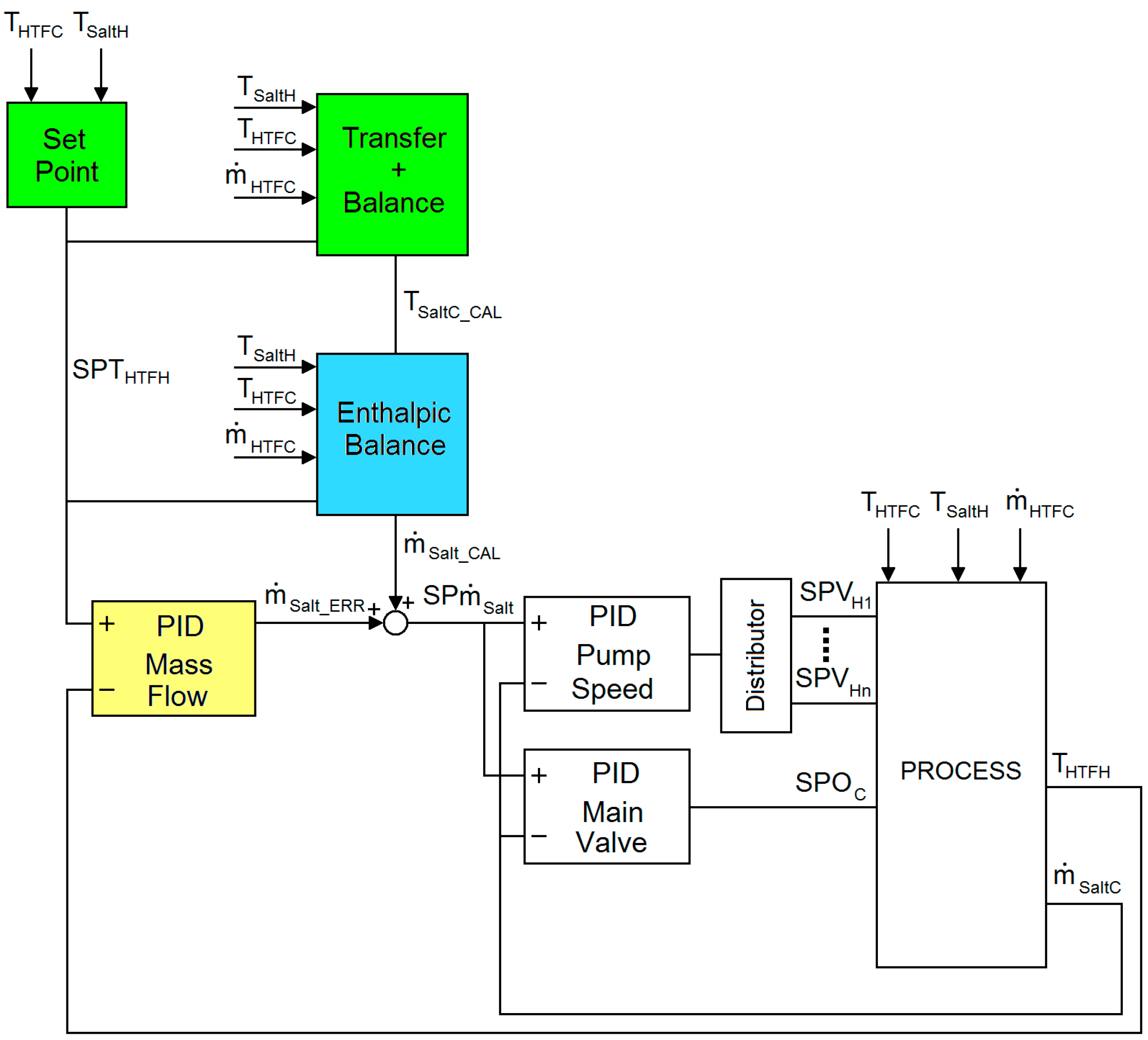
2.1.2. Advanced PID Control with Feed-Forward

This control strategy follows the same idea as the one described in Section 2.1.1, with two improvements introduced:
  • Estimating the temperature reference, i.e., the set point for the hot-HTF temperature, SPTHTFH.
  • Estimating the temperature of the cold salt, TSaltC_CAL, at the output of the heat exchanger.
For the case of the discharge process, estimation of the set point for the hot-HTF temperature (SPTHTFH) starts by considering the nominal values of the temperatures at the input and the output of the heat exchanger during the discharge process: THTFH,nom, THTFC,nom, TSaltH,nom and TSaltC,nom. Using these values, the nominal temperature approach during the discharge process is calculated:
T A , n o m = T S a l t H , n o m T H T F H , n o m
Next, the approach factor during discharge is calculated as the ratio difference between hot salt temperature and cold HTF temperature to its nominal value:
F A , n o m = T S a l t H T H T F C T S a l t H , n o m T H T F C , n o m
This factor is used to calculate the approach of hot temperatures, TA:
T A = F A , n o m × T A , n o m
From here, the reference temperature of the hot salt can be obtained as follows:
S P T H T F H = T S a l t H T A
The second improvement consists of using a better estimation of the cold salt temperature that will be used to calculate the mass flow. The PID converter with feed-forward uses the actual cold salt temperature, TSaltC, measured at the output of the system, but this value does not necessarily correspond to the final value to be obtained in steady state. A steady-state estimation, TSaltC_CAL, can be obtained for that purpose by considering the heat transfer equation inside the heat exchanger:
Q ˙ = Q ˙ ( S P T H T F H , T H T F C , T S a l t H , T S a l t C _ C A L ) = U × S × ( S P T H T F H T S a l t C _ C A L ) ( T S a l t H T H T F C ) ln ( S P T H T F H T S a l t C _ C A L T S a l t H T H T F C )
where U is the global heat transmission coefficient measured for the heat exchanger and S is the exchange area; and the enthalpy balance resulting from the principle of conservation of energy
Q ˙ = m ˙ H T F C × ( h * H T F H h H T F C )
where, again, the enthalpies are a function of temperature and hHTFH must be calculated using the set point for the hot HTF temperature.
h H T F C = h H T F ( T H T F C ) h * H T F H = h H T F ( S P T H T F H )
By iteration of these equations, both Q ˙ and TSaltC_CAL can be obtained.
The Simulink block diagram associated to this type of control can be seen in Figure 6. The two improvements described above are included in the boxes labeled “Set Point” and “Transfer + Balance”.

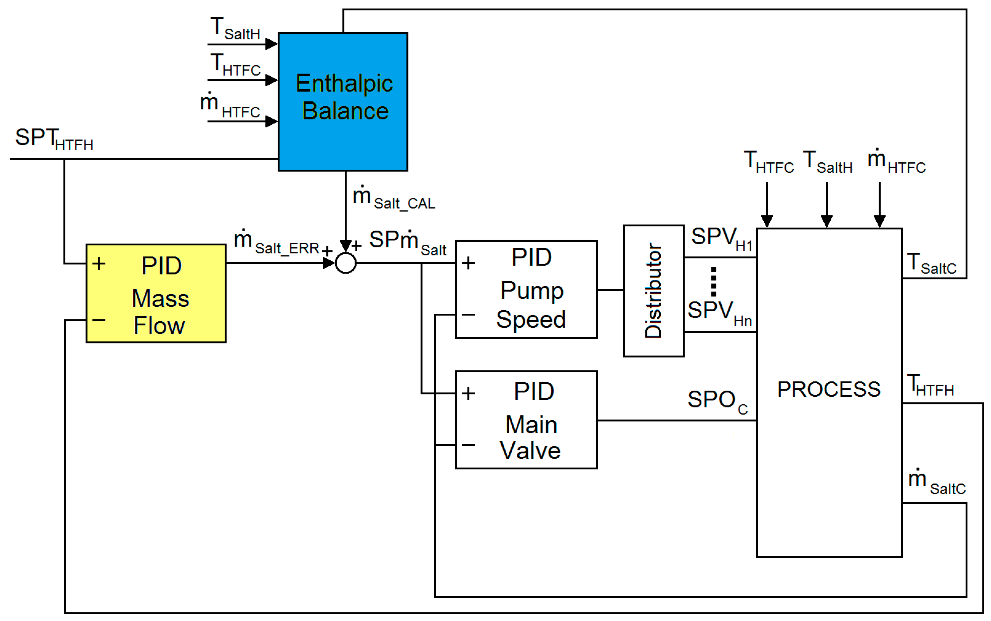
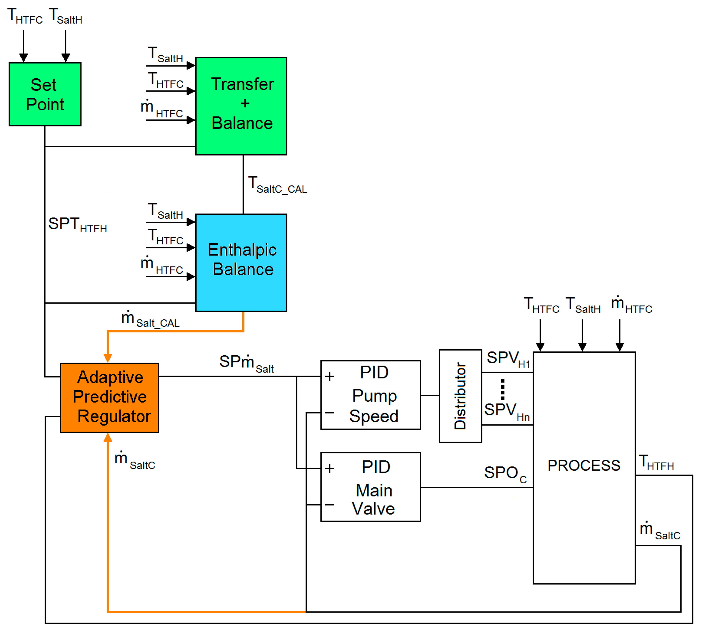
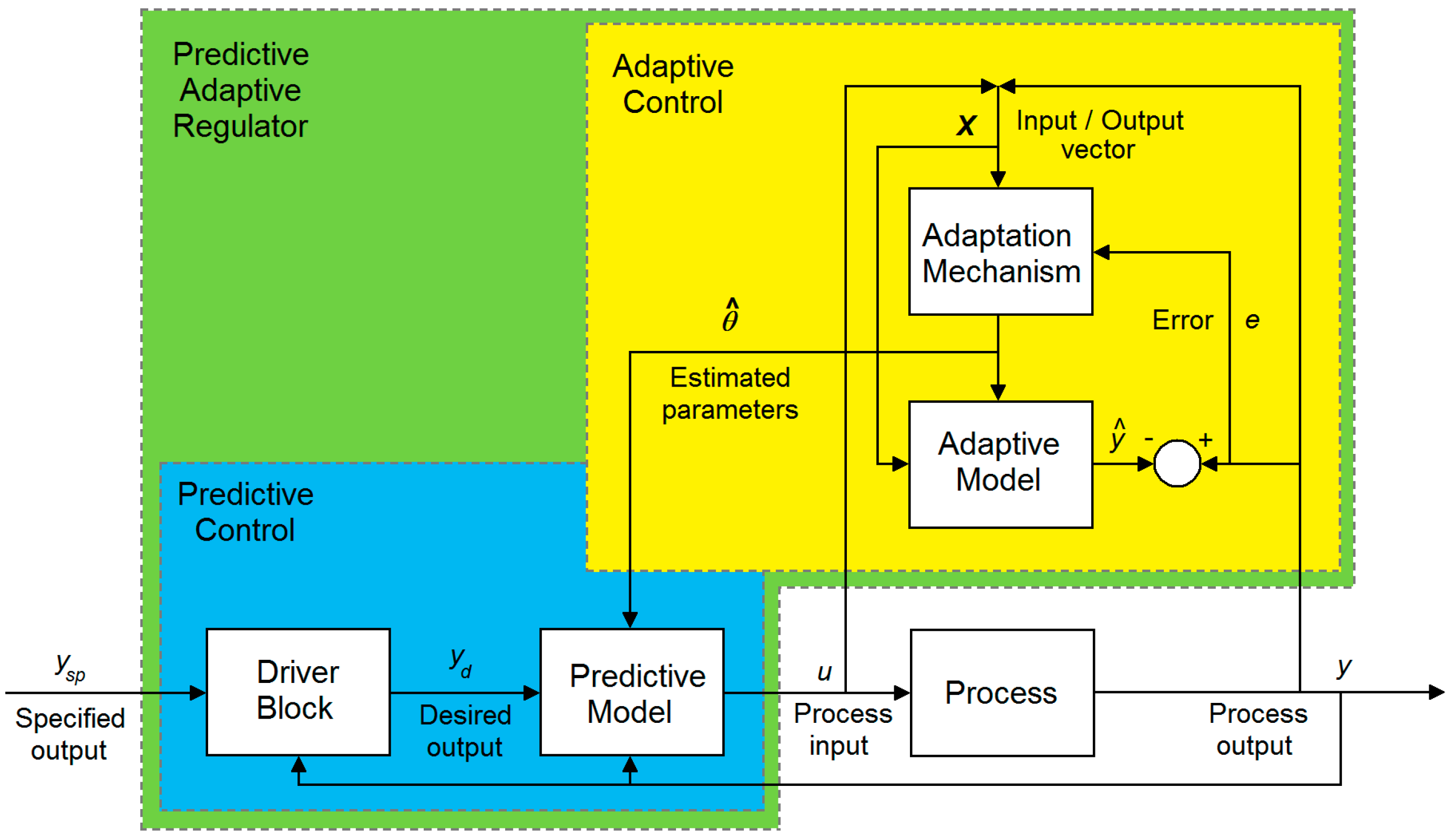
2.1.3. Adaptive-Predictive Control with Feed-Forward

In this control method, represented in Figure 7, the PID block for the mass flow is replaced by a regulator implementing an adaptive-predictive control.
The adaptive-predictive control used is based on that described in [46,47,48], which has already been used in other applications such as wastewater treatment plants [49,50], clinker coolers [51] or electrical grids [52]. However, some modifications have been introduced, namely:
  • The estimated salt flow, m ˙ S a l t _ C A L , is now a perturbation signal for the regulator, which allows for the dynamics of such a perturbation to be considered by the control system.
  • The actual value of the control variable, m ˙ S a l t C , is measured and fed back into the regulator. This allows the system to include the dynamics of the other PID regulators (valves, frequency converters of the pumps).
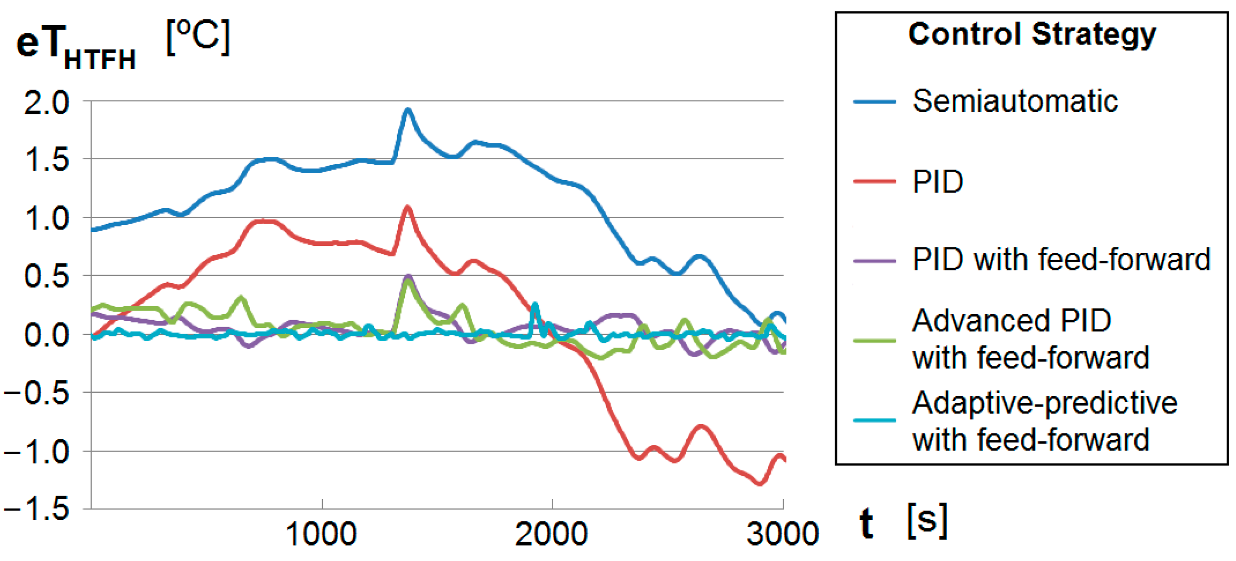
A predictive control must generate the input to the process taking into account the value expected at the output. This means that the transfer function of this regulator must be the inverse of that of the process. Therefore, this control requires that the process model be expressed as a transfer function defined in terms of a set of estimated parameters. The problem of this type of control is that it cannot be used if the parameters of the process change with time, which is the case of the system considered in this work.
Adaptive control consists in adjusting the regulator parameters as a function of the performance of the process. The evolution of inputs and outputs is analyzed in order to optimize the regulator. This allows the control system to be optimally used with processes that change their operation with time. However, this type of control does not allow an expected evolution of the outputs to be defined.
Aiming to overcome the weaknesses of the two strategies described above, adaptive-predictive control combines the features of both systems while avoiding their limitations. The one used in this paper can be considered as a predictive control in which the parameters of the process are estimated by means of an adaptive control of the type STR (self-tuning regulator) [53]. The block diagram of such a regulator is shown in Figure 8.
Formulation of this type of control is somewhat lengthy. It must be noted, though, that the goal of this paper is not actually developing an optimized specific control strategy for the TES system, but determining the results that can be expected when using different control methods existing in literature and comparing them to real results obtained from a power plant. The adaptive-predictive regulator tested in this work follows the concept explained in [54].
The driver block in Figure 8 tries to make the desired output, yd, match the reference specified, ysp, while following a known trajectory (typically linear). The transfer function that relates both magnitudes is chosen to be a second-order, critically damped one with unity gain, which results in a difference equation of the type indicated in (10), where yd has been replaced by the actual output value, y, for samples previous to the current one:
y d ( k ) = α 1 × y ( k 1 ) + α 2 × y ( k 2 ) + β 1 × y s p ( k 1 ) + β 2 × y s p ( k 2 )
The Predictive-Model block must produce the input to the process, u, considering the desired output, yd, the actual output value, y, and a set of estimated parameters, θ ^ , provided by the adaptive block. Equation (11) is a possible implementation of this block:
u ( k ) = u ^ ( k | k ) = y d ( k + λ | k ) i = 1 n ^ e ^ i ( λ ) ( k ) × y ( k + 1 i ) i = 2 m ^ g ^ i ( λ ) ( k ) × u ( k + 1 i ) i = 1 λ g ^ 1 ( i ) ( k )
where k is the current sample considered and λ is the number of future samples to calculate; functions e ^ i and g ^ i are provided by the adaptive control and depend on the prediction error found at instant k.

3. Results

3.1. Simulation of the TES-System Control Strategies

All the control strategies presented in this paper were tested with the model described in [30]. The simulation tests carried out start by adjusting the parameters of the process, which is done by using measurements in an actual plant so that the model is as precise as possible. Two types of measurements are made: measurements for estimation of parameters and measurements to simulate perturbations. First, temperatures, mass flow and other magnitudes that determine the parameters associated to the TES system are measured; these values contribute to the final definition of the model: transmission coefficient, thermal inertia. After these measurements have been made, the regulator parameters are adjusted so that the results obtained also match accurately the ones measured. Finally, the values measured for the perturbations are applied in the simulation and the results obtained are analyzed; all the magnitudes designed as perturbation in the model are measured in representative periods of the discharge so that they can be included in the simulation and check the accuracy of the model response).
As already indicated, the output to be considered during the discharge of a TES system is the temperature of hot HTF, THTFH. Evaluation of the performance of the different control strategies is made by considering the difference between the temperature value obtained at the output and the set point for this magnitude, eTHTFH:
e T H T F H = T H T F H S P T H T F H
A simulation was run for each of the five control strategies indicated in the figure. The set point for the temperature of hot HTF was SPTHTFH = 380°C. Each simulation produced a prediction of the evolution of the actual temperature, THTFH, as a function of time. The curves in Figure 9 show a representative 3000-second sample of the evolution of the error obtained for each control strategy. The closer these curves are to zero, the better the performance of the control strategy considered.
This error was quantified by means of the average deviation, µ, and the standard deviation, σ, which were calculated as follows:
μ = t S T A R T t E N D e T H T F H d t t E N D t S T A R T
σ = t S T A R T t E N D ( e T H T F H μ ) 2 d t t E N D t S T A R T
Table 4 represents the average and standard deviation associated to the error in THTFH. The results in this table are graphically represented in Figure 10.
According to these results, the most suitable control strategy would be an adaptive-predictive control with feed-forward, for it would allow the set point to be followed more accurately. This is the point where most research works finish because power plant CEOs are seldom willing to try modifications in running plants. In this work, however, the authors had the opportunity to validate the model and several control strategies under real working conditions, so that it was possible to determine whether they match the system under consideration.

3.2. Experimental Results

In this section the simulation results just obtained are compared with actual plant measurements carried out in two 50-MW PTC thermal plants built by Group TSK in 2010–2011, with a TES capacity of 7 h: “SAMCA2-La Dehesa” and “La Africana”. The comparison was established by considering the net energy generated by the thermal plant during the discharge of the TES.
Permission to obtain experimental results in the plants was only granted if actual measurements were carried out guaranteeing that there would be no interference with energy production. Taking this into account, the tests were performed according to the following procedure:
  • Tests are to be performed on summer sunny days, when there is an excess of solar energy that cannot be used in the turbine and, therefore, must be stored.
  • Each test lasts for a whole day during which the TES system is fully charged and then fully discharged.
  • Since daily conditions may differ from one test to another, all the control strategies are tested several times so as to reduce the influence of such variable conditions.
  • When the discharge begins, the plant counter of energy sold is consulted.
  • The TES is fully discharged while the turbine is operating at full power. If at the end of the discharge the salt level in the hot tank is higher than one meter, the discharge will be considered to be incomplete and the test will be disregarded.
  • At the end of the discharge, the plant counter of energy sold is read again. The difference between this reading and the one made at the beginning of the discharge will provide the net energy generated with the control strategy under test. The net energy provided during these discharges will be used to evaluate the performance of the control strategy implemented.
  • For every successful discharge, the most relevant meteorological conditions during the test are written down for later use in simulations.
It must be noted that the model described in Section 2 to determine the most suitable control strategy for the thermal energy storage system is only focused on this part of the process and does not, therefore, provide information of the net energy generated in the power plant. Thus, experimental results will be compared to those offered by a commercial plant model that includes the control strategies to evaluate.
The software used in “SAMCA2-La Dehesa” is called ESEMpro® 1.0 and has been developed by S2M (Sun To Market Solutions, Madrid, Spain). This software is fed with the same conditions as those in the real plant test and with different control strategies for the TES system. Table 5 shows how both results (actual and simulated) compare when used to determine the total net energy produced after seventeen complete discharges.
The values included in Table 5 show that the best result is obtained when an adaptive-predictive control with feed-forward is implemented, as anticipated by the simulation results provided by the TES model considered. The amount of net energy generated from 17 full discharges of the TES system using this control strategy gives rise to an increase of 3.6% as compared to that obtained with a PID control (the one actually implemented in the power plant used for the tests).
Additionally, the last column in this table proves that the ESEMpro® model used for the plant can be trusted, for it exhibits good accuracy: the simulated results match those measured in the actual plant with a precision better than 0.3%. It can be noticed that, the more complex the control considered, the larger the error, but even in that case the error produced is within narrow tolerance.

4. Discussion

Using a model of a thermal energy storage (TES) system for power plants, several control methods were tested. Five different strategies were compared: the so-called semiautomatic control system, a simple PID control, a PID control with feed-forward, an advanced PID control with feed-forward and an adaptive-predictive control with feed-forward. All of these control techniques were evaluated with the Simulink TES model developed in [30], which evinced that the best results were obtained when an adaptive-predictive control with feed-forward was implemented.
The opportunity to test the control strategies on a real plant allowed researchers to further verify that implementing such a control in the thermal energy storage system actually resulted in an increase of the energy produced when using the heat stored in the molten salts. Thus, the main goal of this paper could be fulfilled: encouraging plant managers to try different control strategies based on reliable simulation results, like those used in this paper (TES model presented in [30] or ESEMpro®).

5. Conclusions

The discussion above aims to clarify that the final contribution of this paper is not introducing an optimum control strategy for the thermal energy storage system in solar plants, but validating the results provided by certain simulation models in order to encourage the CEOs of solar thermal power plants to rely on the information provided by these models to make their decisions.
To achieve this goal, the present work used the model of a TES system already available in the literature [30] to run several simulations with different control strategies (PID with feed-forward, advanced PID with feed-forward and adaptive-predictive control with feed-forward). The results obtained from these simulations determined which of the control methods considered gave rise to the minimum error and should, therefore, be implemented.
The results obtained were validated by performing actual tests in two 50-MW PTC thermal plants built by Group TSK in 2010–2011, with a TES capacity of 7 h: “SAMCA2-La Dehesa” and “La Africana”. The comparison was established on the grounds of net energy produced during the discharge process, and the experimental results agreed well with the simulations run previously: the control strategy that gave rise to the lowest error was also the control strategy providing the highest net energy during the discharge.
These results contribute to the automation of the plant, since the control strategies identified as optimal can be implemented in the DCS of the solar thermal power plant, thus avoiding the need for operators that might make a wrong decision or react too late to certain changes.
As for the future work, the possibility to increase the automation of the whole plant should be explored, trying to develop algorithms that allow the most adequate global strategy to be selected in terms of meteorological conditions and also considering the conditions set by the electrical market at a given time. This global strategy would consist of several operation modes that should be run in a sequence to be determined by another algorithm still to be developed as well.
It must be said, however, that there must be an afterword to all this. It is true that, as proven in this work, plant CEOs would do well to rely on simulation results to improve production. It is also true that, technically speaking, some control strategies may prove more efficient than others; in this case, it has been demonstrated that using an adaptive-predictive control with feed-forward in the TES system gives rise to an increase in the energy produced during a discharge. But there are other non-technical considerations that managers must also take into account.
In this case, for instance, developing an adaptive-predictive regulator ad-hoc in the distributed control system (DCS) of the plant is not advisable because of its complexity: an external commercial regulator should be used instead. Using a commercial adaptive-predictive regulator in the DCS has some advantages (reduction of development and implementation times, externalized code maintenance, very optimized code, product actualization) but it has some drawbacks too (dependence on a hardware external to the DCS, dependence on an external software with unknown code).
Also, economic implications must be considered. According to the results provided by the models used, the net benefit obtained over 25 years if an adaptive-predictive control with feed-forward were implemented in the TES system, would be around $1,000,000 (as compared to having a PID regulator). Large as it may seem, this benefit is only 0.1% of the total benefit obtained in the power plant, which might not justify the increase of the complexity of the algorithm or the reduced controllability of the whole system (associated to the use of external hardware and software). This risk factor could well result in selecting the advanced PID regulator with feed-forward as the best solution out of those analyzed. In addition, this type of controller is cheaper than one implementing adaptive-predictive control with feed-forward. Considering licenses, initial tests and training of the operators in charge of controlling the plant, the investment associated to including adaptive-predictive control with feed-forward in the TES system has been estimated to be around $13,500, whereas that corresponding to an advanced PID regulator with feed-forward would only be approximately $3500.
This is true for any given high-level strategy used in the plant, i.e., the figures indicated above represent the benefit associated to using one discharge control or another once the global strategy controller has decided the actions to take in the power plant. This is why the contribution of the so-called variable control (see Figure 2) to the overall benefit of the plant is so reduced.

Acknowledgments

Financial support was provided by the Spanish Government through Project MINECO-17-TEC2016-77738-R and by Principado de Asturias (Spain) through Project FC-15-GRUPIN14-122.

Author Contributions

This paper is part of the PhD Thesis developed by Rogelio Peón Menéndez [55], who has therefore carried out most of the work presented here. Juan Á. Martínez and Miguel J. Prieto were the supervisors of this work, whereas Lourdes Á. Barcia and Fernando Nuño respectively assisted Rogelio Peón with Simulink simulations and regulation topics.

Conflicts of Interest

The authors declare no conflict of interest.

References

  1. British Petroleum. BP Statistical Review of World Energy 2016; BP p.l.c.: London, UK, 2016. [Google Scholar]
  2. Yang, Z.; Garimella, S.V. Cyclic operation of molten-salt thermal energy storage in thermoclines for solar power plants. Appl. Energy 2013, 103, 256–265. [Google Scholar] [CrossRef]
  3. Usaola, J. Operation of concentrating solar power plants with storage in spot electricity markets. IET Renew. Power Gener. 2012, 6, 59–66. [Google Scholar] [CrossRef]
  4. Lillo, I.; Pérez, E.; Moreno, S.; Silva, M. Process Heat Generation Potential from Solar Concentration Technologies in Latin America: The Case of Argentina. Energies 2017, 10, 383. [Google Scholar] [CrossRef]
  5. Hassine, I.B.; Sehgelmeble, M.C.; Söll, R.; Pietruschka, D. Control optimization through simulations of large scale solar plants for industrial heat applications. Energy Procedia 2015, 70, 595–604. [Google Scholar] [CrossRef]
  6. Tian, Y.; Zhao, C.Y. A review of solar collectors and thermal energy storage in solar thermal applications. Appl. Energy 2013, 104, 538–553. [Google Scholar] [CrossRef]
  7. Zhang, H.L.; Baeyens, J.; Degrève, J.; Cacères, J. Concentrated solar power plants: Review and design methodology. Renew. Sustain. Energy Rev. 2013, 22, 466–481. [Google Scholar] [CrossRef]
  8. Kaltschmitt, M.; Wolfgang, S.; Andreas, W. Solar Thermal Power Plants. In Renewable Energy; Springer: Berlin/Heidelberg, Germany, 2007; pp. 171–228. [Google Scholar]
  9. Schnatbaum, L. Solar thermal power plants. Eur. Phys. J. Spec. Top. 2009, 176, 127–140. [Google Scholar] [CrossRef]
  10. Wu, S.Y.; Xiao, L.; Cao, Y.; Li, Y.R. A parabolic dish/AMTEC solar thermal power system and its performance evaluation. Appl. Energy 2010, 87, 452–462. [Google Scholar] [CrossRef]
  11. Saleem, S.; Asar, A. Analysis & Design of Parabolic Trough Solar Thermal Power Plant for Typical Sites of Pakistan. IOSR J. Electr. Electron. Eng. (IOSR-JEEE) 2014, 9, 116–122. [Google Scholar]
  12. Silva, R.; Cabrera, F.J.; Pérez-García, M. Process heat generation with parabolic trough collectors for a vegetables preservation industry in Southern Spain. Energy Procedia 2014, 48, 1210–1216. [Google Scholar] [CrossRef]
  13. Jebasingh, V.K.; Joselin Herbert, G.M. A review of solar parabolic trough collector. Renew. Sustain. Energy Rev. 2016, 54, 1085–1091. [Google Scholar] [CrossRef]
  14. Lamba, D.K. Review on Parabolic Trough Type Solar Collectors: Innovation, Applications and Thermal Energy Storage. In Proceedings of the National Conference on Trends and Advances in Mechanical Engineering, YMCA University of Science & Technology, Faridabad, Haryana, 19–20 October 2012. [Google Scholar]
  15. Desai, N.B.; Bandyopadhyay, S. Optimization of concentrating solar thermal power plant based on parabolic trough collector. J. Clean. Prod. 2015, 89, 262–271. [Google Scholar] [CrossRef]
  16. Eck, M.; Hennecke, K. Heat Transfer Fluids for Future Parabolic Trough Solar Thermal Power Plants. In Proceedings of the ISES World Congress, Beijing, China, 18–21 September 2007. [Google Scholar]
  17. Ter-Gazarian, A.G. Thermal Energy Storage. In Energy Storage for Power Systems, 2nd ed.; IET Press: Stevenage, UK, 2011; pp. 55–76. [Google Scholar]
  18. Chen, H.; Cong, T.N.; Yang, W.; Tan, C.; Li, Y.; Ding, Y. Progress in electrical energy storage system: A critical review. Prog. Nat. Sci. 2009, 19, 291–312. [Google Scholar] [CrossRef]
  19. Luo, X.; Wang, J.; Dooner, M.; Clarke, J. Overview of current development in electrical energy storage technologies and the application potential in power system operation. Appl. Energy 2015, 137, 511–536. [Google Scholar] [CrossRef]
  20. 20 MW/80 MWh-Energy Nuevo-Amber Kinetics, “DOE International Energy Storage Database”. Available online: http://www.energystorageexchange.org/projects/1975 (accessed on 6 July 2017).
  21. Central Hidroeólica de El Hierro, “Noticias del Meridiano”. Available online: http://www.elhierro.tv/noticias/008_01_20/008_01_20.html (accessed on 6 July 2017).
  22. Markersbach Pumped Storage Power Plant, “DOE International Energy Storage Database”. Available online: http://www.energystorageexchange.org/projects/402 (accessed on 6 July 2017).
  23. 110-Megawatt Compressed Air Energy Storage facility, “Power South Energy Cooperative”. Available online: http://www.powersouth.com/mcintosh_power_plant/compressed_air_energy (accessed on 6 July 2017).
  24. Southern California Edison-Chino Battery Storage Project, “DOE International Energy Storage Database”. Available online: http://www.energystorageexchange.org/projects/2186 (accessed on 6 July 2017).
  25. Laing, D.; Steinmann, W.D.; Tamme, R. Sensible Heat Storage for Medium and High Temperatures. In Proceedings of the ISES World Congress, Beijing, China, 18–21 September 2007. [Google Scholar]
  26. Goods, S.H.; Bradshaw, R.W. Corrosion of stainless steels and carbon steel by molten mixtures of commercial nitrate salts. J. Mater. Eng. Perform. 2004, 13, 78–87. [Google Scholar] [CrossRef]
  27. USA Trough Initiative. Thermal Storage Oil-to-Salt Heat Exchanger Design and Safety Analysis; Task Order Au. No. KAF-9-29765-09; Nexant Inc.: San Francisco, CA, USA, 2000. [Google Scholar]
  28. Llorente García, I.; Álvarez, J.L.; Blanco, D. Performance model for parabolic trough solar thermal power plants with thermal storage: Comparison to operating plant data. Sol. Energy 2011, 85, 2443–2460. [Google Scholar] [CrossRef]
  29. Powell, K.M.; Edgar, T.F. Modeling and control of a solar thermal power plant with thermal energy storage. Chem. Eng. Sci. 2012, 71, 138–145. [Google Scholar] [CrossRef]
  30. Menéndez, R.P.; Martínez, J.Á.; Prieto, M.J.; Barcia, L.Á.; Sánchez, J.M.M. A Novel Modeling of Molten-Salt Heat Storage Systems in Thermal Solar Power Plants. Energies 2014, 7, 6721–6740. [Google Scholar] [CrossRef]
  31. Peón, R.; Requena, R.; Martín Sánchez, J.M. Optimized Adaptive Control for CSP plants. In Proceedings of the 2nd International Concentrated Solar Power Summit, Madrid, Spain, 5–6 June 2012. [Google Scholar]
  32. Ma, Z.; Glatzmaier, G.; Turchi, C.; Wagner, M. Thermal energy storage performance metrics and use in thermal energy storage design. In Proceedings of the Colorado ASES World Renewable Energy Forum, Denver, CO, USA, 13–17 May 2012. [Google Scholar]
  33. Aneke, W.; Wang, M. Energy storage technologies and real life applications—A state of the art review. Appl. Energy 2016, 179, 350–377. [Google Scholar] [CrossRef]
  34. Mathur, A.; (Terrafore Technologies, Minneapolis, USA). Dynamic Models of Concentrated Solar Power Plant to Response to Utility Demand Profiles. 2014. Available online: http://www.terraforetechnologies.com/wp-content/uploads/2014/02/Dynamic-Models-of-Concentrated-Solar-Power-Plant-to-Response-to-Utility-Demand-Profiles1.pdf (accessed on 6 July 2017).
  35. Torras, S.; Pérez-Segarra, C.; Rodríguez, I.; Rigola, J.; Oliva, A. Parametric study of two-tank TES systems for CSP plants. In Proceedings of the SOLARPACES 2014, Beijing, China, 16–19 September 2014. [Google Scholar]
  36. Modi, A.; Perez-Segarra, C.D. Thermocline thermal storage systems for concentrated solar power plants: One dimensional numerical model and comparative analysis. Sol. Energy 2014, 100, 84–93. [Google Scholar] [CrossRef]
  37. Bayón, R.; Rojas, E. Simulation of thermocline storage for solar thermal power plants: From dimensionless results to prototypes and real-size tanks. Int. J. Heat Mass Transf. 2013, 60, 713–721. [Google Scholar] [CrossRef]
  38. Flueckiger, S.M.; Iverson, B.D.; Garimella, S.V.; Pacheco, J.E. System-level simulation of a solar power tower plant with thermocline thermal energy storage. Appl. Energy 2014, 113, 86–96. [Google Scholar] [CrossRef]
  39. Wojcik, J.D.; Wang, J. Technical Feasibility Study of Thermal Energy Storage Integration into the Conventional Power Plant Cycle. Energies 2017, 10, 205. [Google Scholar] [CrossRef]
  40. Edwards, J.; Bindra, H.; Sabharwall, P. Exergy analysis of thermal energy storage options with nuclear power plants. Ann. Nucl. Energy 2016, 96, 104–111. [Google Scholar] [CrossRef]
  41. Li, G.; Zheng, X. Thermal energy storage system integration forms for a sustainable future. Renew. Sustain. Energy Rev. 2016, 62, 736–757. [Google Scholar] [CrossRef]
  42. Martín, L.; Zarzalejo, L.F.; Polo, J.; Navarro, A.; Marchante, R.; Cony, M. Prediction of global solar irradiance based on time series analysis: Application to solar thermal power plants energy production planning. Sol. Energy 2012, 84, 1772–1781. [Google Scholar] [CrossRef]
  43. Álvarez Barcia, L.; Peón Menéndez, R.; Martínez Esteban, J.Á.; José Prieto, M.Á.; Martín Ramos, J.A.; Cos Juez, F.J.; Nevado Reviriego, A. Dynamic Modeling of the Solar Field in Parabolic Trough Solar Power Plants. Energies 2015, 8, 13361–13377. [Google Scholar] [CrossRef]
  44. Roca, L.; Bonilla, J.; Rodríguez García, M.M.; Palenzuela, P.; Calle, A.; Valenzuela, L. Control strategies in a thermal oil—Molten salt heat exchanger. In Proceedings of the SOLARPACES 2015, Cape Town, South Africa, 13–16 October 2015; American Institute of Physics: Melville, NY, USA, 2016. [Google Scholar]
  45. Qenawy, M. Matlab Simulation of 10 MW Molten Salt Solar Power Tower Plant in Aswan. Noble Int. J. Sci. Res. 2017, 1, 34–43. [Google Scholar]
  46. Martín-Sánchez, J.M.; Rodellar, J. Adaptive Predictive Control: From the Concepts to Plant Optimization, 1st ed.; Prentice Hall: Upper Saddle River, NJ, USA, 1995. [Google Scholar]
  47. Martín-Sánchez, J.M.; Rodellar, J. Control Adaptativo Predictivo Experto: Metodología, Diseño y Aplicación; Universidad Nacional de Educación a Distancia: Madrid, Spain, 2005. [Google Scholar]
  48. Martín-Sánchez, J.M.; Rodellar, J. Estrategia básica de control predictivo. In Control Adaptativo Predictivo Experto ADEX. Metodología, Diseño y Aplicación; UNED: Madrid, Spain, 2005; pp. 83–102. [Google Scholar]
  49. Kandare, G.; Viúdez-Moreiras, D.; Hernández-del-Olmo, F. Adaptive control of the oxidation ditch reactors in a wastewater treatment plant. Int. J. Adapt. Control Signal Process. 2012, 26, 976–989. [Google Scholar] [CrossRef]
  50. Nevado, A.; Requena, R.; Polo, P. Un control adaptativo predictivo experto para una E.D.A.R. Autom. Instrum. 2010, 415, 50–53. [Google Scholar]
  51. Nevado, A.; Requena, R.; Videz, D.; Plano, E. A new control strategy for IKN-type coolers. Control Eng. Pract. 2011, 19, 1066–1074. [Google Scholar] [CrossRef]
  52. Requena, R.; Nevado, A.; Martín, J.M. Control optimizado para la red eléctrica de España. Autom. Instrum. 2009, 407, 14–23. [Google Scholar]
  53. Astrom, K.J.; Wittenmark, B. Adaptive Control, 2nd ed.; Addison-Wesley: Boston, MA, USA, 1995. [Google Scholar]
  54. Adaptive Predictive Control. Available online: http://www.adexcop.com/adaptive (accessed on 6 July 2017).
  55. Peón, R. Optimización del Control del Sistema de Almacenamiento Térmico en Centrales Solares Termoeléctricas. Ph.D. Thesis, Universidad de Oviedo, Asturias, Spain, June 2012. [Google Scholar]
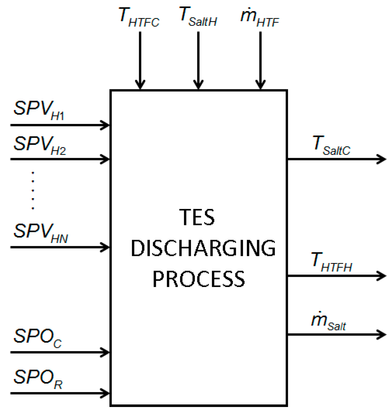
Figure 1. Ideal future block diagram for the control of a solar thermal power plant.
Energies 10 00990 g001
Figure 2. Control pyramid for a solar thermal power plant.
Energies 10 00990 g002
Figure 3. Schematic of a solar thermal power plant.
Energies 10 00990 g003
Figure 4. Process block associated to TES discharging.
Energies 10 00990 g004
Figure 5. PID control with feed-forward (discharge process).
Energies 10 00990 g005
Figure 6. Advanced PID control with feed-forward (discharge process).
Energies 10 00990 g006
Figure 7. Adaptive-predictive control with feed-forward (discharge).
Energies 10 00990 g007
Figure 8. Adaptive-predictive control implemented.
Energies 10 00990 g008
Figure 9. Evolution of the error obtained with different control strategies.
Energies 10 00990 g009
Figure 10. Graphic representation of the simulation results.
Energies 10 00990 g010
Table 1. TES Discharging Input Variables.
Input VariableDescription
SPVHiSet Point for the speed defined by the frequency converter of the i-th hot-salt pump
SPOCSet Point for the opening of the main valve in the cold-salt tank
SPORSet Point for the opening of the recirculation valve
Table 2. TES Discharging Input Perturbations.
PerturbationDescription
THTFCCold HTF temperature at the input of the heat exchanger
TSaltHHot salt temperature at the input of the heat exchanger
m ˙ H T F HTF mass flow through the heat exchanger
Table 3. TES Discharging Output Variables.
Output VariableDescription
THTFHHot HTF temperature at the output of the heat exchanger (variable to control)
TSaltCCold salt temperature at the output of the heat exchanger
m ˙ S a l t Molten salt mass flow through the heat exchanger
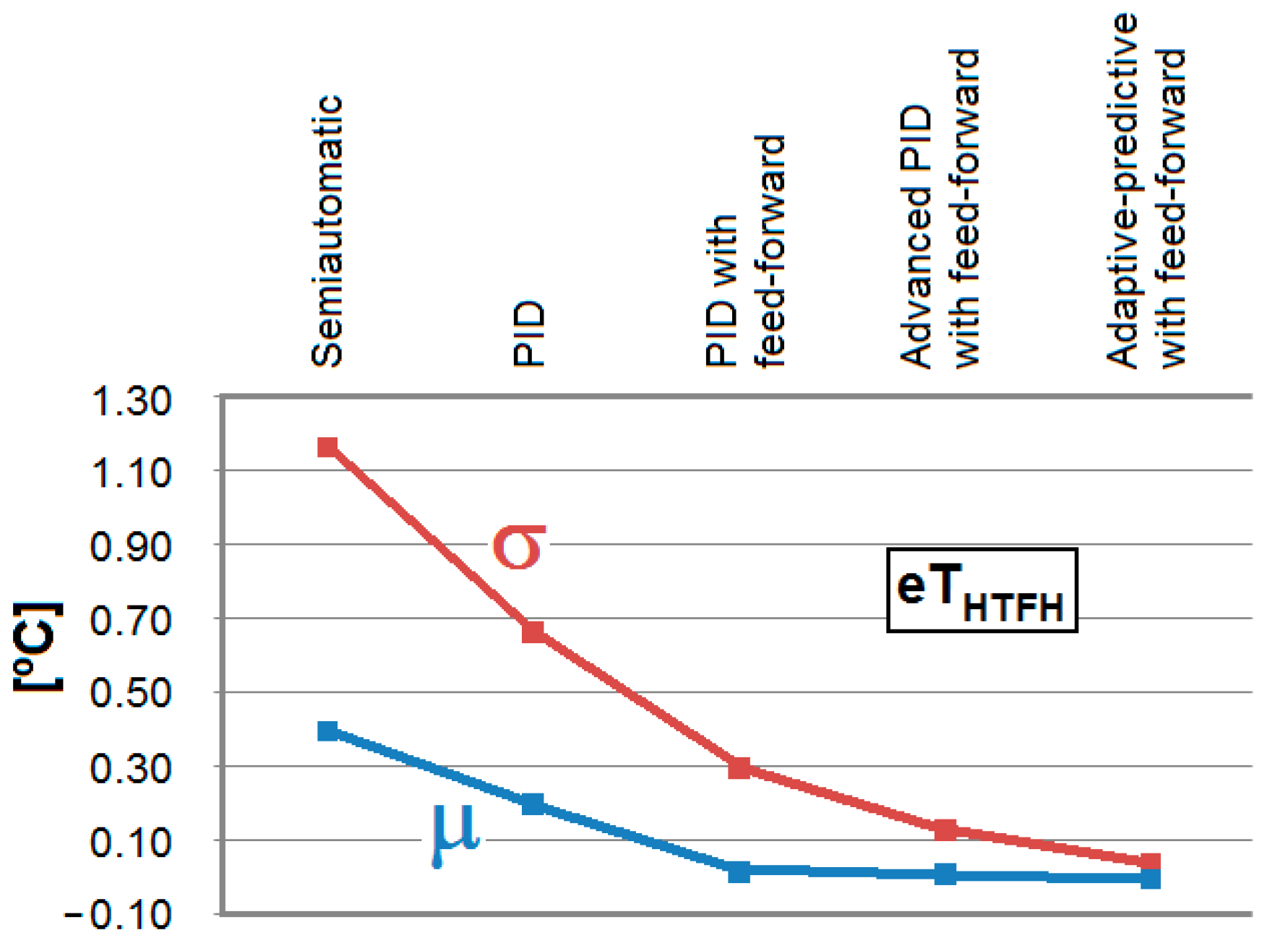
Table 4. TES Discharging Simulation Results.
Control StrategyeTHTFH = THTFHSPTHTFH
μ (°C)σ (°C)
Semiautomatic0.401.17
PID0.200.67
PID with feed-forward0.020.30
Advanced PID with feed-forward0.010.13
Adaptive-predictive with feed-forward0.000.04
Table 5. Net Energy Produced After 17 Discharges.
Control StrategyNet Energy (MW·h)
Real (EN,Real)Simulated (EN,Sim)Difference (%)
Semiautomatic54535458−0.09
PID552255180.07
PID with feed-forward552555140.20
Advanced PID with feed-forward564356280.26
Adaptive-predictive with feed-forward572157050.28

