A Novel Method for Idle-Stop-Start Control of Micro Hybrid Construction Equipment—Part A: Fundamental Concepts and Design

Abstract

Although micro hybrid propulsion (MHP) systems are recognized as a feasible solution for off-highway construction machines (OHCMs), there is still a lack of understanding how existing MHP technologies can be transferred effectively from the automotive sector to the construction sector. To fill this gap, this paper is the first of a two-part study which focuses on micro hybrid construction machines paying attention to a novel idle-stop-start control (ISSC) strategy. Part A presents the system concepts and design procedure while Part B studies on a hardware-in-the-loop test platform for a comprehensive analysis on the potential fuel/emission saving of the proposed system in real-time. In this study—Part A—different types of OHCMs are briefly discussed to identify the target machine. The procedure to model the machine powertrain is also concisely introduced. Next, to minimize the fuel consumption and emissions without degrading the machine performance, a prediction-based idle-stop-start control (PISSC) approach is properly designed. The core of the PISSC is to estimate online the future engine working state changes in order to directly shut down the engine or shift it to low power regions during idle periods. Numerical simulations have been carried out to validate the potential of the proposed PISSC method.

1. Introduction

As reported by the Environmental Protection Agency, the construction industry is identified as the third most significant sector, just behind the oil-and-gas and chemical manufacturing sectors, in terms of having influence on the greenhouse effect. Additionally, the energy crisis is becoming more and more serious while fuel consumption of off-highway construction machines (OHCMs) accounts for a significant portion of total global fuel usage.

In recent years, focusing on hybridisation technologies to reduce fuel consumption and pollutant emissions of both on/off-highway vehicles has become the main policy of governments around the world. Micro hybrid propulsion (MHP), with the main function known as idle-stop-start control (ISSC), is considered one of the most promising solutions for developing low cost powertrains with high energy performance, low fuel use and emissions, while requiring little effort for installation. Acknowledging this secret key as well as realizing the major challenges for the OHCM market, is necessary to explore the feasibility of implementing MHP in this sector.

There have been a number of studies on MHP for applications to the automotive sector [1,2,3,4,5,6,7]. According to different driving conditions, mainly defined by the driver, and forces applied to the brake pedal (for example, stopping/running at traffic lights), the engine can be automatically switched between normal power mode and economic modes, including idle, stop and start, to avoid unnecessary fuel burns [4,5]. In the construction sector, many machines are left running at full power whilst idle for much of their life. In reality during operation of a machine, such as excavator, and particularly at the times of reduced workloads (as load lowering or holding), less than full engine power is required to achieve the desired performance. Such periods of reduced workloads present good opportunities to save fuel and avoid emissions by utilizing a MHP architecture.

Although studies on MHP have been carried out for modern on-road vehicles, there is a very limited amount of research on micro hybridisation in OHCMs. There exists a lack of underpinning knowledge in how the existing MHP technologies can be effectively transferred from the automotive sector to the construction sector to maximize the machine fuel economy and minimize the emissions without sacrificing performance. Compared to on-road vehicles, difficulties in developing OHCMs come from the complex and different architectures leading to different dynamic behaviours and performances. First, it is hard for the operator/controller to detect whether or not a machine has low workloads to reduce the engine power or shut it down to save fuel. Even when staying at a fixed position, the machine may still use the hydraulic actuators on its upper body to perform construction tasks. Second, for any construction task, a machine is normally used with repeatable working cycles where the power requirements are continuously and randomly regulated from high to low levels. Third, the time required to crank a machine’s engine from zero speed to its idle speed is normally longer than that of a vehicle, especially at cold temperatures. Hence, it is necessary to find innovative ISSC solutions for OHCMs to address both these issues.

For the last issue, a proper engine start control approach has been successfully introduced through recent works of the authors [8]. To deal with the first and second issues, several studies on ISSC for OHCMs have been recently proposed to shift the engine working point from the normal power region to the idle power region and vice versa [9,10]. Although these concepts showed the possibility of fuel savings, their applicability has not been investigated. In addition compared to these existing technologies, there is still a high potential to save more energy as well as emissions. For instance, in order to select a suitable mode, normal or economic, the power controller [10] requires a fixed period of time which is long enough to take an observation and perform an analysis on the machine state. This leads to a reduction in the fuel savings whilst idle. In addition, the engine stop-start function has not been taken into account when designing this controller. In another study [9], the engine power can be cut off only in cases the cabin door is opened for either safety or for fuel saving reasons. To the best of the authors’ knowledge, the emerging issues for quickly detecting the engine working states and fully utilizing the ISSC technology in OHCMs have not been addressed.

Therefore, this two-part paper proposes a novel prediction-based idle-stop-start control (PISSC) strategy for the development of greener and more efficient construction equipment. The PISSC is constructed based on a grey prediction model (GPM) and proper logics to select proficiently the engine working modes to minimize the fuel consumption as well as emissions without sacrificing the machine performance. Here, the GPM is capable of estimating online the future engine state changes due to the power demands in order to allow the PISSC to directly shut down the engine or shift it to a low power region during idle periods. For this research objective, Part A mainly outlines the system concepts and procedures to model a machine powertrain and to construct the PISSC scheme while Part B focuses on the real-time evaluation of the proposed methodology in term of fuel and emission reduction.

The remains of this study—Part A—are structured as follows: Section 2 discusses the ability of implementing the ISSC with respect to different types of OHCMs in order to identify the target machine; Section 3 then introduces the procedure to build the powertrain model of the target machine as well as the model parameter setting. The PISSC design is clearly described in Section 4, while numerical simulations have been carried out in Section 5 to investigate the effectiveness of the proposed PISSC method; Concluding remarks are finally given in Section 6.

2. Problem Definition and Selection of Target Machine

Within the global construction market, considerable variations in demand exist among machine types, but by far the most popular types to perform everyday construction work can be recognized as compact excavators, telehandlers, tracked (heavy) excavators, and backhoe loaders [11]. Several analytical studies were carried out with these machine types to evaluate the run time and fuel use during internal combustion engine (ICE) low idle regions. Lewis et al. [12] figured out the idle time ratio was 34% and 32% of the machine life for fleets of heavy excavators and backhoe loaders, respectively. Another study on machine idle was done by JCB—the world’s third largest construction equipment brand by volume, after Caterpillar and Volvo. In this study, a large data set was observed from 2000 random telescopic handlers in the UK using JCB LiveLink software [13] and, the evaluation result of the machine run time and fuel consumption over the full torque-speed range is given in

Table 1. Average engine run time/fuel use against speed-torque range of a telescopic handler.

(% Total Run Time; % Total Fuel Use) of ICE		Engine Speed (rpm)
		0–1000	1000–1250	1250–1500	1500–1750	1750–2000	2000–2250	2250–2500
Torque % of Reference Value	66–100	0.00; 0.00	0.00; 0.00	0.01; 0.03	0.00; 0.04	0.00; 0.00	0.00; 0.00	0.00; 0.00
	60–66	0.00; 0.00	0.00; 0.02	0.10; 0.32	0.23; 0.86	0.01; 0.09	0.00; 0.00	0.00; 0.00
	54–60	0.00; 0.00	0.07; 0.16	0.30; 0.80	0.68; 2.40	0.46; 1.83	0.01; 0.10	0.00; 0.00
	48–54	0.02; 0.04	0.27; 0.52	0.50; 1.19	0.52; 1.55	0.87; 3.28	0.41; 1.67	0.01; 0.04
	42–48	0.21; 0.26	0.43; 0.74	0.54; 1.18	0.57; 1.55	0.32; 1.03	0.52; 2.00	0.24; 0.96
	36–42	0.48; 0.50	0.75; 1.17	0.65; 1.26	0.59; 1.40	0.35; 0.98	0.21; 0.67	0.40; 1.44
	30–36	1.36; 1.32	1.46; 1.97	1.07; 1.80	0.81; 1.63	0.44; 1.05	0.28; 0.75	0.69; 2.17
	24–30	2.72; 2.30	2.24; 2.51	1.72; 2.39	0.91; 1.53	0.53; 1.04	0.32; 0.73	0.98; 2.62
	18–24	8.05; 5.60	3.84; 3.49	1.93; 2.18	1.38; 1.86	0.72; 1.13	0.36; 0.66	0.88; 1.88
	0–18	42.48; 17.34	6.77; 3.59	2.91; 2.22	1.99; 2.01	1.05; 1.38	0.54; 0.98	0.79; 1.77

. As shown in this table, in excess of 42% of the machine life was spent at idle and correspondingly, around 17% of the total fuel consumption was spent during low idle, for very low load tasks or zero productivity.

Based on these analyses, it can be conservatively estimated that a reduction in fuel consumption approaching a minimum of 10% could be realized by shifting the engine working point from the full power region to lower power regions or to shut down it. Such reductions are only achievable if the machine states can be efficiently identified and controlled. This therefore places a high demand on the proposed PISSC technology for the hybridisation of OHCMs.

In order to select a target machine for the PISSC-based MHP development and investigation, it is necessary to take in to account all factors which could have significant impacts on the implementation of MHP. Here, six decisive factors have been selected based on the knowledge from a JCB team expert in machine design and the evaluation of these factors with respect to the most popular machine types is carried out in

Table 2. Evaluation of factors having significant impacts on machine hybridization.

Influential Factor	Compact Excavator	Heavy Excavator	Telescopic Handler	Backhoe Loader
Total idling time over total machine run time	Medium-Low	High	High	Medium
Total fuel in idle over total fuel consumption	Medium-Low	High	High	Medium
Amount of fuel spent in idle	Low	High	High	Medium
Technical ease of installation	Easy	Medium	Difficult	Medium
Payback time	Short	Medium	Medium-Long	Long
Machine potential in market	High	High	High	Medium

.

From this result, it is clear that the highest benefit of employing the PISSC-based MHP can be obtained from heavy excavators. Hence, heavy excavators has been chosen as the target machines and consequently, their architecture is used to develop the PISSC as presented in the following sections.

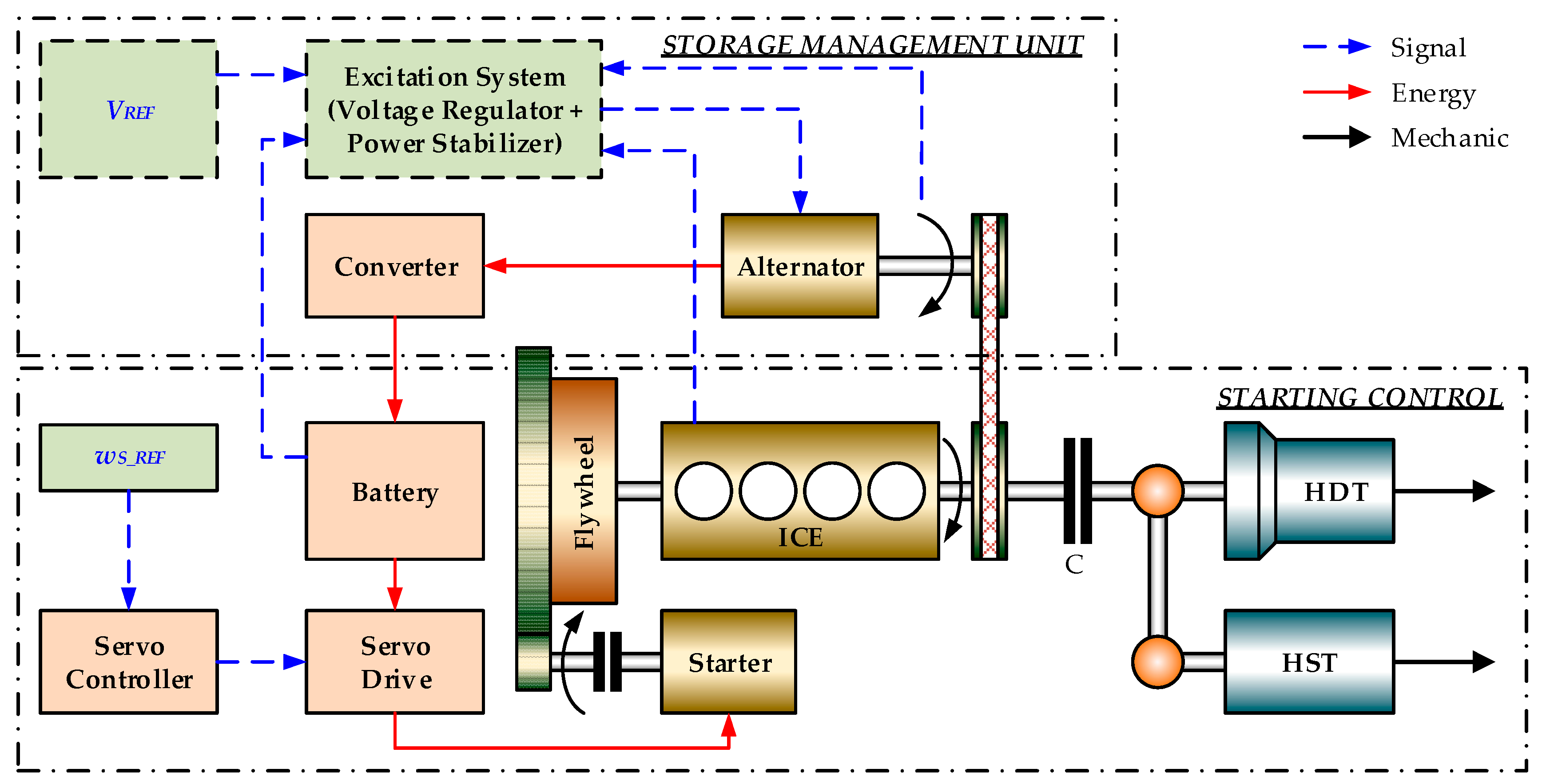
3. Powertrain Model Design

A typical heavy excavator from JCB is targeted for the study and its powertrain is depicted in Figure 1. The powertrain includes an internal combustion engine (ICE), a DC starter, a DC alternator, a lead-acid battery, transmissions and loads. The output shaft of the engine is coupled to the alternator by a belt transmission. The electricity generated by the alternator is stored in the battery which is then used to supply power to the starter to crank the engine. During the ICE cranking phase, the starter-engine engagement is controlled by a pinion-ring gear mechanism and an over-running clutch. A solenoid valve is used to engage the pinion with the ring gear on a flywheel of the engine. The drivetrain, work hydraulics and other auxiliaries can be generally considered as the combination of a hydrodynamic transmission (HDT) and a hydrostatic transmission (HST) which are connected to the engine output shaft through a clutch C (traditionally, a wet clutch).

As stated in the Introduction, this study mainly focuses on the design of the PISSC in which the engine working mode prediction for engine idle-stop-start control algorithms is the core technique. The engine start control method has been successfully built and presented in the recent work published by the authors [8]. Thus, the transient dynamics of the system, including wet clutch dynamics and ICE combustion dynamics, can be neglected for the design of ISSC. In addition, loads coming from the HST and HDT can be represented by a time-variant dynamic load connected to the engine output shaft. Specifications of the main components of this powertrain are given in

Table 3. Specifications of the powertrain’s main components.

Component	Specifications
Belt transmission	Transmission ratio 2.8:1
Pinion-ring gear transmission	Transmission ratio 11:1
	Flywheel mass 44.7 kg
Engine	Four-stroke diesel engine 1.9 L Max speed 2400 rpm Gross power 41 kW, net power 38.4 kW Compression ratio 16.7:1
Starter	12 V working voltage 2 kW power
Alternator	Current 80 A
Battery	Lead-acid battery 12 V nominal voltage 75 Ah capacity

[8].

The powertrain is then modelled as a combination of sub-models, consisting of transmission sub-models, engine sub-model, and electrical components’ sub-models. To reduce the computational effort, the powertrain model is developed by using the mean-value modelling approach and a co-simulation based on MATLAB (MathWorks, Natick, MA, USA) and AMESim (Siemens, Munich, Germany). Herein, the engine, starter, transmissions and mechanical loads are modelled using AMESim while the battery, alternator and electrical load are modelled in MATLAB/Simulink using Simscape.

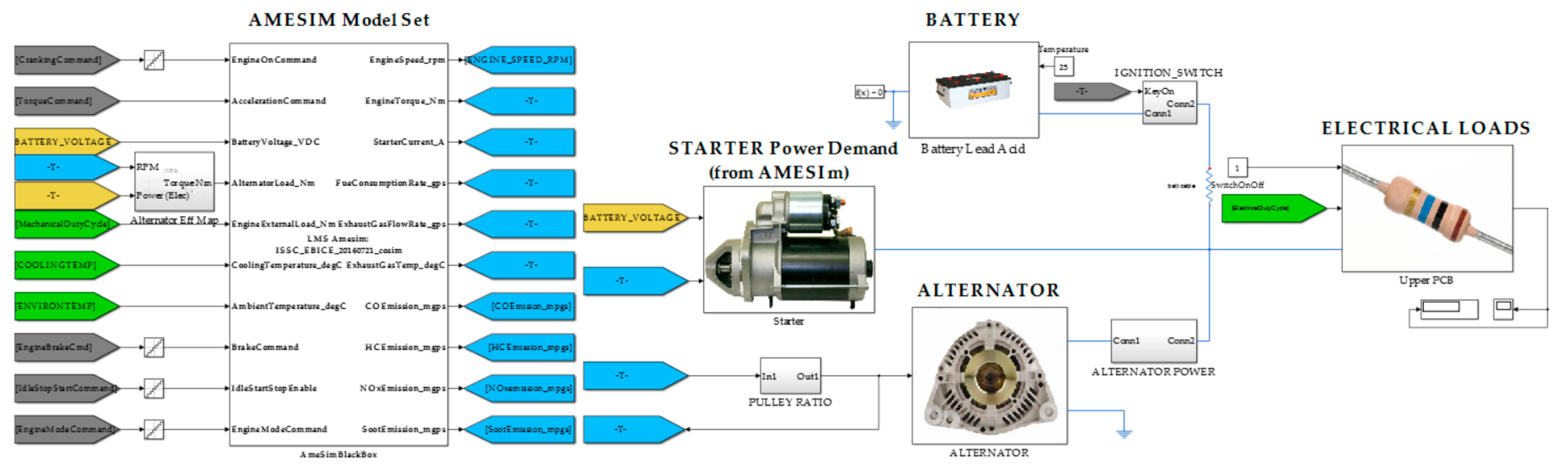
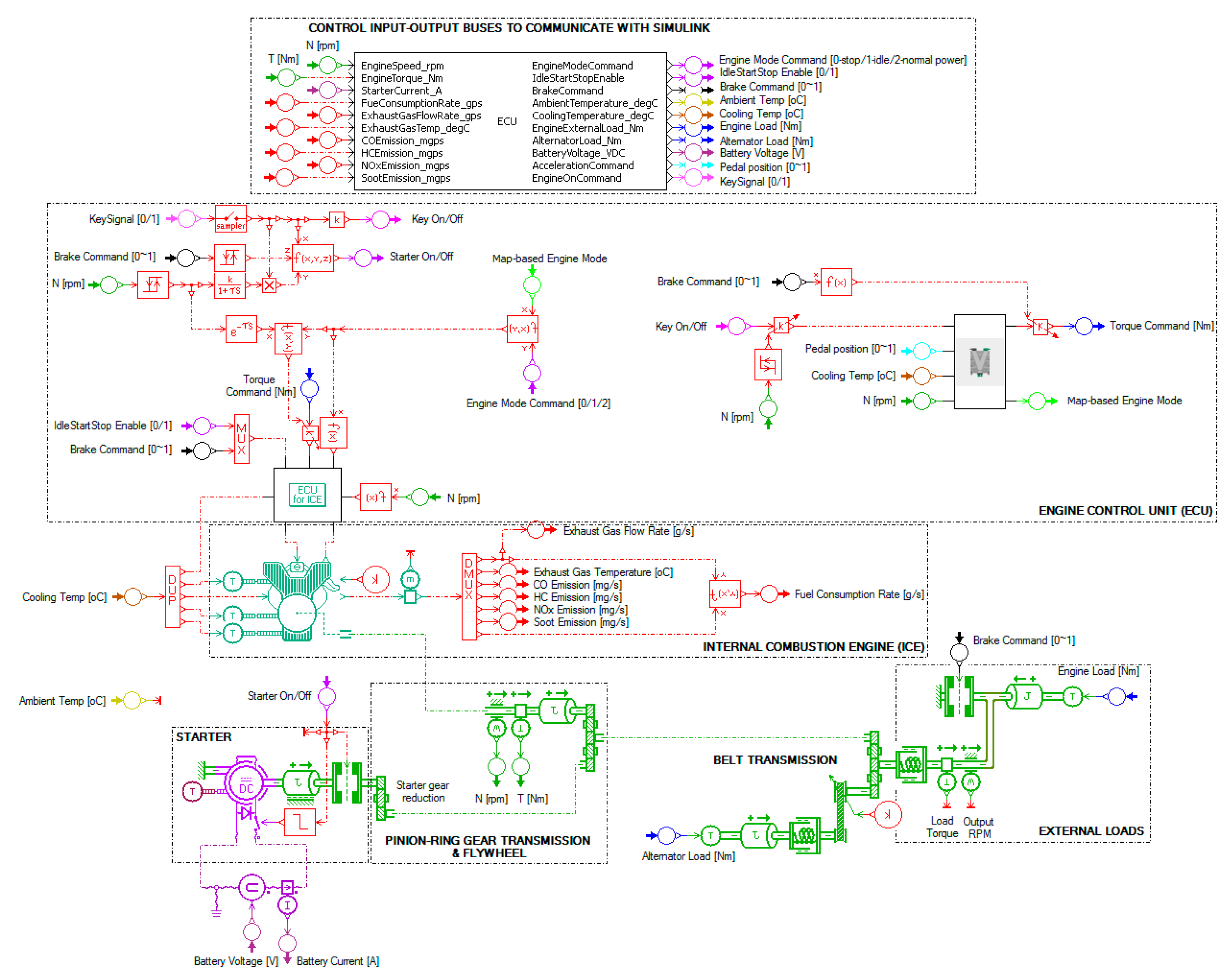
3.1. Component Models in AMESim

The set of sub-models built in AMESim and their connections is described in Figure 2. The figures shows that the AMESim model set comprises of ICE sub-model, starter sub-model, pinion-ring gear and belt transmissions’ sub-models, external loads’ sub-model, an engine control unit (ECU) to manage the ICE and starter operation, and an input/output (I/O) control interface to support the communication between AMESim and Simulink.

First, the engine is represented by a mean-value submodel in which the parameters are obtained from the transient ICE model presented in the prior study [8] and, torque map and brake specific fuel consumption map of the ICE are required. The model inputs are the ICE torque command and feedback speed, on/off/idle control signal, ambient temperature and coolant temperature. The model outputs are the generated ICE mechanical torque and pollutant emissions (CO₂, CO, HC, NO_x and soot). Second, the equivalent electrical circuit of a direct current machine with permanent excitation is used to model the starter motor in which the inputs are temperature, supply voltage and rotational speed, and the outputs are current and load torque. Third, the pinion-ring gear mechanism is modelled as a gear transmission connected to a controllable clutch while the flywheel is presented by a constant rotary load. Fourth, by assuming that there is no extension or damage of belt, the belt transmission sub-model is a set of a two-input-one-output rotary node, a gear transmission with fixed ratio and a rotary spring-damper. Fifth, external mechanical load at the engine output shaft is represented by a dynamic rotator of which the torque is given through the I/O control interface (see Figure 2). Other parameters for this AMESim model set, such as moments of inertia and friction coefficients, are obtained from the optimized powertrain model developed in [8]. This parameter set was derived using the nonlinear least-square-based parameter estimation method and the ICE cranking data of the target machine. Next, an engine control unit (ECU) is built with basic control logics to drive the ICE and starter sub-models:

• Engine torque control logics: base on the ICE speed command, current ICE speed and cooling temperature to compute the engine torque request;
• ECU’s input signals: the key On/Off event, calculated ICE torque request and brake command, ISSC enable, and engine mode command (will be defined in the next section);
• Basic engine operation logics: base on the defined modes to control the combustion process of the engine;
• Starter control logics: to drive the starter. In this typical powertrain, the starter is to crank the engine from zero speed to low idle speed. Once the engine reaches to its low idle speed, the injectors are activated to rise the engine speed to the high idle speed (ready to work) while the starter is disconnected from the powertrain and turned off.

At last, to perform the co-simulation with Simulink, the I/O control interface is created to receive the ICE and starter commands, and the simulated mechanical loads sent from the ISSC system and, conversely, to send the outputs of the AMESim model set back to the controller as well as the other component models in Simulink.

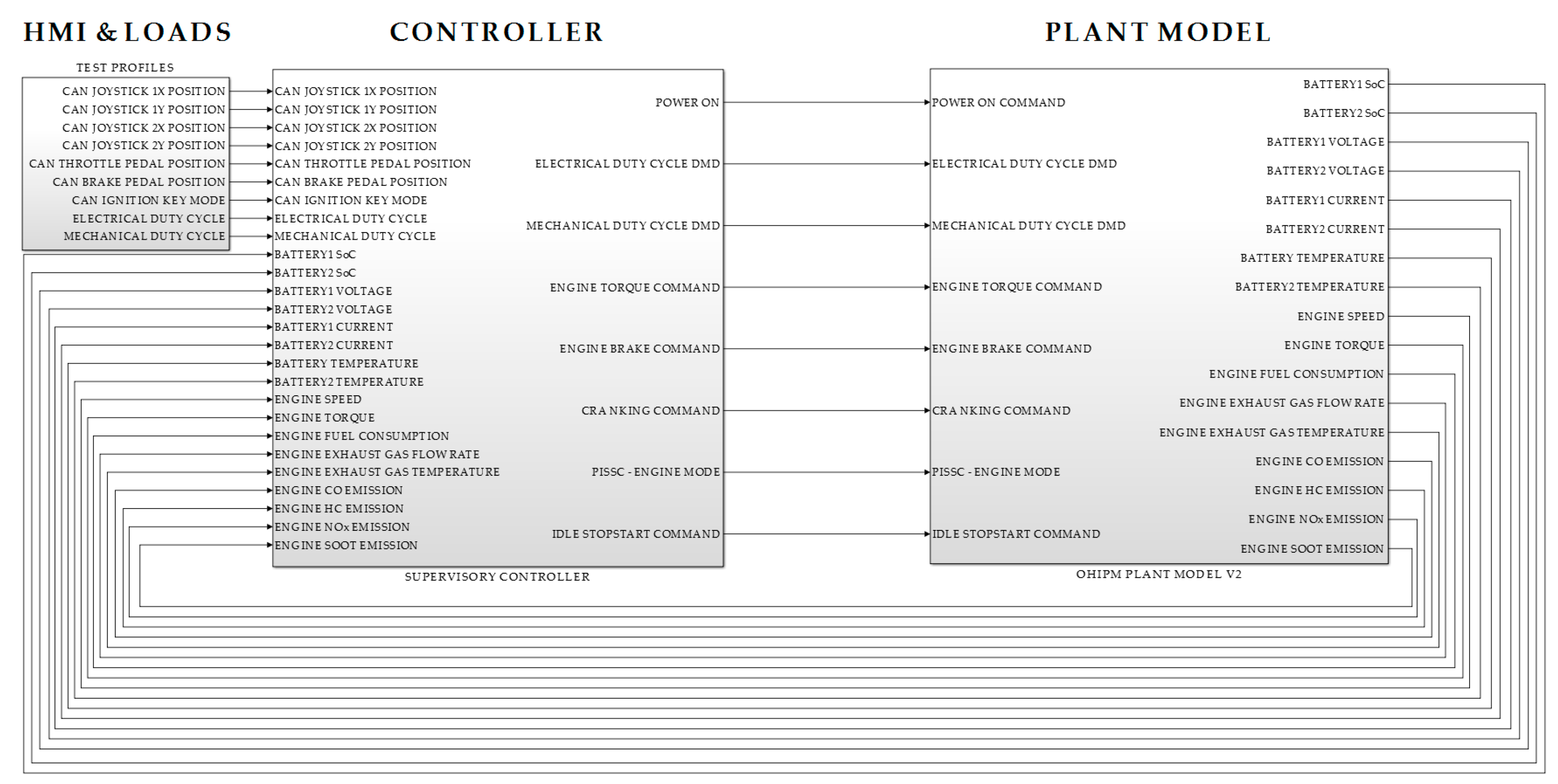
3.2. Component Models in Simulink

Next, the lead-acid battery, alternator and electrical load models are generated in Simulink using Simscape. The battery is represented by a two-RC-branch equivalent circuit model of which the parameters are derived based on the real test data and the curve fitting method [8]. The alternator model is created using look-up tables based on performance map of the actual alternator. Meanwhile, the electrical loads or total electricity demands for the excavator are represented by a variable resistor.

The AMESim model set is packaged as a black-box model and, then, converted into a Simulink S-function capable of working independently in Simulink environment without connecting to AMESim. As the result, the complete powertrain model is performed as shown in Figure 3.

4. Prediction-Based Idle-Stop-Start Control

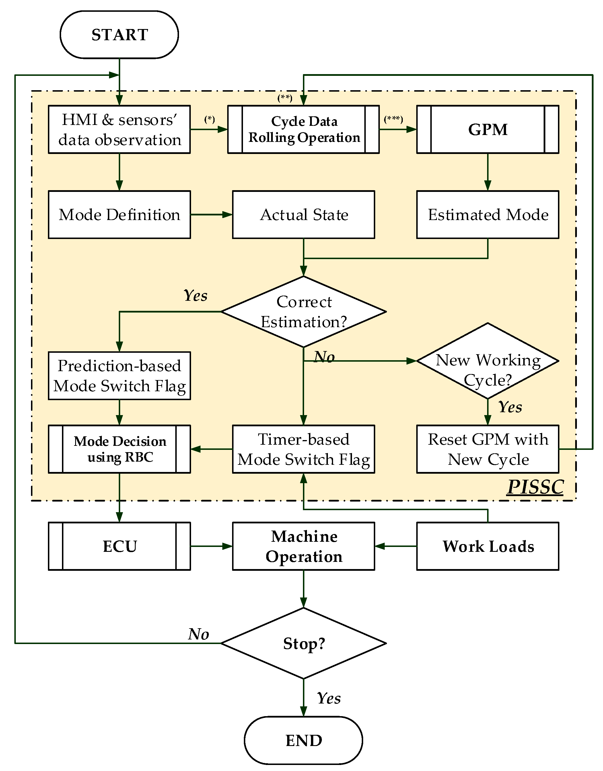
4.1. PISSC-Based Control Architecture

For a generic machine, the ICE control architecture integrated the PISSC scheme can be briefly represented in Figure 4. The operator interacts with the machine via a human-machine interface (HMI) module. From there, the operator is able to select flexibly between working modes, including normal power mode, PISSC mode and, possibly, other alternative modes. Due to the focus of this study on ISSC, only the engine operation according to main HMI commands, ICE states and workloads are taken into account and, therefore, other alternative modes are not considered.

Fundamentally during the operation, necessary machine information, such as, machine braking and acceleration commands from the pedals, and actuator commands from joysticks, are sent from the HMI to the engine speed controller. Synchronously, the current engine torque and speed are measured by proper sensors and fed back to this controller. By selecting the PISSC mode, these information are analysed to determine the most efficient mode for the ICE. The derived mode command is then transmitted to the ECU to drive the engine to the desired working point computed from the given engine commands.

For each machine type, a definition of torque-speed bands can be established to identify the ICE working modes. This definition is then used to design the PISSC. For the PISSC design, the following working modes are defined to manage the engine operation:

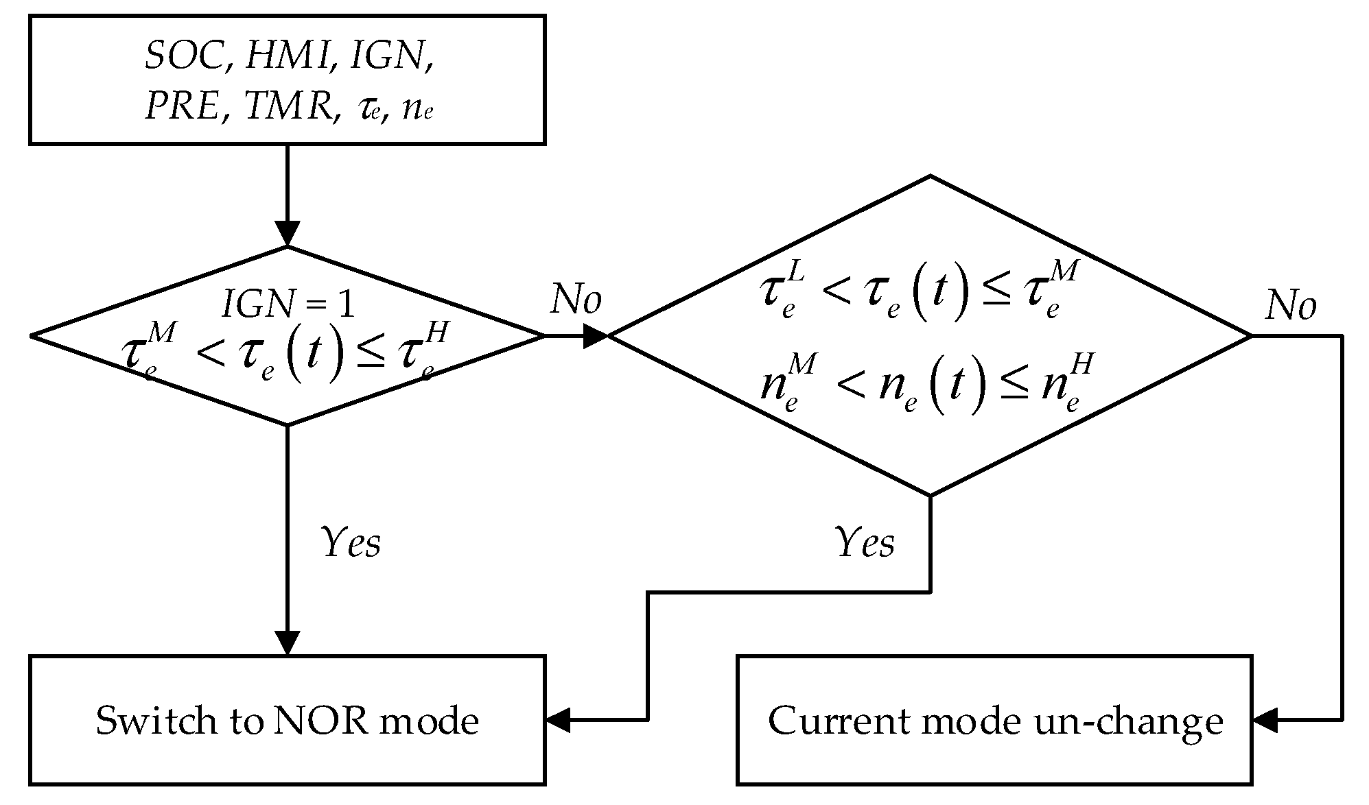
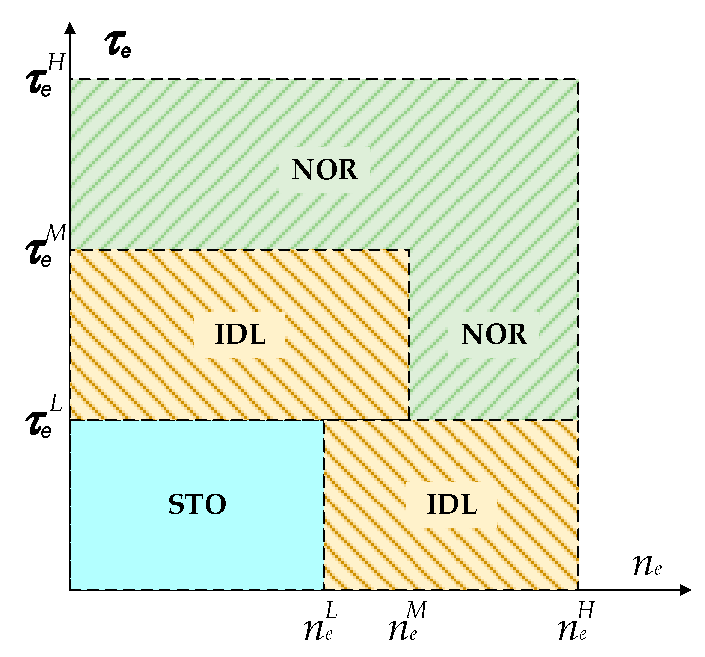
• NOR: normal mode, the machine is capable of working with full power capacity of the engine while the starter is off. This mode is used to drive the engine in the medium-high torque region or in the low-medium torque and medium-high speed region.
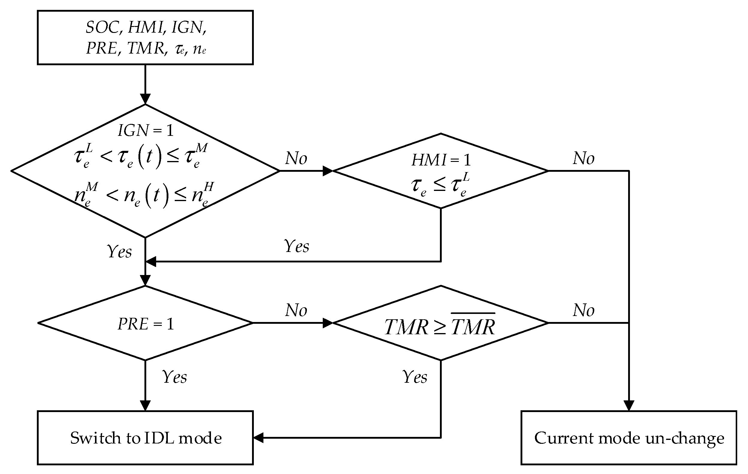
• IDL: idle mode, the engine does not work with its full power capacity by utilizing the cylinder deactivation control technology [14] while the starter is off. Therefore, this mode is used to drive the engine in the low-medium torque regions.
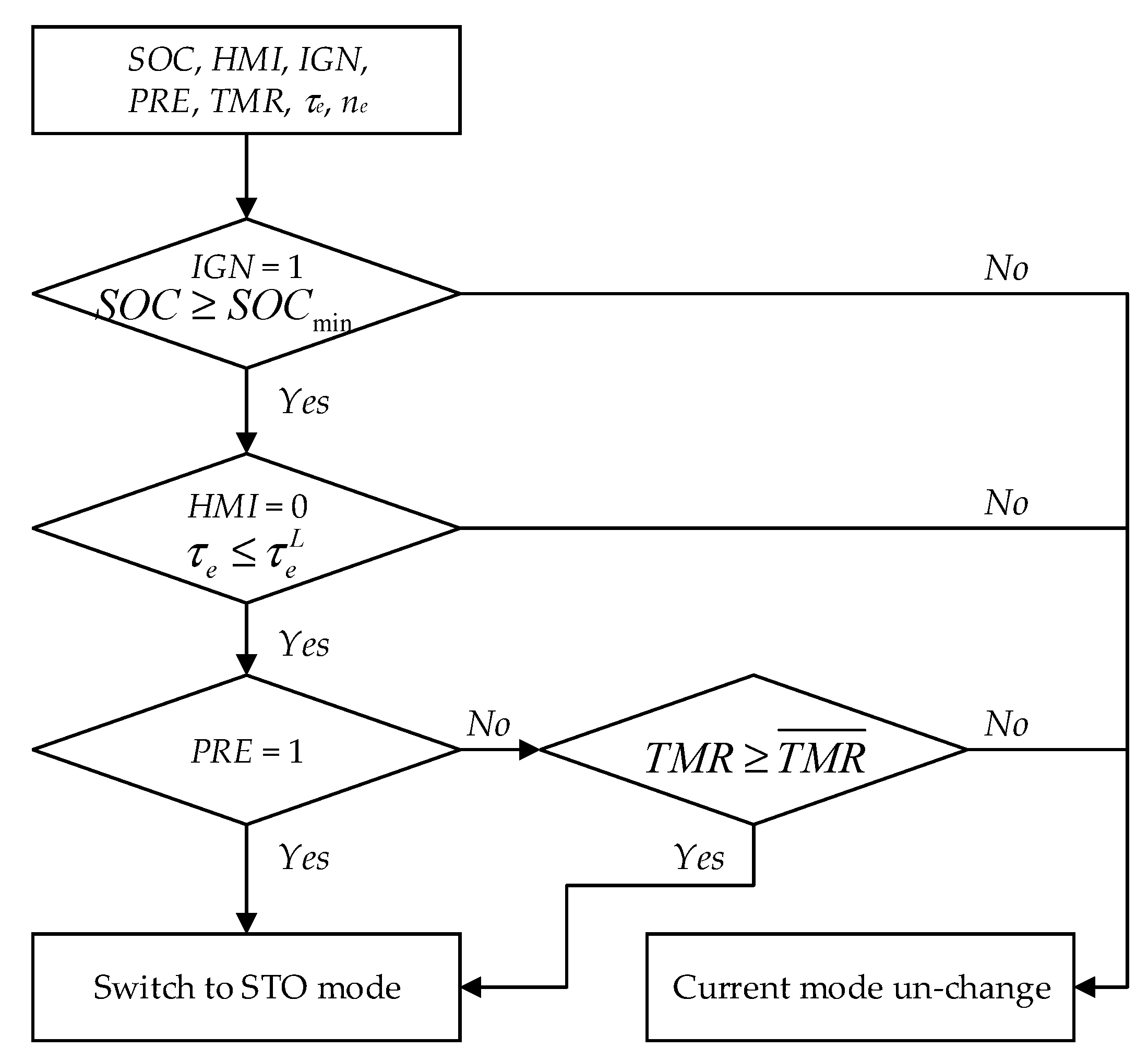
• STO: stop mode, the engine is shut down to save the fuel and the starter is also off. This mode is enabled when there is no command given from the HMI module, no external load and both the engine torque and speed are below the low torque and speed levels, respectively. The clutch C in Figure 1 is opened and, therefore, the ICE torque is only the sum of internal torque factors, including ICE torques, starter and alternator inertia torques and transmissions’ torque [8].
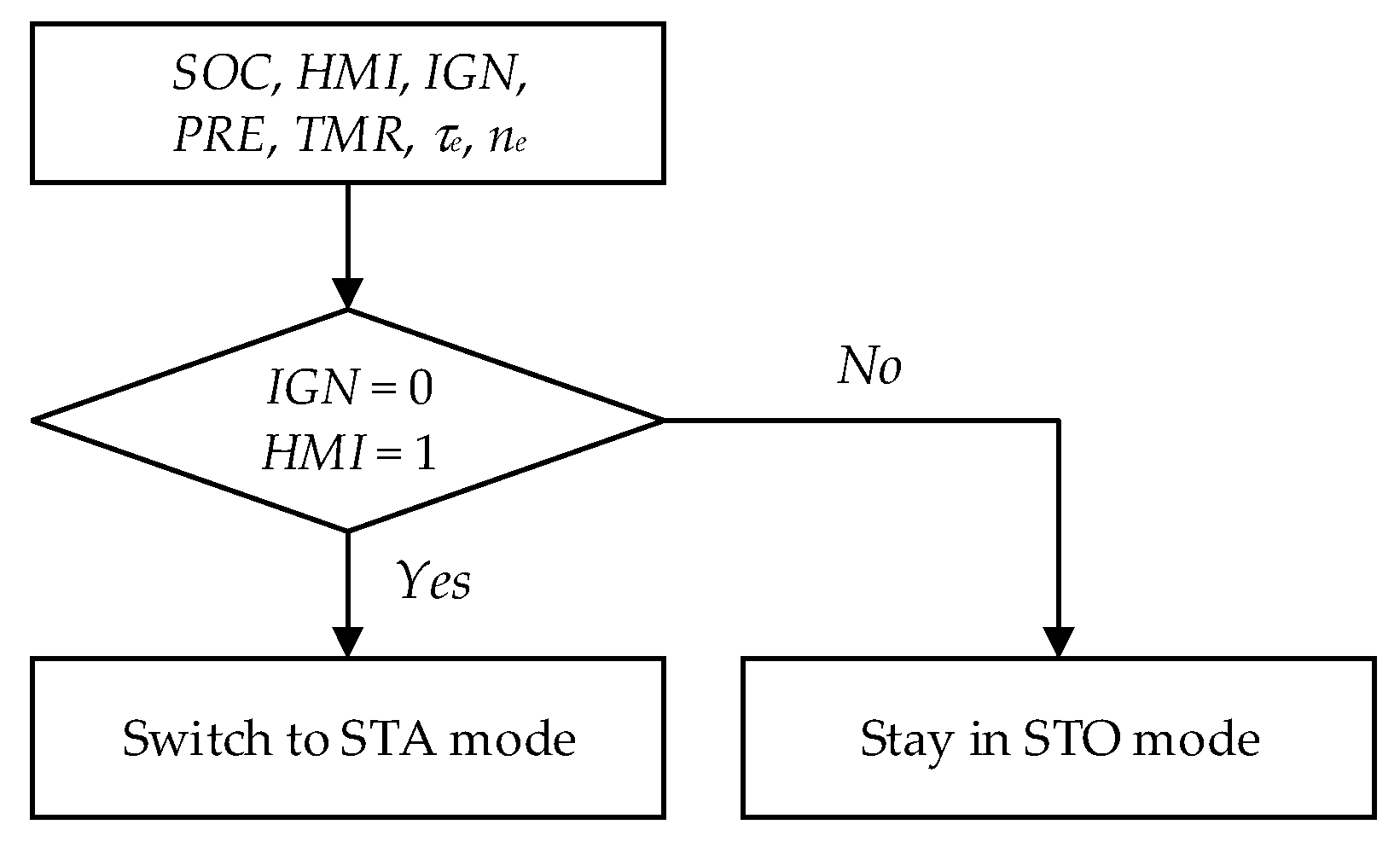
• STA: start mode, the engine is cranked from zero speed to its idle speed. The starter is firstly turned on to crank the ICE to a very low idle speed. At the low idle speed, the starter is switched off and the injector starts to inject fuel to continue to crank the engine to the desired idle speed.

Remark 1.

In order to design the PISSC, the following definitions are given:

• A machine cycle is a specific sequence of the ICE working modes (or machine stages) formed by the operator commands and workloads. Each stage can be identified using the feedback torque-speed and the ICE mode definition, and its duration is measured using the timer.
• A machine stage is recorded if its duration is not less than a pre-defined threshold value. This value is properly selected as 3 s based on the experts and machine/ICE dynamics to avoid a frequent ON/OFF commands on the engine. Each machine stage in a cycle then can be represented by a timestamp at which the stage begins.
• Two cycles having the same machine stage sequence are considered as two dissimilar cycles if, in one cycle, there exists a stage of which its duration is more than 10% difference compared to that of the corresponding stage in the other one.

Next, a working flow diagram of the PISSC module to control the engine speed is designed as shown in Figure 5. During the operation, the signals from the HMI and ICE sensors (torque and speed) are acquired to identify the current ICE working mode in real-time based on the torque-speed band definition (or mode definition). At the same time, these information are used to identify online any repeated working cycles using the cycle data rolling operation module and Remark 1. Once the identified cycle is recorded that it is repeatedly and continuously operated for a few times, the GPM module is enabled to estimate the coming engine mode when a new machine stage corresponding to a new ICE mode (compared to the current mode) is detected. This estimated engine mode is compared with the actual machine state to determine the prediction accuracy. Synchronously, a timer is activated to measure duration of the new ICE mode. The correct prediction result and the timer-based mode decision are both input to a rule-based controller (RBC) to make a final decision on mode switching. This decision is then sent to the ECU and, subsequently, the ECU can drives the engine in its highest fuel efficiency zone without sacrificing the machine performance.

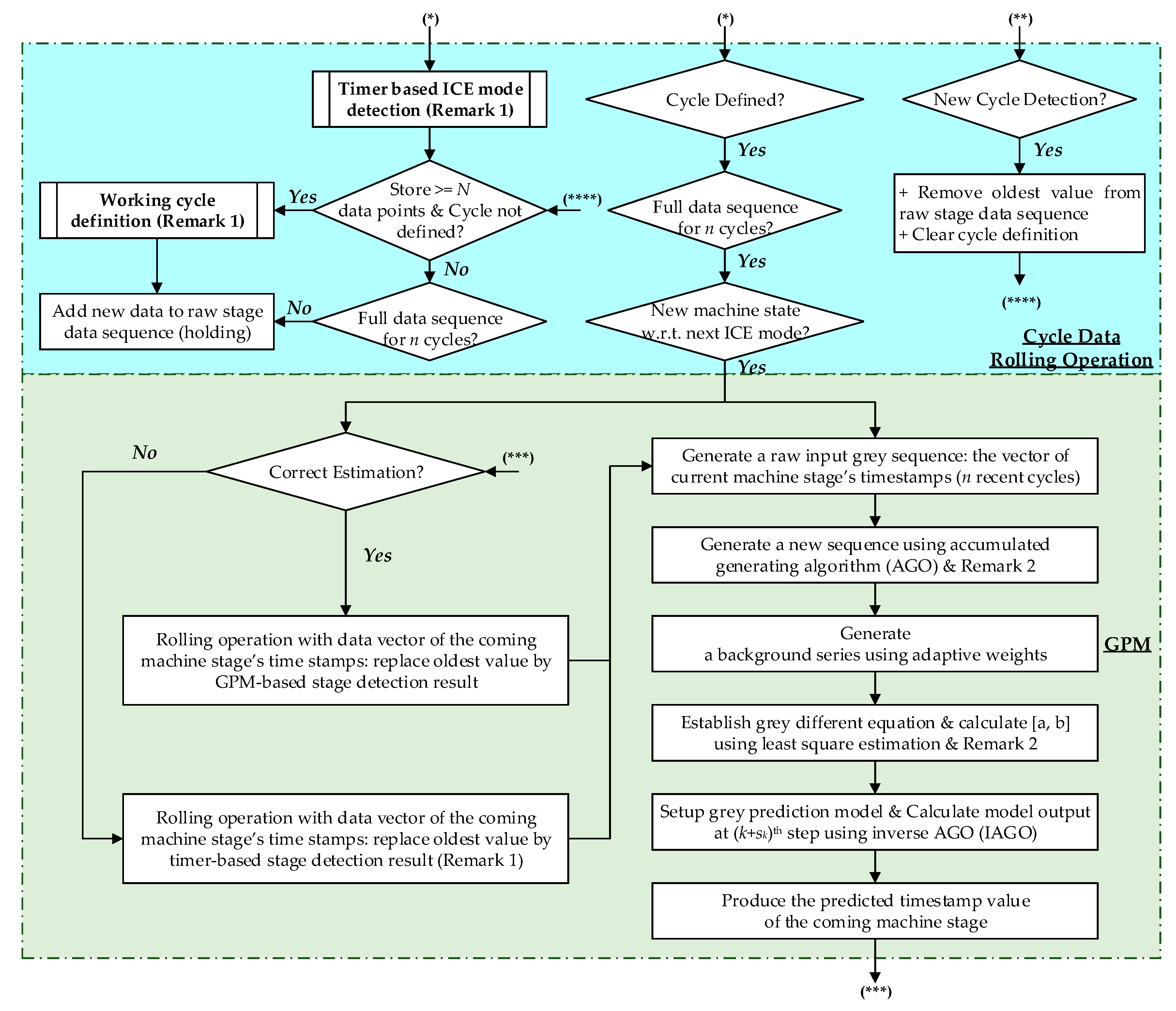
4.2. Cycle Data Rolling Operation

In order to manage the historical data necessary for the prediction using the GPM, the cycle data rolling operation module is built as shown in Figure 5 and the top blocks in Figure 6. This module includes three main functions: working cycle identification, raw data preparation for the GPM and GPM activation control.

The timer is firstly used to determine working cycles. This timer is reset and activated when a new machine stage is detected from the machine information (the HMI and torque-speed sensors’ signals). In order to detect a repeatable cycle, a minimum number of machine stages, N, needs to be recorded. Based on the number of working modes and working behavior of the machine, this number is assigned to 20 (N = 20). By using Remark 1, the working cycle can be then identified by a simple iterative searching algorithm:

• Step 1: start the search with an initial number of stages per cycle (S), S₀ = 2 which means the first 02 consecutive stages;
• Step 2: Check the repeatability of this stage sequence: If YES, check: the time differences of the cycle’s stages are equal or less than 10%
  • + If YES, stop the search and make a decision of the machine cycle;
  • Else, go to Step 3;
  Else, go to Step 3;
• Step 3: If S less than N, increase the number of stages per cycle: S = S + 1; Else, delete the oldest value from the recorded stage vector and stop the search.

One a periodic cycle is determined, the recorded machine stages are re-arranged in to a matrix form of cycle number, stages’ indices and timestamps within a cycle. Based on the grey prediction theory (introduced in the next section), a vector with minimum number of historical time series stage data (denoted as n corresponding to n continuously repeated cycles) is required to perform the prediction of a coming machine stage. As a result, the prediction is only enabled when the recorded stage matrix contains historical data of n cycles.

During the operation of cycle (n + 1)th, a detection of any new machine stage which is matched with the defined stage sequence of the cycle, the most recent time series data vector of this stage (with n elements) is sent to the GPM. On the contrary, a new machine stage which is different from the defined stage sequence exists, the cycle definition is reset. The recorded matrix is again converted in to the vector type in which the oldest element is replaced by the new value using the first-in-first-out rule. Consequently, the iterative searching algorithm is executed again to find out a new cycle definition before re-activating the prediction.

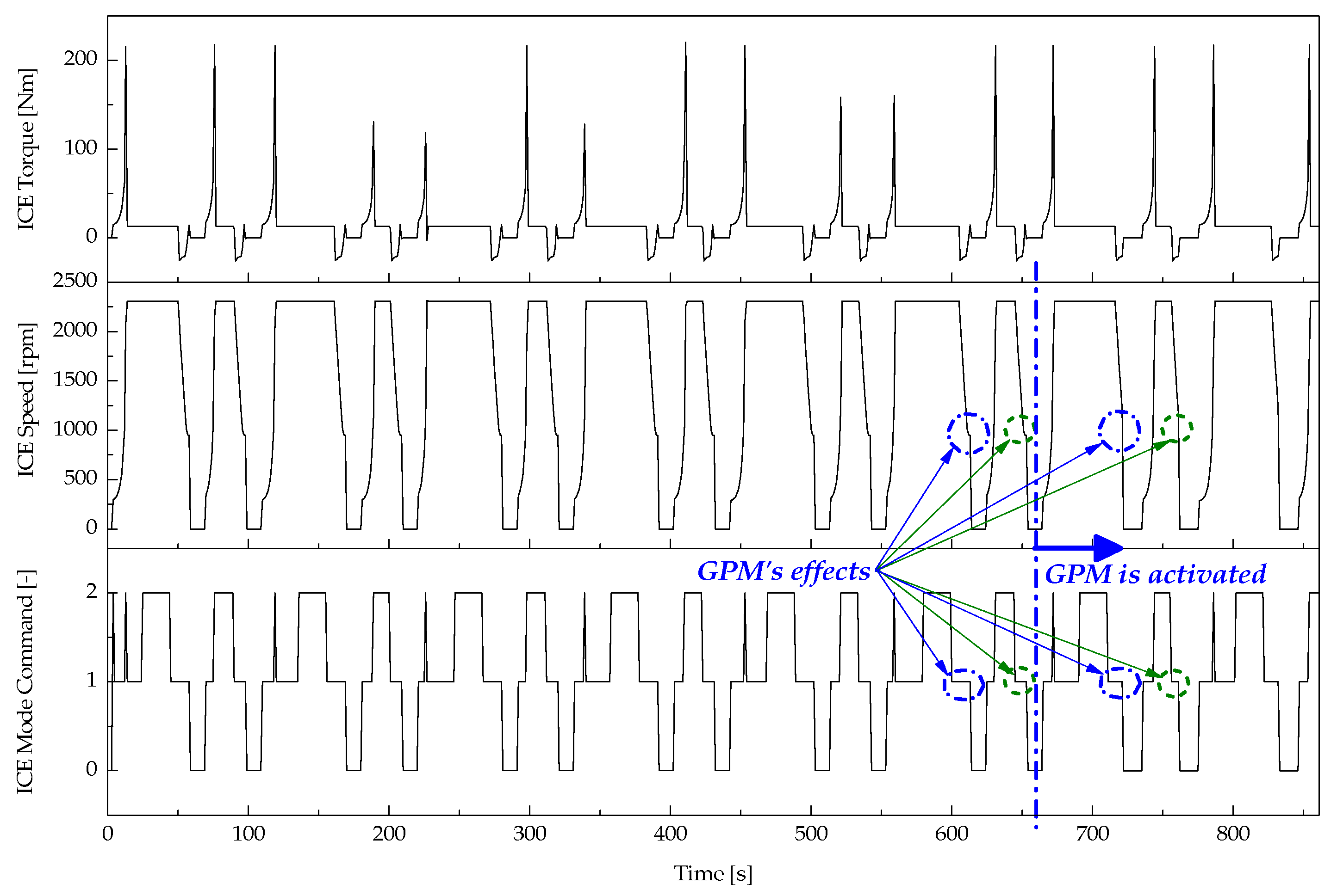
4.3. Grey Prediction Model

The grey technique has rapidly become a well-known estimation tool to deal with systems with partially unknown parameters [15]. GM(1,1) (single-variable first-order grey model) is the most popular grey model which has been successfully applied to a wide variety of applications ranging from economics to engineering [16,17,18,19,20]. However, a typical GM(1,1) is only capable of dealing with non-negative data sequences satisfying the condition of a grey data sequence, including quasi-smooth and quasi-exponential checking conditions [16]. To overcome this limitation, in this study, the first order grey prediction model GPM is developed based on the authors’ previous work [16,18] to estimate the ICE modes. By the use of two additive factors, the prediction can be performed with any random time-series signal. Because the GPM is activated only when existing a new machine stage, only one GPM with one variable (timestamp of the coming stage) is required to minimize the computational cost while ensuring the PISSC’s functions. The flow diagram of this GPM in combination with the cycle data rolling operation module is described in Figure 6.

From this figure, the procedure to predict the coming machine stage can be expressed as the following steps:

Step 1:

Create an input grey sequence $y^{\left(0\right)}$ when the GPM is activated:

Take a vector of the machine stage’s timestamps of n recent cycles:

$$\left\{y_{raw}(t_{O1}),y_{raw}(t_{O2}),...,y_{raw}(t_{On})\right\};n\ge 5$$

(1)

Create a new series from (1) using Remark 2:

$$\begin{array}{l}{Y}^{\left(0\right)}=\left\{y^{\left(0\right)}\left(t_1\right),y^{\left(0\right)}\left(t_2\right),...,y^{\left(0\right)}\left(t_n\right)\right\}>0;n\ge 5\\ y^{\left(0\right)}\left(t_k\right)=y_{raw}^{}\left(t_k\right)+c_1+c_2;k=1,...,n\end{array}$$

(2)

Remark 2.

By adding two non-negative smart additive factors c₁ and c₂ derived by Theorem 1 in [16], the sequence (1). becomes (2) and satisfies all the conditions to establish a grey model: positive sequence, quasi-smooth and quasi-exponential conditions.

Step 2:

Generate a new series Y⁽¹⁾ from Y⁽⁰⁾ using the accumulated generating algorithm (AGO):

$$\begin{array}{l}{y}^{\left(1\right)}\left(k\right)={\displaystyle {\sum }_{i=1}^k{y}^{\left(0\right)}\left(t_i\right)}\times \Delta t_i,k=1,2,...,n\\ ={\displaystyle {\sum }_{i=1}^k\left(y_{raw}\left(t_i\right)+c_1+c_2\right)}\times \Delta t_i\end{array}$$

(3)

Step 3:

Generate a background series Z⁽¹⁾ from Y⁽¹⁾ using the mean algorithm as

$$z^{\left(1\right)}\left(t_k\right)=0.5y^{\left(1\right)}\left(t_k\right)+0.5y^{\left(1\right)}\left(t_{k-1}\right);k=2,...,n$$

(4)

Step 4:

Establish the GPM first-order differential equation

$$y^{\left(0\right)}\left(t_k\right)+a{z}^{\left(1\right)}\left(t_k\right)=b$$

(5)

Remark 3.

By employing the least square estimation [15], the prediction of the object y using the GPM model is optimized if the parameters a and b in (5) satisfy (6):

$${\widehat{\beta }}_{ab}={\left[\begin{array}{cc}\widehat{a}& \widehat{b}\end{array}\right]}^T={(B^{T}B)}^{-1}{B}^{T}Y$$

(6)

where:

$$B=\left[\begin{array}{cc}-z^{\left(1\right)}\left(t_2\right)& 1\\ -z^{\left(1\right)}\left(t_3\right)& 1\\ ⋮& ⋮\\ -z^{\left(1\right)}\left(t_n\right)& 1\end{array}\right],Y=\left[\begin{array}{c}{y}^{\left(0\right)}\left(t_2\right)\\ y^{\left(0\right)}\left(t_3\right)\\ ⋮\\ y^{\left(0\right)}\left(t_n\right)\end{array}\right]$$

Step 5:

Perform the GPM prediction:

$${\widehat{y}}^{\left(0\right)}\left(t_k\right)=\frac{\widehat{b}-\widehat{a}\left(w_k^1+w_k^2\right)y^{\left(1\right)}\left(t_{k-1}\right)}{1+w_k^1\widehat{a}\Delta t_k}$$

(7)

Step 6:

Compute the predicted value of ${\widehat{y}}_{raw}$ at step (k + s_k)^th using (7) and the inverse AGO (IAGO):

$${\widehat{y}}_{raw}\left(t_{k+s_k}\right)={\widehat{y}}^{\left(0\right)}\left(t_{k+s_k}\right)-c_1-c_2$$

(8)

where s_k is the prediction step size and selected as a unit in this case.

Step 7:

Check the prediction accuracy by comparing to the actual timestamp at which the machine stage is firstly detected:

(1)

De-activate the GPM and send the prediction result to the RBC for a mode decision;

(2)

If the prediction result is acceptable, with 5% accuracy, the machine stage data vector is updated with the estimated value using the rolling algorithm; Otherwise, the machine stage data vector is updated with the result of the timer-based ICE mode detection using the rolling algorithm;

(3)

Update fully the recorded stage matrix once the machine completes a working cycle using the rolling algorithm.

4.4. Rule-Based Controller Design for ICE Mode Decision

Based on the machine information and the outputs from the GPM and timer, the RBC, is designed to switch the ICE mode between NOR, IDL, STO and STA. Let’s define the following variables:

• ${\tau }_e\mathrm{and}{n}_e$ are the engine torque and speed, respectively. By using the actual torque-speed performance map of each specific machine, three torque and speed levels, high, medium and low, are in turn selected as: ${\tau }_e^H,{\tau }_e^M,{\tau }_e^L\mathrm{and}{n}_e^H,n_e^M,n_e^L$ to determine the ICE modes.
• HMI (HMI flag) is a variable which is unit if there exists at least a signal sent from the HMI module, and is zero vice versa.
• TMR is value of the timer which counts number of continuous states of the engine which are within the same working mode difference from the current mode. This TMR is reset once having a new series of engine states or a new engine mode selected. $\overline{TMR}$ is the pre-defined threshold value for TMR, $\overline{TMR}=3$.
• PRE is a variable representing a correct estimation of the GPM (if the estimation error is within a pre-defined acceptable range). Then, PRE = 1 if correct and PRE = 0 if not correct.
• IGN is a variable representing the engine state, IGN = 1 if ICE is on and IGN = 0 if ICE is off.
• SOC is the battery state of charge representing the energy remained in the battery (in percentage). In order to enable stop-start operation, this SOC should be greater than a minimum level SOC_min which allows the starter can crank the engine when STA mode is enabled. In this case, SOC_min is set to 70%.

Next, based on the ICE modes’ properties (Section 4.1) and torque-speed band, the ICE working regions are defined as displayed in Figure 7.

By updating all the declared variables and ICE working regions, the rules are then established for the RBC as follows:

• Rule for NOR mode: when the ICE is running (IGN = 1), if the ICE torque and speed satisfy: ${\tau }_e^M<{\tau }_e\left(t\right)\le {\tau }_e^H$ or (${\tau }_e^L<{\tau }_e\left(t\right)\le {\tau }_e^M$ and $n_e^M<n_e\left(t\right)\le n_e^H$), the ICE is shifted to NOR mode; otherwise, it continues to stay in the current mode. This logic is demonstrated in Figure 8.

• Rule for IDL mode: when the ICE is running (IGN = 1), if the ICE torque and speed satisfy: (${\tau }_e^L<{\tau }_e\left(t\right)\le {\tau }_e^M$ and $n_e\left(t\right)\le n_e^M$) or (${\tau }_e\left(t\right)\le {\tau }_e^L$ and $HMI=1$), one has:

  (1)

  + The outputs from the GPM and timer are considered; if PRE = 1 or $TMR>\overline{TMR}$, the ICE is shifted to IDL mode;

  (2)

  + Otherwise, it continues to stay in the current mode as described in Figure 9.

• Rule for STO mode: when the ICE is running (IGN = 1) and battery is healthy $(SOC\ge SO{C}_{\min })$, if the ICE torque satisfies ${\tau }_e\left(t\right)\le {\tau }_e^L$ and there is no HMI signal $(HMI=0)$, one has:

  (1)

  + The outputs from the GPM and timer are considered; if PRE = 1 or $TMR>\overline{TMR}$, the ICE is shifted to STO mode;

  (2)

  + Otherwise, it continues to stay in the current mode as described in Figure 10.

• Rule for STA mode: when the ICE is stopped (IGN = 0), if there exists any signal sent from HMI (HMI = 1), the ICE is shifted to STA mode; otherwise, it continues to stay in the STO mode. This logic is demonstrated in Figure 11.

5. Case Study and Simulation Results

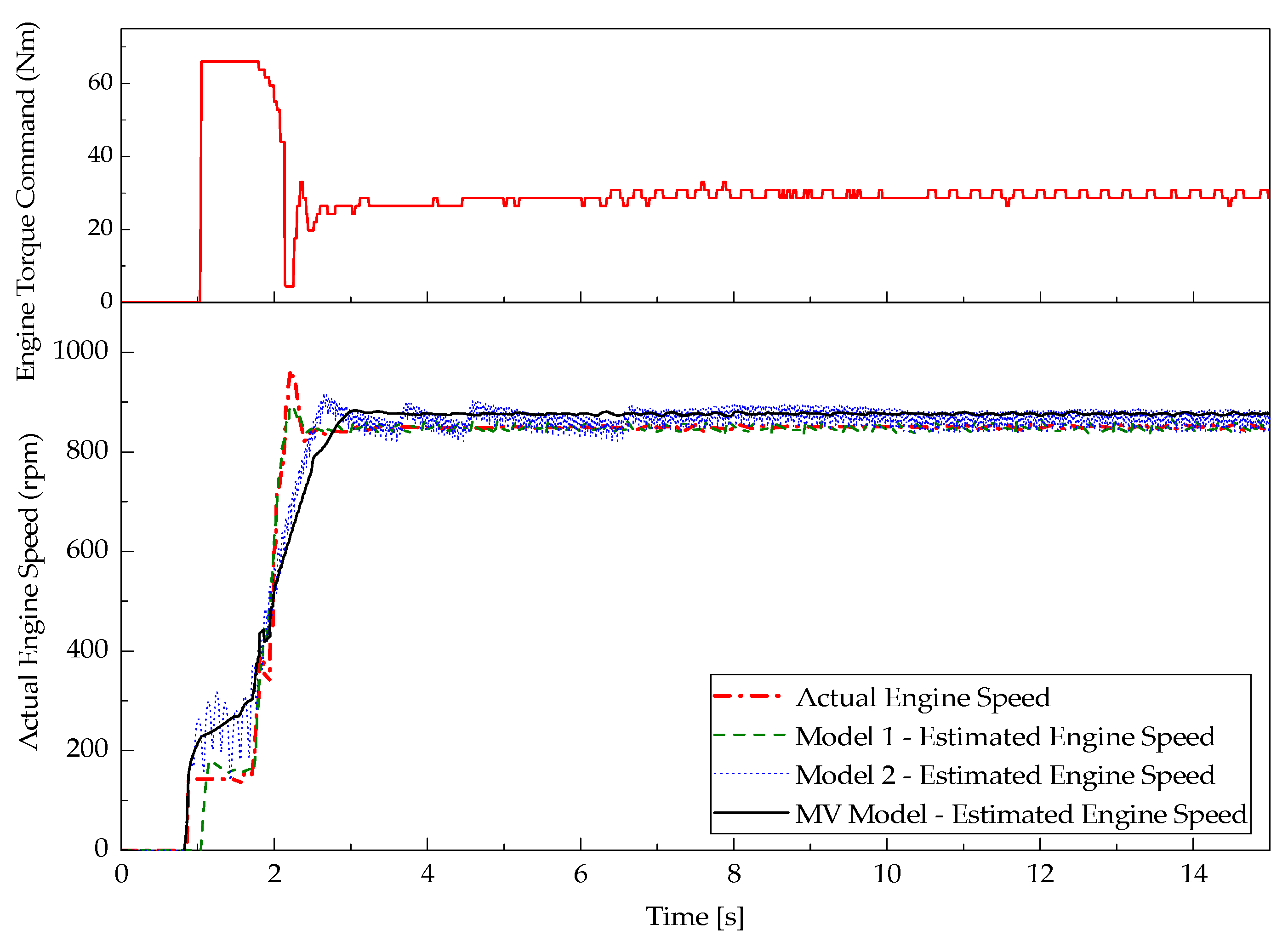
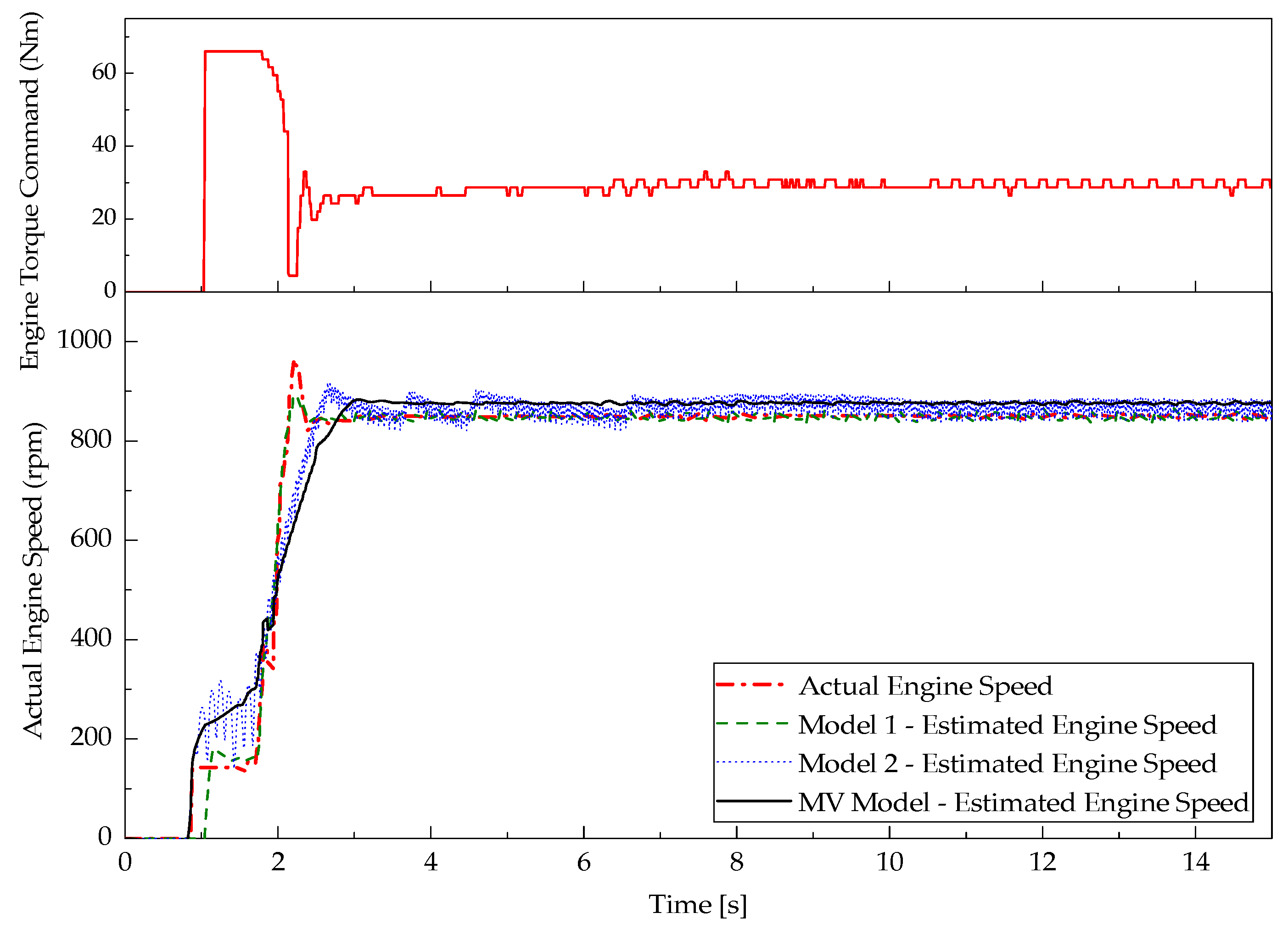
5.1. Powertrain Model Validation

Simulations have been firstly carried out to validate the applicability of the powertrain model presented in Section 3. A comparative study between this mean-value model (tagged as the MV Model) and the two optimal transient models developed in [8], the mathematical model—Model 1 and the high fidelity AMESim model—Model 2, was selected for the simulation of ICE cranking process to crank the engine from zero rpm to low idle speed of 850 rpm. Two time-series data sets of the ICE torque command input and the ICE speed response observed from two real cranking experiments on the target machine [8] were used to assess the modelling accuracy.

For the simulations, the actual ICE torque command input measured at the ECU was directly input to the ECU models to simulate the ICE response. The comparison of simulation results are then demonstrated in Figure 12 and Figure 13. The results indicate that both the models could estimate the ICE speed profiles. Although, in both the tests, the best performance was achieved by using Model 1, this model is complex and lacks any capability to estimate the ICE fuel consumption and emissions. The modelling accuracies of Model 2 and MV Model were quite similar as the MV Model was constructed using the optimal parameter set of the Model 2 (Section 3). However, by using the mean-value modelling approach, the MV Model could perform the simulation with the fastest simulation speed compared to the Model 1 and Model 2. In addition, the MV Model could provide all necessary information to evaluate the machine performance. Therefore, this model is suitable for the aims of this study.

5.2. Excavator Tracking Control Simulations

5.2.1. Test Case Definition and Simulation Setup

In this section, simulations of the excavator representing by the selected MV Model have been carried out to evaluate the performance of the proposed PISSC approach. A working cycle consisting of all the ICE modes defined in the previous section is necessary to perform the investigation. To generate this cycle, main HMI signals and environment conditions are chosen and defined in

Table 4. Definition of HMI signals and environment conditions.

Signal	Description	Range	Unit	Actual Range & [Actual Unit]
Key	Key even by operator with three position: Off (0)-On (1)-Ignition (2)	0-1-2 (Integer)	-	0-1-2 [-]
AP	Acceleration pedal command given by operator	0~100 (Proportional)	%	0~100 [-]
JX1	Joystick 1—X command	0~100 (Proportional)	%	0~100 [-]
JY1	Joystick 1—Y command	0~100 (Proportional)	%	0~100 [-]
JX2	Joystick 2—X command	0~100 (Proportional)	%	0~100 [-]
JY2	Joystick 2—Y command	0~100 (Proportional)	%	0~100 [-]
BP	Brake pedal command given by operator	0~100 (Proportional)	%	0~100 [-]
Elec Load	Equivalent electrical loads of machine	0~100 (Proportional)	%	0~Max electrical load [W]
Mech Load	Equivalent mechanical load torque on ICE shaft	0~100 (Proportional)	%	0~Max simulated load torque [Nm]
Env Temp	Environment temperature	20 (Constant)	°C	20 [°C]
Cool Temp	Coolant temperature	60 (Constant)	°C	60 [°C]

. Here, the two 2-axis joysticks (denoted as JX₁, JY₁, JX₂ and JY₂) to control the hydraulic actuators of the machine while the acceleration and brake pedals to control the machine traction.

By using the definition of HMI signals and environment conditions, a working cycle is generated in

Table 5. A simulated working cycle for heavy excavator.

Phase No.	Phase Time Stamp [s]	Machine Key	Mech Load 1 M [%]	Elec Load 2 E [%]	JX1 [%]	JX2 [%]	JY1 [%]	JY2 [%]	AP [%]	BP [%]
1	0.01	0	0	0	0	0	0	0	0	0
2	3	1	0	100	0	0	0	0	0	0
3	4	2	0	100	0	0	0	0	0	0
4	5	1	50	100	100	0	100	0	0	50
5	10	1	50	100	0	100	0	100	0	50
6	15	1	50	100	100	100	0	0	0	50
7	20	1	50	100	0	0	100	100	0	50
8	25	1	50	100	100	100	0	0	0	50
9	30	1	100	100	0	0	0	0	100	100
10	40	1	100	100	20	20	0	0	50	100
11	45	1	50	100	20	20	0	0	0	50
12	50	1	0	100	0	0	0	0	0	0
13	70	1	20	100	100	100	0	0	0	20
14	75	1	20	100	20	20	0	0	100	20
15	85	1	20	100	0	0	0	0	50	20
16	90	1	0	100	0	0	0	0	0	0
17	110	1	20	100	100	0	0	100	0	20
18	115	1	50	100	0	100	100	0	0	50

¹ Simulated load applied to ICE shaft = ICE internal load (inertia and frictions come from the model) + M × A pre-defined external load/100; ² Simulated electrical load = E × A predefined electrical load/100.

which is based on experts experience about common activities of excavator. Wherein, 18 machine phases with different HMI commands and different mechanical/electrical loads are given in a time series sequence. For each simulation, the first three phases is only executed one time to represent the operator action to turn on the machine first time by using the machine key. Next, the other phases are repeatedly operated to simulate a test case with the cyclic operation in which phase 18th of cycle nth is linked to phased 4th of cycle (n + 1)th. The equivalent mechanical and electrical loads are transferred directly to the plant model to simulate the working conditions. In this study, the effects of temperature have not been considered. Hence, the environment and coolant temperature are kept as constants at 20 °C and 60 °C, respectively.

The full excavator simulation system is then built in Simulink as demonstrated in Figure 14. Herein, the ‘PLANT MODEL’ block is the complete powertrain model (Figure 3) while the ‘CONTROLLER’ block contains two comparative ICE controllers:

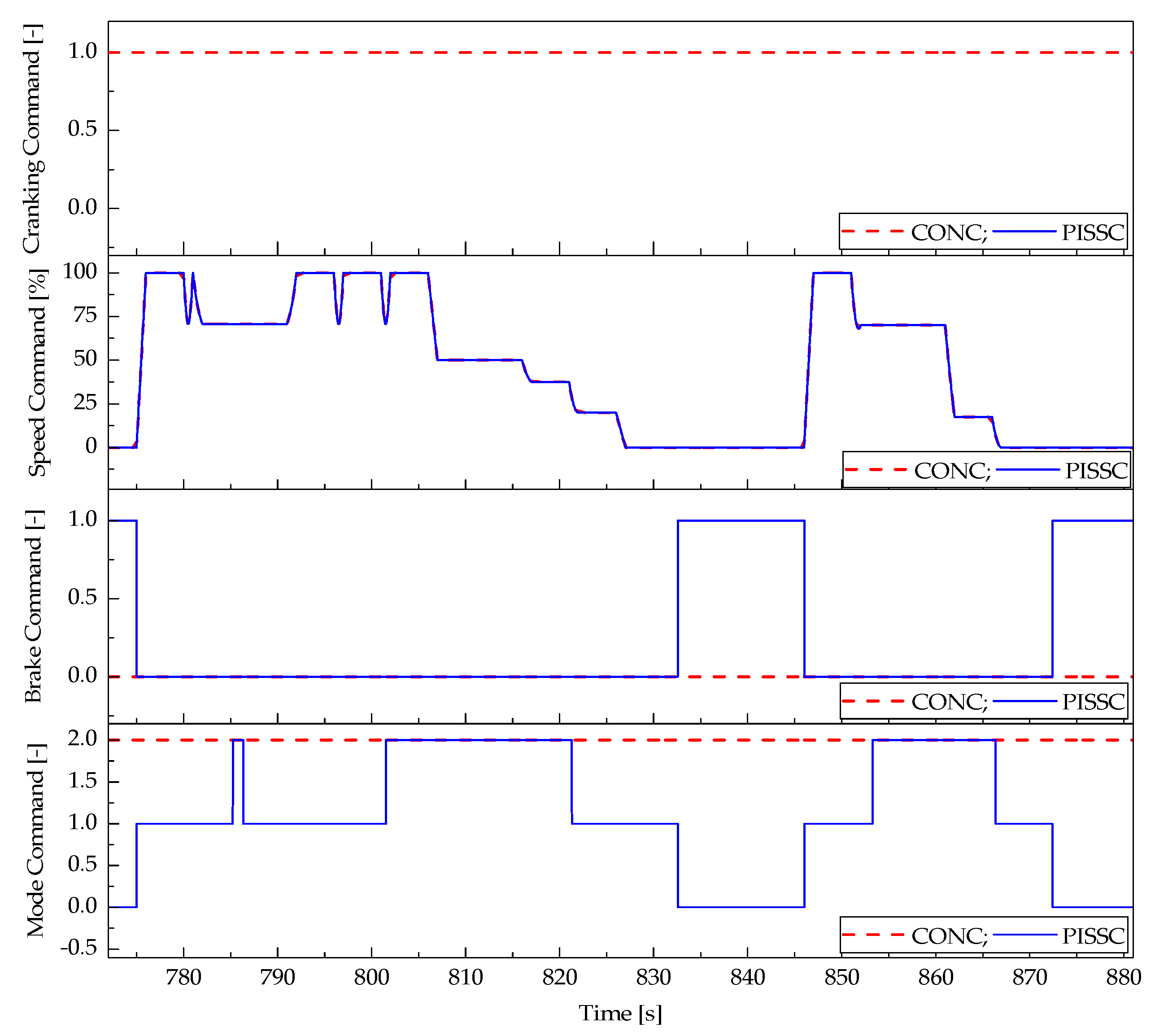
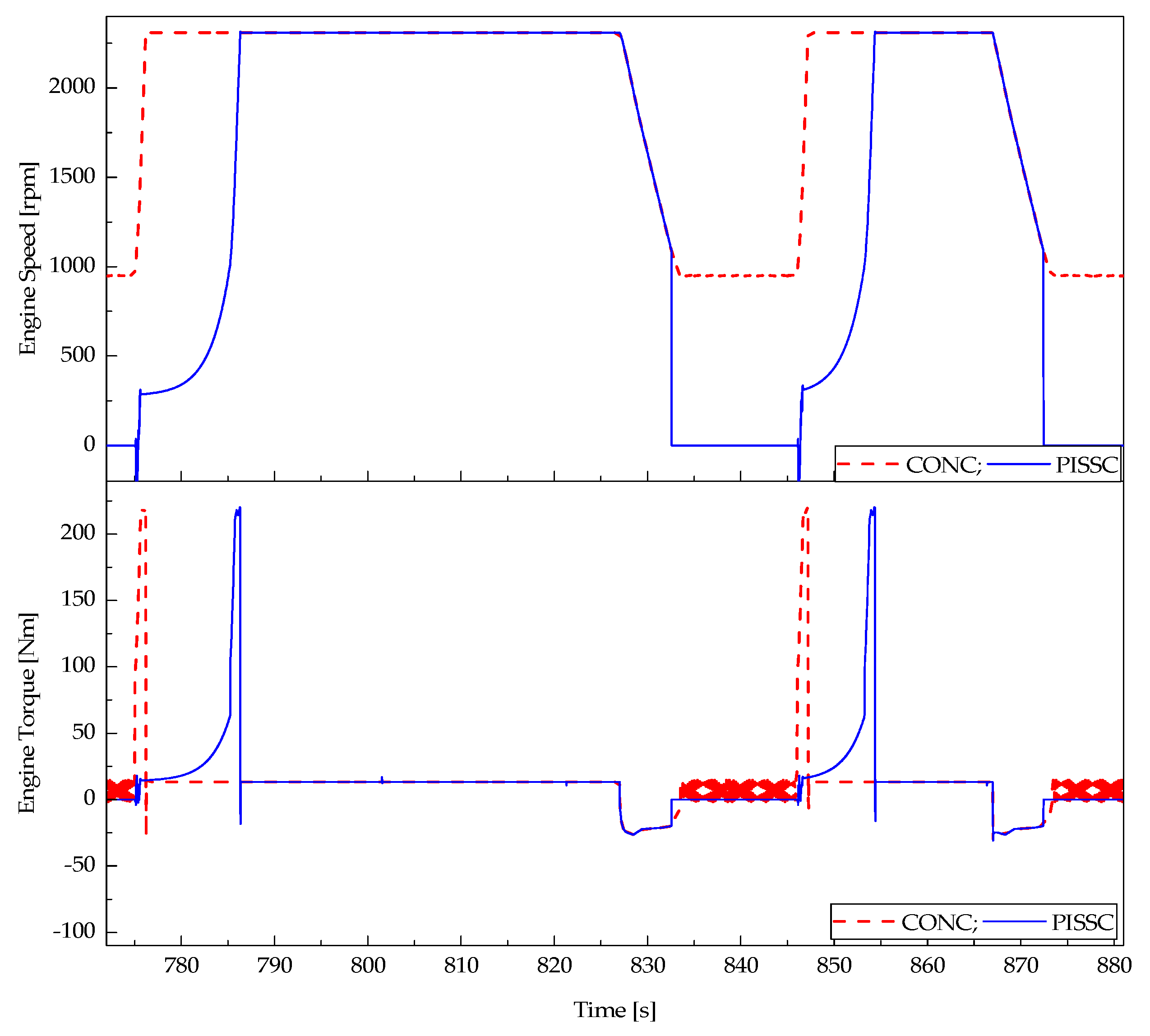
• Conventional controller, tagged as CONC: contains only the simple engine speed control logics of the traditional excavator without idle-stop-start function. Once the machine is running under the simulated loading condition using the equivalent load torque, the engine is always on, and its output power is driven by the HMI commands.
• Proposed controller, PISSC, developed in Section 4: contains not only the logics of the CONC but also prediction-based ISS function. Once the machine is running, the ICE output power is driven by the HMI commands while the ICE mode is controlled by the ISS function to maximize the fuel efficiency of the ICE. The ICE mode prediction is inactive during the first n working cycles (Section 4.3, selected as n = 6) in order to observe enough historical timestamp data to support the prediction.
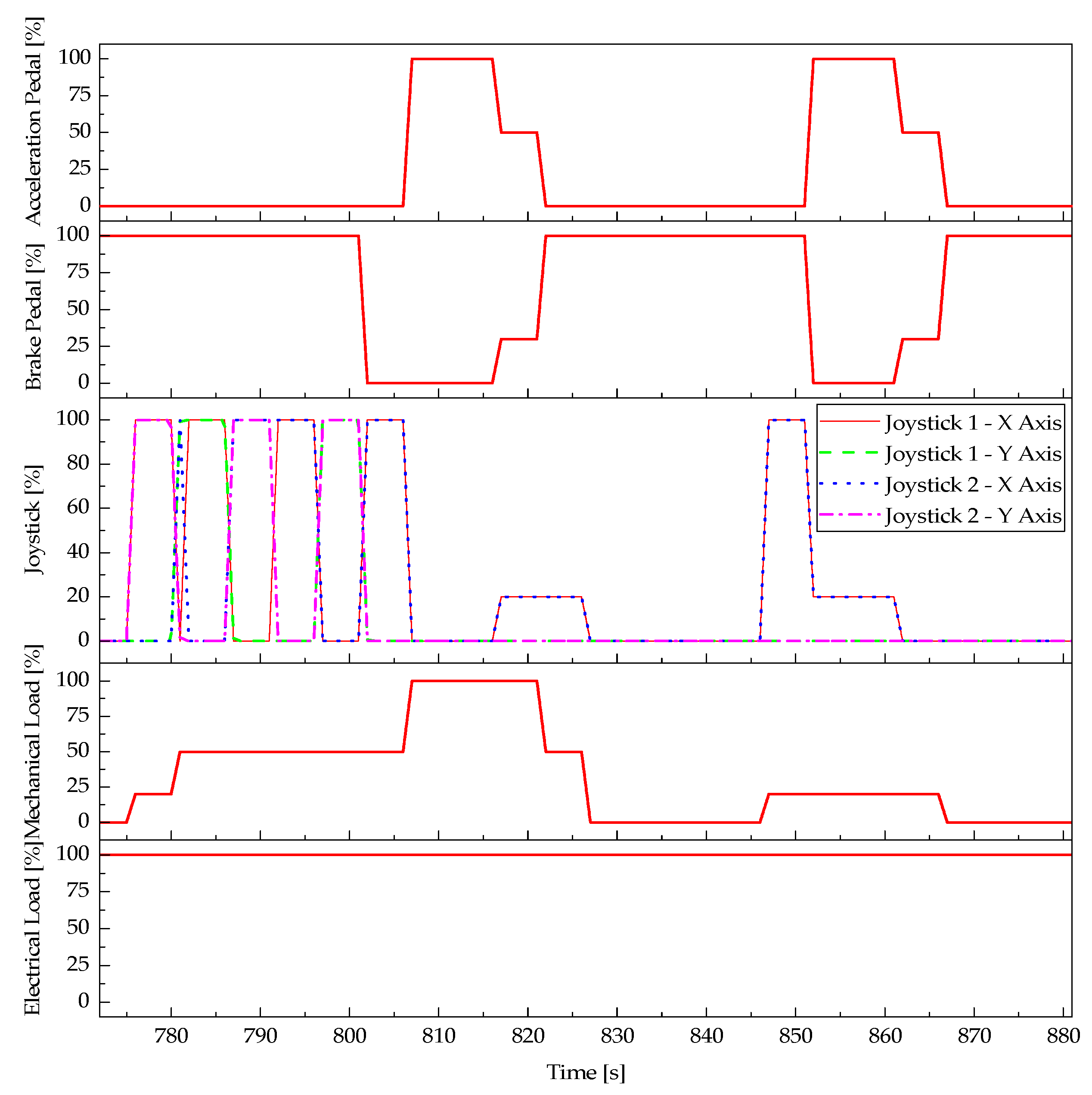
• Both these controllers receive the commands from the joysticks and pedals and then converted them into speed command, ${\overline{n}}_{ICE}$ normalized within range 0 to 1, and brake command, $b{r}_{ICE}$ with on/off logic only, of the ICE as follows (${\overline{n}}_{ICE}=1$ corresponds to the maximum speed command):

  $${\overline{n}}_{ICE}=k_1\sqrt{J{X}_1^2+J{X}_2^2+J{Y}_1^2+J{Y}_2^2}+k_{2}AP\left(100-BP\right),{\overline{n}}_{ICE}=[0,1]$$

  (9)

  $$\{\begin{array}{l}b{r}_{ICE}=0,\mathrm{IF}:{\overline{n}}_{ICE}=0\\ b{r}_{ICE}=1,\mathrm{Otherwise}\end{array}$$

  (10)

  where: k₁ and k₂ are the conversion gains which can be varied through different machine types and by different manufacturers. In this case, the gain are both set to 0.5. These ICE speed and brake commands are then sent to the ECU to regulate the output power of the engine.
• Sampling rate is set to 0.01 s.

5.2.2. Simulation Results

The simulations have been then performed with the two controllers for a test case consisting of 11 cycles defined in Section 5.2.1. First, the influences of the GPM on the ICE mode command and its resulting speed-torque when using the PISSC were investigated through the first 08 cycles as shown in Figure 15. For the easy understanding, the ICE modes, NOR, IDL and STO, are in turn represented by numbers 2, 1 and 0 in the bottom sub-plot of Figure 15 (the STA mode is automatically integrated into NOR or IDL modes). This figure points out that the GPM was activated after the first six working cycles. During the first 06 cycles, the ICE mode commands were resulted from the timer-based mode detection based on its threshold value (3 s) and the RBC (Section 4.4). After these six cycles, based on the HMI value and ICE torque-speed responses, any new machine stages could be directly detected by the GPM. Subsequently, the mode commands could be sent to the ECU 3 s sooner due to the prediction use. This is clearly indicated through the differences of the ICE mode commands’ durations and speed profiles before and after the GPM activation (as bordered by the ‘blue’ and ‘green’ circles in Figure 15).

Next, a comparison of the ICE performances between using the conventional controller and the proposed one were examined. The comparison was performed for one cycle after the GPM was enabled to have the full functionalities of the PISSC. The generated HMI and load signals during this cycle were monitored as in Figure 16. Consequently, the control actions were observed and displayed in Figure 17 while the simulated engine dynamics using the controllers were obtained as plotted in Figure 18.

It is realized that, depending on the HMI commands and mechanical load conditions, the conventional controller without the ISS function always runs the ICE within the normal or idle speed regions. The four cylinders of the engine were activated to produce the output power. Thus, the energy efficiency in the low torque region was low. Especially during the periods without any HMI commands and external load (around 883 s to 846 s and after 873 s), the ICE was operated with ‘zero’ production efficiency and therefore, the fuel was totally wasted. Meanwhile, with the PISSC, the ICE was smoothly driven between the four modes. Once the ‘zero’ work phases started, the ICE was quickly shut down to avoid the efficiency and fuel losses. In addition, during the work tasks, the ICE modes with the cylinder deactivation were controlled based on the exact amount of energy required to enhance the tasks. This can be clarified through the comparisons of the ICE mode decisions (the bottom sub-plot of Figure 17) and the resulting ICE speed profiles (the top sub-plot of Figure 18) using the two control methods with respect to the same working conditions (HMI commands and ICE loads). By utilizing the IDL mode, one cylinder of the ICE could be deactivated during the low load torque condition to save the fuel while still maintained the desired output power. Hence, the fuel economy of the machine could be significantly improved.

In order to evaluate the fuel saving potential of the proposed hybridization technology, the simulated engine performances were carefully analyzed using key performance indicators (KPIs). These KPIs factors mainly consists of the ICE stop/start numbers and durations, amounts of fuel used/saved and their costs.

The analysis was firstly carried out for the first six working cycles as shown in

Table 6. KPI analysis for the simulated ICE performances during the first 06 working cycles.

KPI	KPI’s Unit	CONC	PISSC	Notes
Stop Count	-	1	13	Include initial state of ICE
Start Count	-	0	12	Not include 1st ICE start using key
Run Time	s	668.88	539.87	Total ICE run time
Stop Time	s	0.12	129.13	Total ICE stop time
Fuel Used	L (Litres)	2.06	0.74	Total fuel consumed by ICE
Fuel Saved	L	0	0.14	Against no stop-start function
Total Fuel Saved	L	0	1.32	Against CONC’s total fuel used
% Total Fuel Saved	%	0	64.08	Against CONC’s total fuel used
Fuel Cost Used	£ (Pound 1)	2.39	0.86	Total fuel cost for ICE fuel usage
Fuel Cost Saved	£	0	0.16	Against no stop-start function
Total Fuel Cost Saved	£	0	1.53	Against CONC’s total fuel cost

¹ The fuel price is calculated based upon the average diesel price in UK (£1.16/L—source [21]).

while the GPM was inactive. In case the CONC without ISS function was used, there was a 0.12 s ICE stop time. This was due to the delay in response of the engine when the machine was started the first time by the operator using the machine key. By only looking at the stop-start function of the PISSC, for each cycle, the ICE had to be stopped and then started twice. The ICE run time was reduced from 668.88 s (with the CONC) to 539.87 s (with the PISSC, the ICE was totally shut down for 129.13 s). This, consequently, could lead to a fuel savings of 0.14 L by utilizing the stop-start function (in this case it was the timer-based stop-start control, as described in Section 4). Overall, it can be seen that due to the use of additional modes, IDL (with cylinder deactivation), STO and STA, the ICE could be efficiently driven with only 0.74 L of diesel. Compared to the fuel used by the ICE using the CONC (2.06 L for the same operation), the amount of fuel used could be reduced of 64.08% by applying the PISSC. This is equivalent to a savings of £1.53 of fuel cost by changing the CONC to the proposed method (£0.16 comes from the stop-start function).

Finally, the KPI analysis was performed for the last five cycles while the GPM was activated and the results are displayed in

Table 7. KPI analysis for the simulated ICE performances during the last 05 working cycles.

KPI	KPI’s Unit	CONC	PISSC	Notes
Stop Count	-	0	10
Start Count	-	0	10
Run Time	s	553.02	414.70	Total ICE run time
Stop Time	s	0	138.32	Total ICE stop time
Stop Time due to GPM	s	0	30.71	Estimated stop time due to GPM
% Stop Time due to GPM	%	0	22.20	Against total ICE stop time
Fuel Used	L	1.71	0.53	Total fuel consumed by ICE
Fuel Saved	L	0	0.15	Against no stop-start function
Total Fuel Saved	L	0	1.18	Against CONC’s total fuel used
% Total Fuel Saved	%	0	69.00	Against CONC’s total fuel used
Fuel Cost Used	£ (1)	1.98	0.61	Total fuel cost for ICE fuel usage
Fuel Cost Saved	£	0	0.17	Against no stop-start function
Total Fuel Cost Saved	£	0	1.37	Against CONC’s total fuel cost

¹ The fuel price is calculated based upon the average diesel price in UK (£1.16/L—source [21]).

. Here, two new KPIs, additional stop time due to the GPM activation and its percentage, are used to evaluate the impact of the GPM. As presented in Section 4 and demonstrated through Figure 15, the GPM is capable of reducing the power range or shutting down the engine almost directly when the low or ‘zero’ load are detected, respectively. Based on the average stop time of ICE with the timer-based stop-start function given in Table 6, 21.52 s/cycle (129.13 s over 06 cycles), the additional amount of engine stop time achieved through the last 05 cycles after enabling the GPM can be simply derived as 30.71 s, or an average of 3.07 s stop time was additionally gained through each stop-start action (there were 10 stop-start times counted during these five cycles). Furthermore, as shown in Table 6, the delay in response of the engine was 0.12 s. Therefore, the additional stop time gained by using the GPM was 2.95 s per each stop-start event. This matches exactly the threshold value set for the timer (3 s, for the timer-based stop-start function during the first six cycles). As a result, the total amount of diesel saved during the last five cycles using the PISSC was 1.18 L (or 69%) compared to the traditional control method. The additional fuel saving amount of 4.92% was attained by activating the GPM. This proves evidently the energy saving potential of the proposed PISSC.

6. Conclusions

This paper develops an energy management strategy for construction machines using the novel prediction-based idle-stop-start control approach. The target machine type is firstly selected and the powertrain model is constructed for the PISSC utilization. The PISSC is then designed for a capability of estimating the machine states to directly decide and shift the ICE working regions between its modes in order to maximize the machine efficiency as well as fuel economy.

Through the feasibility study on the targeted excavator and defined test case, the simulation results imply that by using the proposed approach, the ICE could be automatically and proficiently moved into idle or shut down during the low or zero working loads, especially with repeatable working cycles (the GPM was activated after six cycles). Above 66% of the total fuel (average level over 11 cycles of the simulated test case) in case of using the CONC could be reduced by using the PISSC. During the operation with low workloads, the fuel could be saved by utilizing cylinder deactivation technology. Meanwhile in the low idle regions without workloads, most of fuel consumed by the ICE could be saved by employing the stop-start technique.

As stated in a report by the United States Environmental Protection Agency [22], for the U.S. market alone, if the construction industry could reduce fuel consumption by 10%, the reduction in CO₂ would equate to 6.73 million metric tons. From the global market data, it was also indicated that the U.S. market accounts for around 19% of the global market (through the period 2006 to 2018 as reported in [23]). Consequently, a total of 35.42 million metric tons of CO₂ would be eliminated if 10% fuel used by OHCMs around the world could be lessened. Therefore, the proposed approach offers a high potential to achieve this energy saving and emission targets.

To confirm the accuracy of simulation results and to prove confidently the energy saving and emission reduction capability, in Part B of this research, a comprehensive analysis and validation of the proposed methodology is carried out by mean of experiments using a real-time control framework and a Hardware-In-the-Loop test methodology.

References

1. Albers, J.; Meissner, E.; Shirazi, S. Lead-acid batteries in micro-hybrid vehicles. J. Power Source 2011, 196, 3993–4002. [Google Scholar] [CrossRef]
2. Canova, M.; Guezennec, Y.; Yurkovich, S. On the control of engine start/stop dynamics in a hybrid electric vehicle. J. Dyn. Syst. Meas. Control 2009, 131, 061005. [Google Scholar] [CrossRef]
3. Fontaine, C.; Delprat, S.; Guerra, T.M.; Paganelli, S.; Duguey, J.F. Improving micro hybrid vehicles performances with the maximum principle. IFAC Proc. Vol. 2011, 18, 9727–9732. [Google Scholar] [CrossRef]
4. Ozdemir, A.; Mugan, A. Stop-Start System Integration to Diesel Engine and System Modelling and Validation. IFAC Proc. Vol. 2013, 46, 95–100. [Google Scholar] [CrossRef]
5. Rafiei, A.; Ghodsi, M.; Al-Yahmedi, A. Smart stop-start strategy for samand micro-hybrid based on traffic qualification. In Proceedings of the 24th Iranian Conference on Electrical Engineering (ICEE), Shiraz, Iran, 10–12 May 2016; pp. 1187–1192. [Google Scholar]
6. Rizoug, N.; Feld, G.; Bouhali, O.; Mesbahi, T. Micro-hybrid vehicle supplied by a multi-source storage system (battery and supercapacitors): Optimal power management. In Proceedings of the 7th IET International Conference on Power Electronics, Machines and Drives (PEMD), Manchester, UK, 8–10 April 2014; pp. 1–5. [Google Scholar]
7. Schaeck, S.; Stoermer, A.O.; Hockgeiger, E. Micro-hybrid electric vehicle application of valve-regulated lead–acid batteries in absorbent glass mat technology: Testing a partial-state-of-charge operation strategy. J. Power Source 2009, 190, 173–183. [Google Scholar] [CrossRef]
8. Dinh, T.Q.; Marco, J.; Greenwood, D.; Harper, L.; Corrochano, D. Powertrain modelling for engine stop–start dynamics and control of micro/mild hybrid construction machines. IMechE Part K J. Multi-Body Dyn. 2017, in press. [Google Scholar] [CrossRef]
9. Park, K.S.; Kim, S.I.; Jeong, H.J. Low Idle Control System of Construction Equipment and Automatic Control Method Thereof. U.S. Patent US2013/0289834 A1, 31 October 2013. [Google Scholar]
10. Frellch, T.A.; Michael, S. Autoadaptive Engine Idle Speed Control. U.S. Patent US2014/0053801 A1, 27 Februry 2014. [Google Scholar]
11. Holt, G.D.; Edwards, D.J. Analysis of united kingdom off-highway construction machinery market and its consumers using new-sales data. J. Constr. Eng. Manag. 2013, 139, 529–537. [Google Scholar] [CrossRef]
12. Lewis, P.; Leming, M.; Rasdorf, W. Impact of engine idling on fuel use and CO2 emissions of nonroad diesel construction equipment. J. Manag. Eng. 2012, 28, 31–38. [Google Scholar] [CrossRef]
13. Livelink: Latest Technology to Help Manage Your Fleet. Available online: https://gunn-jcb.com/aftermarket/livelink/ (accessed on 7 July 2017).
14. Matsumoto, I.; Nishida, H. Internal Combustion Engine Having Solenoid-Operated Valves and Control Method. U.S. Patent US6332446 B1, 25 December 2001. [Google Scholar]
15. Deng, J.L. Control problem of grey system. Syst. Control Lett. 1982, 1, 288–294. [Google Scholar]
16. Dinh, T.Q.; Ahn, K.K.; Nguyen, T.T. Design of an advanced time delay measurement and a smart adaptive unequal interval grey predictor for real-time nonlinear control systems. IEEE Trans. Ind. Electron. 2013, 60, 4574–4589. [Google Scholar]
17. Geng, N.; Zhang, Y.; Sun, Y.; Jiang, Y.; Chen, D. Forecasting China’s annual biofuel production using an improved grey model. Energies 2015, 8, 12080–12099. [Google Scholar] [CrossRef]
18. Dinh, T.Q.; Ahn, K.K. An accurate signal estimator using a novel smart adaptive grey model SAGM(1,1). Expert Syst. Appl. 2012, 39, 7611–7620. [Google Scholar]
19. Kim, D.; Goh, T.; Park, M.; Kim, S. Fuzzy sliding mode observer with grey prediction for the estimation of the state-of-charge of a lithium-ion battery. Energies 2015, 8, 12409–12428. [Google Scholar] [CrossRef]
20. Zeng, F.; Cheng, X.; Guo, J.; Tao, L.; Chen, Z. Hybridising human judgment, AHP, grey theory, and fuzzy expert systems for candidate well selection in fractured reservoirs. Energies 2017, 10, 447. [Google Scholar] [CrossRef]
21. Regional Fuel Prices. Available online: http://www.fleetnews.co.uk/costs/fuel-prices/ (accessed on 7 July 2017).
22. Truitt, P. Potential for Reducing Greenhouse Gas Emissions in the Construction Sector; USA Environmental Protection Agency: Washington, DC, USA, 2009.
23. Phillips, D. The Changing Structure of the Global Construction Equipment Industry; Off-Highway Research: Frankfurt, Germany, 2013; Available online: http://bub.vdma.org/documents/105686/790347/2013-01%20Philips.pdf/92096e4f-98f1-4560-8412-4f2d72fd8cfd (accessed on 1 April 2017).
Figure 1. Representative configuration of the target machine powertrain.
Energies 10 00962 g001
Figure 2. Components’ model set built in AMESim.
Energies 10 00962 g002
Figure 3. Complete Simulink plan model using AMESim and Simscape.
Energies 10 00962 g003
Figure 4. Engine control architecture integrated PISSC approach for a construction machine.
Energies 10 00962 g004
Figure 5. PISSC-based engine working principle. *; ** and *** denote signals entering ‘Cycle Data Rolling Operation’ block. The internal structure of this block is described in Figure 6.
Energies 10 00962 g005
Figure 6. Flow diagram of the cycle data rolling operation and GPM modules.
Energies 10 00962 g006
Figure 7. ICE working regions to define ICE modes.
Energies 10 00962 g007
Figure 8. Logics for NOR mode decision.
Energies 10 00962 g008
Figure 9. Logics for IDL mode decision.
Energies 10 00962 g009
Figure 10. Logics for STO mode decision.
Energies 10 00962 g010
Figure 11. Logics for STA mode decision.
Energies 10 00962 g011
Figure 12. Validation results of three powertrain models with respect to the first cranking experiment.
Energies 10 00962 g012
Figure 13. Validation results of three powertrain models with respect to the second cranking experiment.
Energies 10 00962 g013
Figure 14. Complete Simulink control system for simulations.
Energies 10 00962 g014
Figure 15. Simulated ICE mode command and speed response using PISSC during the first eight cycles.
Energies 10 00962 g015
Figure 16. Simulated HMI and load signals from the 7th cycle—stage 16 to the 8th cycle—stage 15.
Energies 10 00962 g016
Figure 17. Simulated ICE control inputs from the 7th cycle —stage 16 to the 8th cycle—stage 15.
Energies 10 00962 g017
Figure 18. Simulated ICE dynamics from the 7th cycle —stage 16 to the 8th cycle—stage 15.
Energies 10 00962 g018