Article

Diagnosis and Early Warning of Wind Turbine Faults Based on Cluster Analysis Theory and Modified ANFIS

1
State Key Laboratory of Power Transmission Equipment & System Security and New Technology, School of Electrical Engineering, Chongqing University, Chongqing 400044, China
2
State Grid Lishui Electric Power Supply Company, Lishui 323000, China
3
State Grid Chengdu Power Supply Company, Chengdu 610041, China
*
Author to whom correspondence should be addressed.
Energies 2017, 10(7), 898; https://doi.org/10.3390/en10070898
Submission received: 30 March 2017 / Revised: 12 June 2017 / Accepted: 22 June 2017 / Published: 1 July 2017

Abstract

:
The construction of large-scale wind farms results in a dramatic increase of wind turbine (WT) faults. The failure mode is also becoming increasingly complex. This study proposes a new model for early warning and diagnosis of WT faults to solve the problem of Supervisory Control And Data Acquisition (SCADA) systems, given that the traditional threshold method cannot provide timely warning. First, the characteristic quantity of fault early warning and diagnosis analyzed by clustering analysis can obtain in advance abnormal data in the normal threshold range by considering the effects of wind speed. Based on domain knowledge, Adaptive Neuro-fuzzy Inference System (ANFIS) is then modified to establish the fault early warning and diagnosis model. This approach improves the accuracy of the model under the condition of absent and sparse training data. Case analysis shows that the effect of the early warning and diagnosis model in this study is better than that of the traditional threshold method.

1. Introduction

The generation of energy by using wind power has been applied widely in recent years because of its non-polluting and renewable nature. Most wind power plants are sparsely distributed in grasslands, deserts (e.g., Gobi desert), coastal seas, and other harsh natural environments. Given this condition, wind turbine (WT) failure occurs frequently and imposes high maintenance costs. Improving the reliability of WT operations and reducing the cost of wind power has attracted research attention [1,2,3,4]. The failure of most of the equipment in WTs is a gradual process. This finding means that the fault of WTs is usually experienced from its occurrence to the development, from mild to severe. The running data of some status parameters, which indicate that faults will range from normal to fault state, can possibly detect these abnormal characteristics in potential faults or during the early fault detection period. Thus, the reliability of WTs has been modified by preventing the occurrence or development of faults.
At present, the diagnosis and early warning of WT faults has attracted considerable attention among researchers. SJ Watson analyzed output power by wavelet analysis and discovered fault monitoring [5]. Lu B analyzed the influence of pitch system stability when it is affected by air load in actual operations and further reduced the fan load to reduce the corresponding downtime of WTs [6]. Radoslaw Zimroz divided the state of WTs into normal, mild, and severe states by fitting the characteristic value and power when operating at variable operating conditions of stochastic wind speed. The purpose of early warning was achieved by analyzing the deviation degree between the running data and the three states [7]. Z Hameed monitored the state parameters of the sudden failure of WTs with a condition monitoring system and guaranteed its running state using a fault detection system [8]. These studies achieved good results, but the generation mechanism of WT faults and the complexity of the running state of WTs’ influence mechanism require further investigation. Achieving highly accurate diagnosis and early warning of WT faults despite lack of relevant historical data is also worthy of in-depth investigation.
This study proposes a new WT fault early warning and diagnosis model. Status monitoring parameters from the Supervisory Control And Data Acquisition (SCADA) system are analyzed by k-means clustering analysis method. An early warning model is then established to realize early warning and fault diagnosis based on the modified Adaptive Neuro-fuzzy Inference System (ANFIS) algorithm [9,10,11]. Finally, the effectiveness and accuracy of the model is verified by a case study of unit #7 in a wind farm in North China.

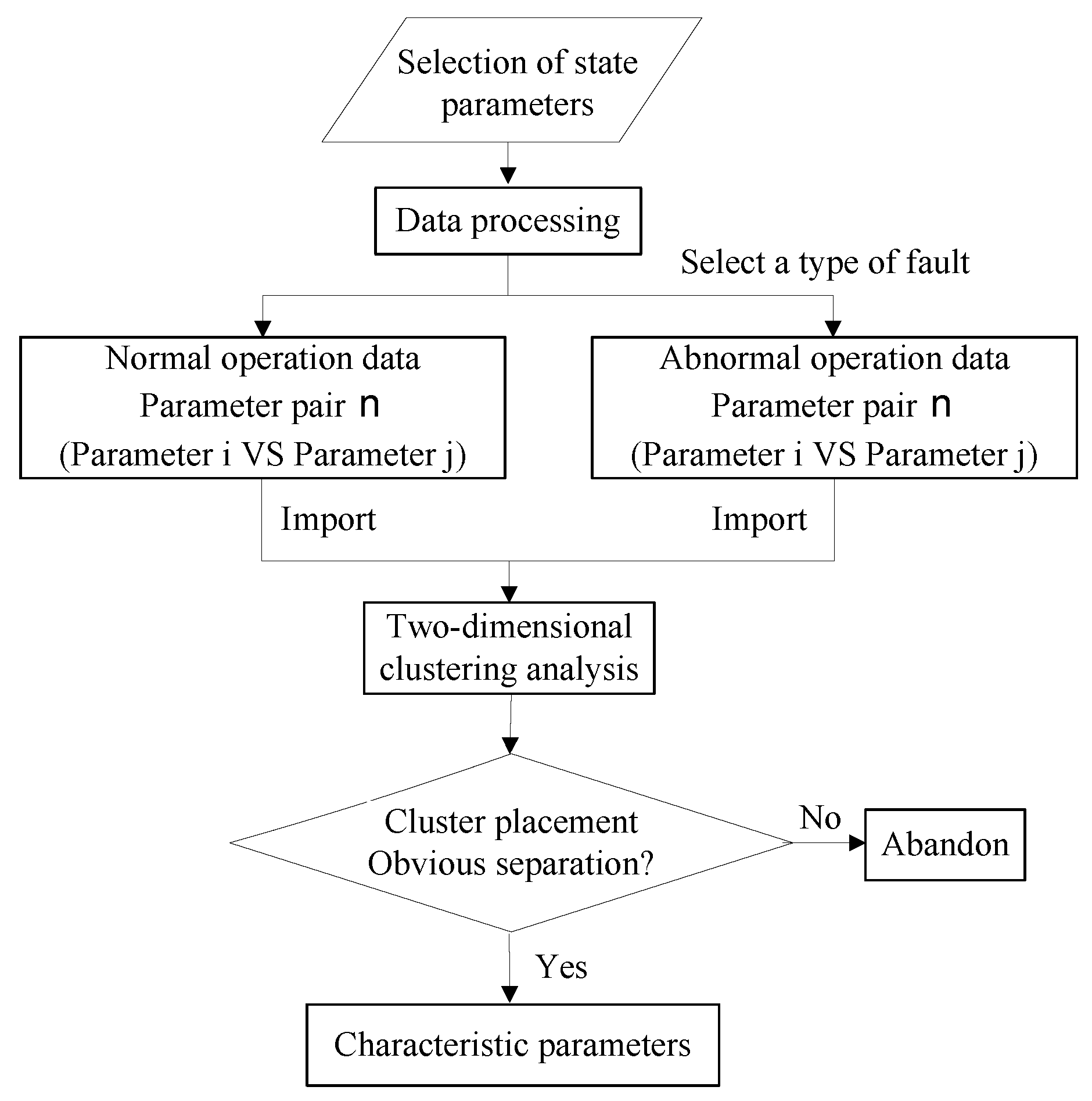
2. Analysis of Characteristic Parameters

K-means clustering algorithm was first proposed by J.B. MacQueen in 1987 [12]. First, it calculates the Euclidean distance between the data objects and cluster centers. Then, it differentiates clusters according to the dissimilarity measures of clusters, which take the minimum square sum of the Euclidean distance error as a criterion function. Finally, it performs optimal classification of the initial clustering center vector (V = V1, V2, ..., Vk) and achieves the minimum value of evaluation index E by continuous optimization of criterion function. Its specific process can be described as follows.
Step 1
Taking data set { x 1 , x 2 , . . . , x n } as input samples, where x n R n .
Step 2
k data points are selected randomly from the data object as the initial clustering center, and it can be expressed as μ 1 , μ 2 , , μ k R n .
Step 3
Calculating the Euclidean distance between each observation point and each clustering center di,j, and d i , j = | | x i μ j | | .
Step 4
According to the principle of minimum Euclidean distance, each observation point is classified into the corresponding clustering object.
Step 5
Calculating the average value of each clustering object, and the average value is taken as the new clustering center.
Step 6
Repeating Step 3, Step 4 and Step 5 until two consecutive E values change is no more than 10%, or the number of iterations reaches 100 times.
E = i = 1 k x C i | | x i c i | | 2
where E represents square sum of the Euclidean distance, xi represents the data object of cluster Ci, and ci is the center of cluster Ci.
When the WT fails, each fault will result in different state parameters that depart from the normal data bandwidth in different degrees. On the other hand, the cluster of the fault parameters will be evidently separated when analyzing the state parameters of the fault by k-means clustering; the clustering center will also be significantly different [13]. The analysis of WT fault characteristic parameters based on cluster analysis is shown in Figure 1.
In Figure 1, two different parameters make up a parameter pair and act as the horizontal and vertical coordinates of the 2D clustering graph. The cluster placement of each kind of fault data is generally different from that of the normal data. The key to using these two parameters as the representative of the characteristic parameter pair can be described as follows: the clustering of fault data and that of normal data are clearly separated, and the clustering center evidently deviates. Otherwise, it cannot be used as the characteristic parameter of this type of fault.

3. Modified ANFIS of the WT Fault Early Warning Model

ANFIS is an effective method for constructing the complex nonlinear relationship between input and output. ANFIS is more accurate and efficient than other methods as it integrates the advantages of neural networks and fuzzy systems. However, the accuracy and effectiveness of the ANFIS algorithm will be substantially reduced when training data are sparse. This study combines favorable rules into the ANFIS training program according to domain knowledge and proposes a fuzzy Takagi-Sugeno-Kang (TSK) model based on rule center [14,15,16,17].

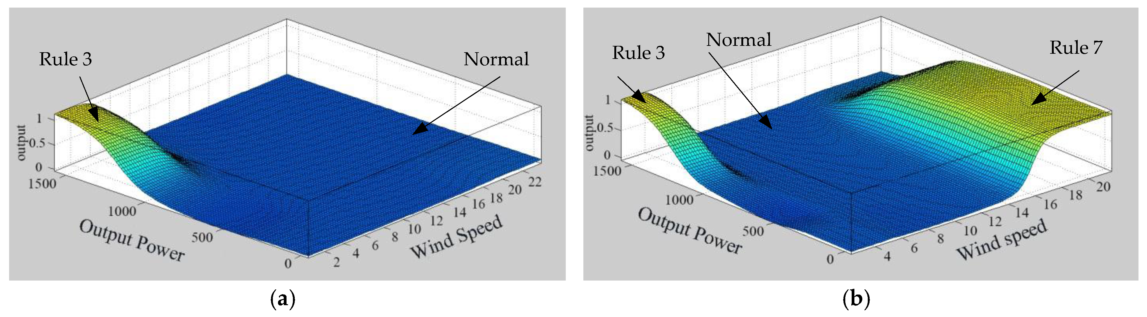
3.1. Domain Knowledge Rules

The favorable rule for fault diagnosis of WTs indicates that the rule and running state of the wind unit are mismatched at the maximum degree. This finding means that fault can be easily detected. By taking the fault detection of the power curve of WTs as an example, three membership-grade functions, namely, “low”, “medium”, and “high”, are used to express the state parameters of output power and wind speed. Thus, the rule 3 × 3 = 9 can be obtained, as shown in Figure 2.
In Figure 2, two different parameters comprise a parameter pair and act as the horizontal and vertical coordinates of the 2D clustering graph. The cluster placement of each kind of fault data is generally different from that of the normal data. The key to using these two parameters as the representative of the characteristic parameter pair can be described as follows: the clustering of fault data and that of normal data are clearly separated, and the clustering center evidently deviates. Otherwise, it cannot be used as the characteristic parameter of this type of fault.

3.2. Modified ANFIS Model

3.2.1. Principle Analysis

A typical ANFIS model is composed of five layers, and the fourth layer is the defuzzification layer; thus, each of the rules will obtain a clear output in this layer [18,19,20]. All nodes in this layer are adaptive, and its output is the product of the normalized emission intensity and the first-order polynomial function:
O i 4 = w ¯ i f i = w ¯ i ( p i x + q i y + r i ) . i = 1 , 2
In Formula (2), w ¯ i is the outputs of the third layer of the ANFIS structure, { p i , q i , r i } are the posterior parameter set. The Taylor series is expanded in Formula (2) as:
f i f i ( c i ) + d f i d x 1 i ( x 1 i c 1 i ) + + d f i d x n i ( x n i c n i )
where n represents the dimension of the input, f i ( c i ) is the basic function value of the ith rule center, and d f i / d x n i is the function gradient of the ith rule center. c i = [ c 1 i , . . . , c n i ] represents the rule center, which has the same dimension with the input. Thus, the first-order model of ANFIS can be expressed as:
f i = 1 R ( f i ( c i ) + n = 1 N ( x n i c n i ) ) w ¯ i
In this formula, f i ( c i ) can be obtained through zero-order ANFIS model. Domain knowledge is merged into the model in the form of Gauss basis function, as follows:
Φ r j = a j exp ( i = 1 n ( c i B c i F σ i j ) 2 )
where jJ, rR, and JR form part of Set J, which is the favorable rule of Set R. B and F are two different data sets, c i B = ( c 1 B , c 2 B , . . . c i B . . . c n B ) and c i F = ( c 1 F , c 2 F , . . . c i F . . . c n F ) are the centers of rth and jth rules presents in sets B and F respectively. The Gauss basis function is used to simulate the domain knowledge. When several favorable rules exist, the output of the model in the rth rule can be expressed as the weighted geometric mean of the independent Gauss function:
m 0 r = j = 1 J ( Φ r j ) γ r j
γ r j = 1 i = 1 J ( D r j / D r i )
where m 0 r is the parameter produced by the rth rule of the zero-order ANFIS model. γ r j represents the weight of the degree between the rth rule centers and jth favorable rule centers.

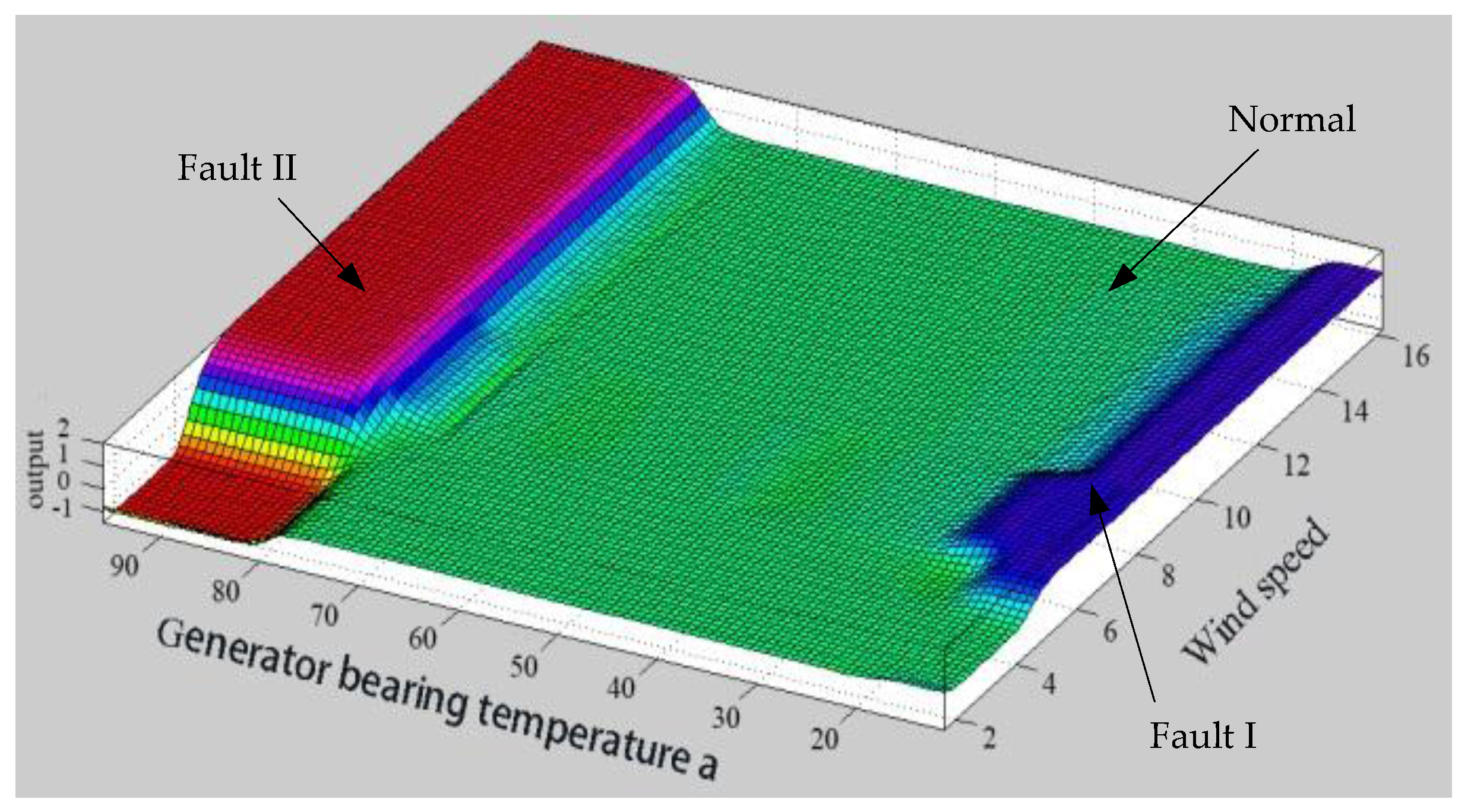
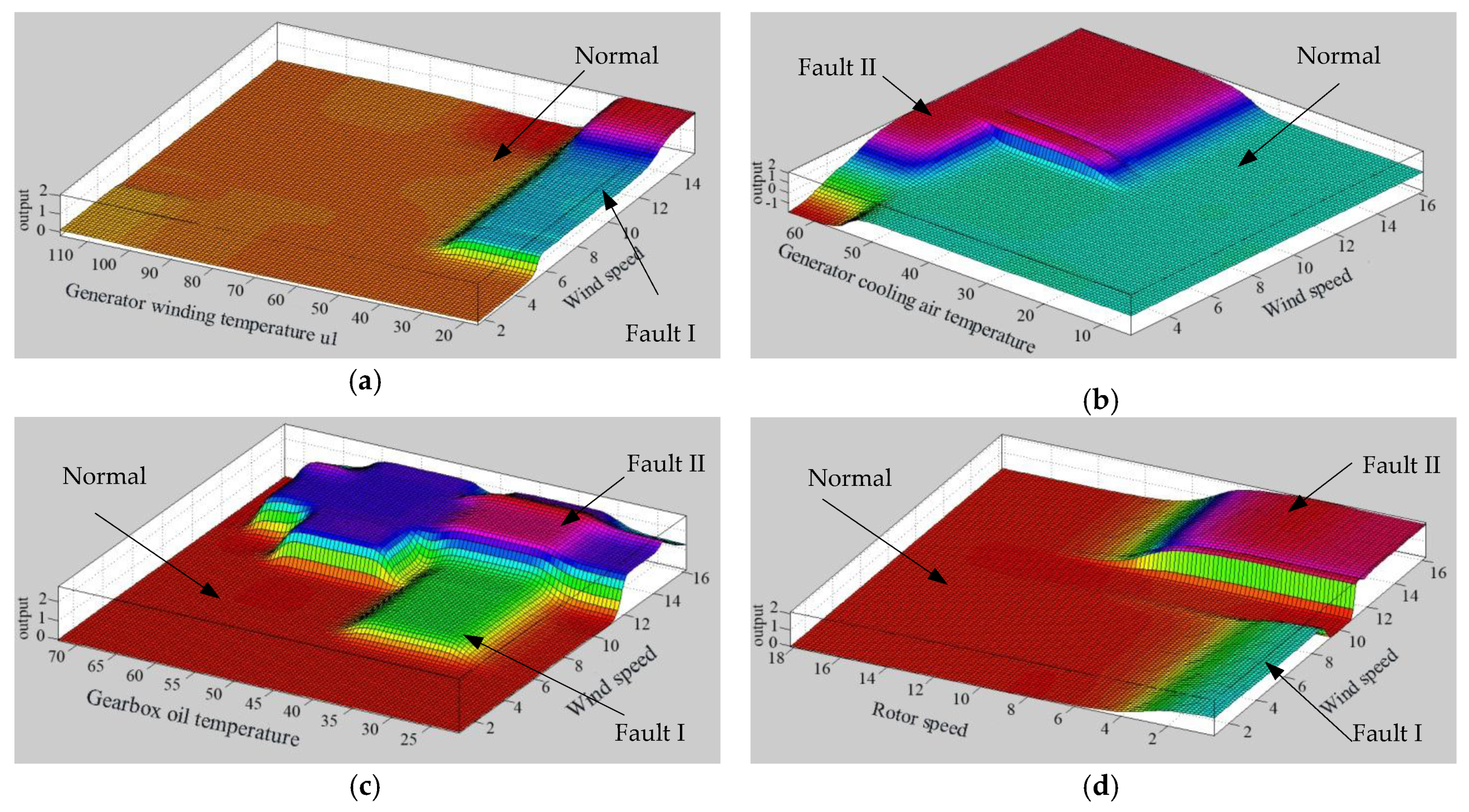
3.2.2. Model Verification

The traditional ANFIS model and the modified ANFIS model are used to identify the fault of the output power curves (input 1 is the wind speed, input 2 is the output power, output = 1 represents fault, and output = 0 represents the normal state). A total of 1000 normal data and 50 abnormal data are used for training the two models. Each input contains three membership-grade functions, the maximum step size is 150. The minimum error is approximately 0.01. The results are shown in Figure 3.
Figure 3a shows that the performance of the traditional ANFIS model is different from Figure 2 in the rule 7 region because of the lack of data in the corresponding rule 7. This result is inconsistent with actual detection. However, the modified ANFIS model obtained good results because it incorporated the domain knowledge into the training model. As shown in Figure 3b, the results of the modified ANFIS model is consistent with Figure 2 in the rule 7 region even in the absence of training data in the corresponding rule 7. The results show that the modified ANFIS algorithm performs well when the input data is noisy or when the input data is sparse.

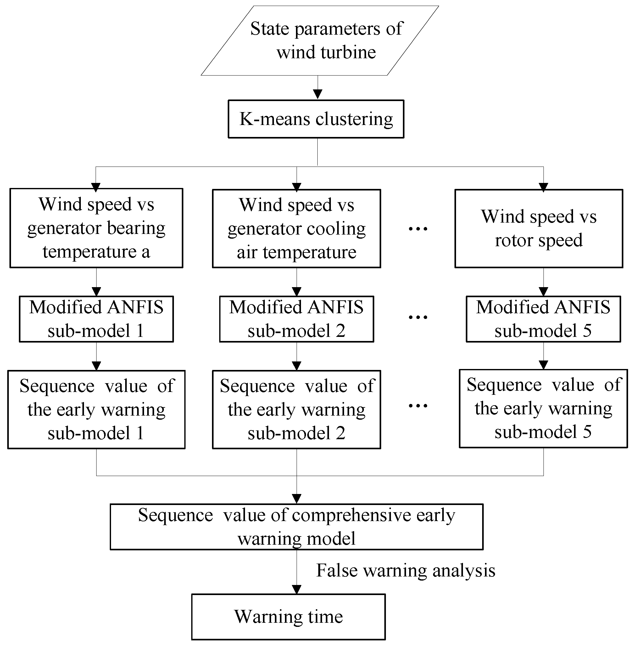
3.3. Comprehensive Early Warning Model and Its Effect Analysis

3.3.1. Comprehensive Early Warning Model

The running state of a WT is significantly influenced by wind speed. Thus, the time series of wind speed is selected as the operating condition and reference sequence. This study takes generator bearing temperature a, generator winding temperature u1, generator cooling air temperature, gearbox oil temperature, and rotor speed as state parameters of WTs [21,22,23]. The time series of these parameters act as a comparative sequence. Given that these parameters are not consistently affected by wind speed, this study uses grey correlation algorithm to calculate the correlation degree between the parameters and wind speed. The higher the degree of correlation, the more consistent the influence of wind speed is, which indicates the increasingly evident influence of wind speed. Moreover, the change trend with wind speed will be separated from the original consistency when fault occurs [24,25,26]. Notably, the corresponding fault data evidently deviate from the normal data in the 2D clustering graph. The warning effect will then improve. The comprehensive early warning model can be expressed as:
O U T P U T = i = 1 5 o u t p u t i × r i i = 1 5 r i
where OUTPUT is the warning output value of the comprehensive early warning model, and o u t p u t i is the warning output value for each characteristic quantity warning sub model. Symbol i indicates the set of early warning sub models, which is higher than the warning threshold in the early warning output value figure. The “5” indicates the number of features to test, which are: generator bearing temperature a, generator winding temperature u1, generator cooling air temperature, gearbox oil temperature, and rotor speed, respectively.

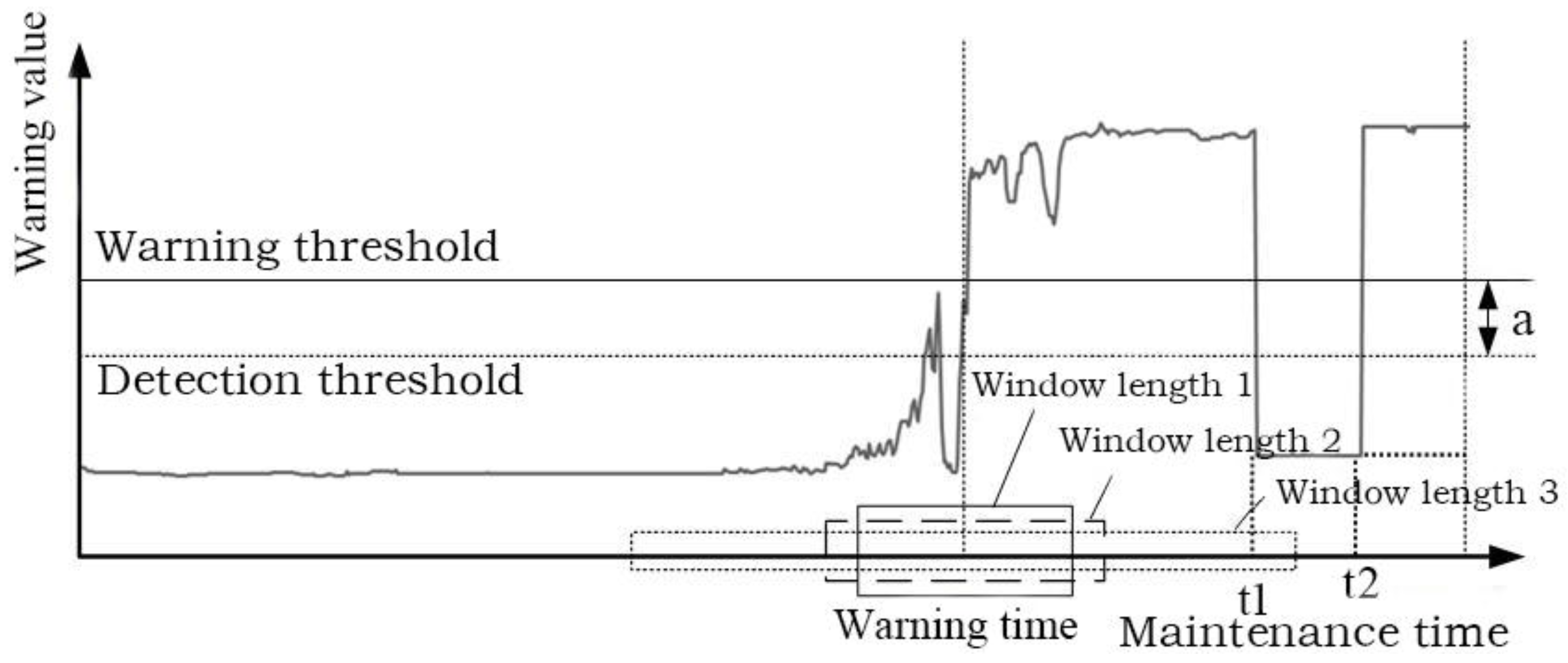
3.3.2. False Warning Analysis

Although the modified ANFIS early warning model can identify the fault and normal states to a certain extent, the value of the warning threshold will affect the accuracy of early warning to some degree. The output value will also fluctuate when parameters change, similar to the wind speed in Figure 3, which will cause a false alarm. As shown in Figure 4, after the early warning output value exceeded the threshold for a certain period, it returns to the normal range at t1 and maintains the normal state along the dotted line in Figure 4, which shows the false alarm. In addition, the warning value returned to the normal range after it exceeded the warning threshold for a period at t1 in Figure 4. However, the warning value exceeded the warning threshold again at t2 and kept running over the warning threshold, which means that the alarm is normal.
To reduce the probability of a false alarm, this study introduces the concepts of “window length”, “detection threshold”, “early warning effective value”, and “early warning possible value”. The definitions are as follows.
Window length is a period selected on the time axis with the warning time as the center, with Window Lengths 1, 2, and 3, as shown in Figure 4.
Detection threshold represents data that are constantly lower than the warning threshold, as shown in Figure 4.
Early warning effective value can be interpreted as follows.
Assuming that the number of points in window length is M, which has exceeded the warning threshold, the total number of points in window length is N, then the m/N is called the early warning effective value.
As shown in Figure 4, the effective value of the alarm m/N is calculated with Window Lengths 1, 2, and 3. Different window lengths then lead to different calculated effective values of the alarm. For example, window lengths 1 and 2 are too short to be fully considered as the warning values after the warning time, window length 3 is taken as the warning value after warning time for consideration, and the warning value returns to the normal range after t1. Thus, m and m/N are lower. The analysis shows that the window length significantly influences the effectiveness of the alarm.
A warning effective value m/N substantially less than 60% indicates a false alarm. This situation occurs only when the warning values return to normal after the warning time, which shows that the pseudo fault has been ruled out, and the fan is in normal operation. Therefore, a false alarm occurs when m/N is considerably less than 60%.
This study set a detection threshold to fully consider the change of the early warning value before the early warning time. The situation can be fully taken into account if any point fluctuates in the “detection threshold” and “warning threshold”, or if any point gradually changes from “detection threshold” to “warning threshold” in the early warning time as the detection threshold is lower than the warning threshold.
This study suggests that the number of points greater than the detection threshold before the time of half the warning window length is m1. Thus, the expression of m1/(N/2) is considered a possible value of warning. The bigger the possible warning value is, the greater the possibility that the alarm is normal. However, the value may also be 0 when the warning value exceeds the warning threshold mutation. Thus, the value can be used as an auxiliary criterion of alarm probability.

3.3.3. Selection of False Alarm Parameter

This study sets the best early warning threshold, window length, and validity of early warning based on the data analysis of the confusion matrix [27]. The confusion matrix analysis presents the actual maintenance information and early warning information obtained by the early warning system, as defined in Table 1.
In Table 1, True Positive (TP) is defined as the correct prediction of the actual maintenance events with maintenance, False Positive (FP) is the wrong prediction of the actual maintenance events with no maintenance, False Negative (FN) represents the wrong prediction of the actual maintenance events with maintenance, and True Negative (TN) is defined as the correct prediction of the actual maintenance events with no maintenance.
Further data analysis is shown as follows according to the above definition.
A C C = T P + T N T P + F P + T N + F N
Accuracy (ACC) is the proportion of correctly predicted events in the total forecast events. It is one of the key factors to determine whether a program is effective or not.
E R = F P + F N T P + F P + T N + F N
Error Rate (ER) is the proportion of events mistakenly predicted in the total forecast events. ER is usually expressed as ER = 1 − ACC.
R C = T P T P + F N
Recall (RC) is the correct proportion of forecasts with actual repair. The greater the amount of this representation is, the better the effect is, because the failure to be found can lead to a catastrophic failure.
P = T P T P + F P
Precision (P) is the proportion of actual maintenance in the case of predictive maintenance. A high value is preferred because it can avoid the additional costs caused by virtual maintenance.
Therefore, the TP, FN, FP, and TN can be determined along with the actual maintenance information and early warning information of the wind field. According to Formulas (9)–(12), the value table of ACC, ER, RC, and P can be obtained in different early warning thresholds, window lengths, and effective values of early warning. Therefore, the optimal warning threshold, optimal window length, and optimal effective warning value can be selected according to the table. Substitute the selected parameters into the early warning model to obtain the alarm moment under the best alarm threshold.

4. Case Analysis

Emergency shutdown is taken as an example, which occurred in a wind field in North China in 16 March 2015 at 9:31. The alarm bell rang at 9:31 with “error generator fan pump heater protection” warning. To prevent this accident, the fault diagnosis model is established to verify the validity of the diagnostic effect based on cluster analysis theory and the modified ANFIS [28].
For the two types of malfunctions involved, K-means clustering analysis is adopted to establish the 2D clustering analysis of the relationship between the five characteristic quantities and wind speed. Then, on the basis of the clustering analysis, the improved ANFIS algorithm is employed to establish the malfunction warning sub-model. The two methods shall verify each other; clustering analysis acts as an effective way to screen malfunction characteristic quantity and as the prerequisite for the entire research. Next, the five warning sub-models are used to establish the comprehensive warning model, and the false alarms of the model are further explored on the basis of the Confusion matrix. Finally, the output value of the warning is derived for this case of malfunction.

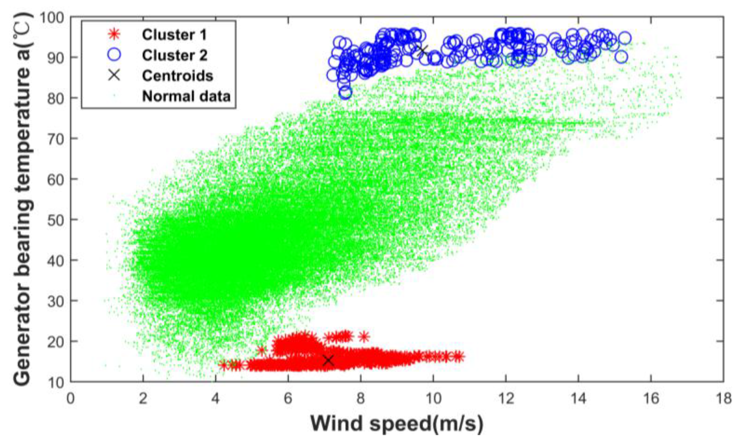
4.1. Analysis of Fault Feature Parameters

To avoid the clustering error caused by the cluster number k, the SCADA data of all units in a wind farm in North China from January 2014 to July 2015 were analyzed. Along with maintenance records, two types of the most frequent failure modes were selected, namely, Fault I called “generator low temperature operation fault” and Fault II called “generator shaft temperature overheat fault”. To ensure that the number of data objects in the two clusters is nearly the same and to avoid errors due to the serious asymmetry of data objects to further generate clustering effect deviation, the numbers of Faults I and II are 272 and 327 groups, respectively. Cluster analysis was performed with the example of “‘speed vs. generator bearing temperature a”, and normal data were introduced into the generated cluster analysis chart. The results are shown in Figure 5.
As shown in Figure 6, k-mean clustering algorithm divides the two kinds of data objects into two clusters, and the two clusters are completely separated, as shown in Figure 6, with “red *’”and “blue O”. The data objects in the two clusters are closely linked. That is, the clustering results can meet the requirements of high diversity in the cluster and high similarity among clusters. The results show that the k-mean clustering analysis method has a good clustering effect on the fault set. Figure 6 shows that the normal data are separated from the fault data, and the clustering placements of the two kinds of faults deviate from the bandwidth of the normal data placement. Therefore, WT has Fault I when the data fall in the region of “red *” and has Fault II when the data fall in the region of “blue O”. The state parameters of the “speed vs. generator bearing temperature a” can be used as a characteristic parameter pair for the fault classification and early warning.
The other four characteristic quantities are obtained in the same way, as shown in Figure 7. In Figure 7, the normal data have few clustering fault map fusions. For example, the fault data of Fault II fall in the bandwidth of the normal data in Figure 7a. However, the fault data of Fault I can be clearly identified. Therefore, the characteristic quantity enhances the identification of Fault I. Similarly, the characteristic quantity in Figure 7b enhances the identification of Fault II. The data of two kinds of faults exhibit evident separation with the above method in Figure 5 and Figure 6. At least one kind of fault data is far from the placement bandwidth of normal data. Thus, all characteristic quantities can be used to classify the corresponding faults.

4.2. Warning Sub-Model

An early warning sub-model for WTs is established based on the modified ANFIS model. The warning sub-model of the five characteristic parameter pairs is shown, as follows:
P i = [ I i , 1 , I i , 2 , O i ] T i [ 1 , 2 , 3 , 4 , 5 ]
where Ii,1 and Ii,2 are the inputs of the five parameters, and Oi is the corresponding output. The values of Oi are 0, 1, and 2, because only two kinds of faults exist. These faults represent the normal state, Fault I, and Fault II, respectively.
Taking the characteristic parameter pair of “wind speed vs. generator bearing temperature a as an example (input 1 is the wind speed, and input 2 is the generator bearing temperature a) and setting the training step as 2000 and the minimum error as 0.01, then the early warning sub-model is obtained, as shown in Figure 8.
In Figure 8, the output value of Fault I is mainly 1, Fault II is mainly 2, and the normal case is mainly 0. Therefore, the state of the WT can be divided into normal state, Fault I, and Fault II through the threshold setting. That is, the model can realize the function of fault early warning and diagnosis. The other four early warning sub-models are obtained in the same way, as shown in Figure 9.

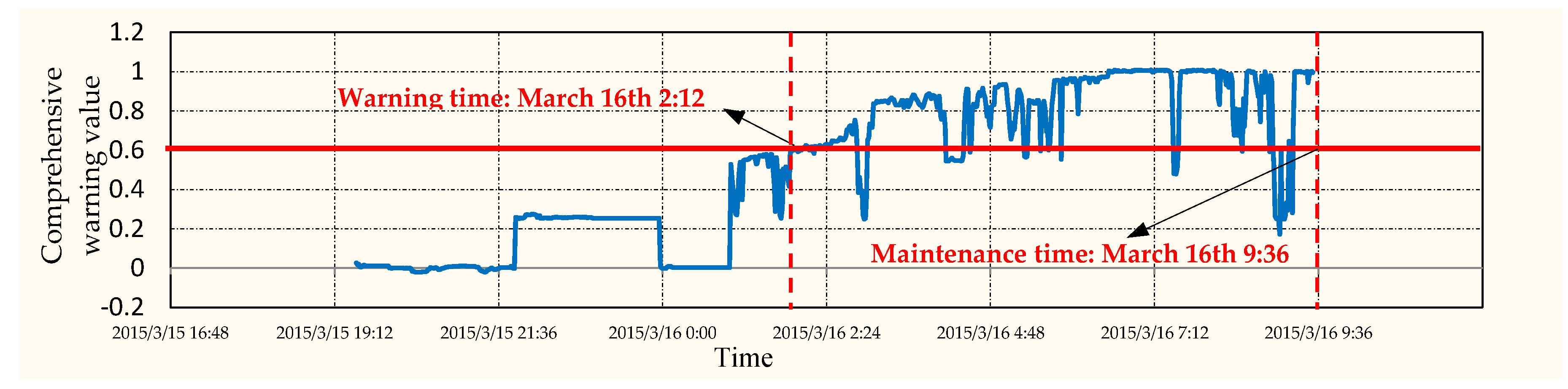
4.3. Comprehensive Analysis of the Early Warning Result

There were 40 groups of failure data and 40 groups of normal data selected from Fault I. These data were integrated into the actual maintenance and early warning information. The table of ACC, ER, RC, and P in different early warning thresholds, window lengths, and warning RMSs are then obtained, as shown in Table 2.
As shown in Table 2, ACC achieves a maximum of 97.5%, which ensures the highest warning accuracy when the warning threshold value is 0.6, the window length is 40 min, and the early warning valid value is 25%. Although the RC value is only 95%, it is enough to ensure that all of the faults are found as much as possible and to avoid potentially catastrophic failure. P achieves a maximum of 100%. Thus, the extra cost of virtual maintenance can be completely avoided. Therefore, the warning threshold value of 0.6 is the optimal setting. In the same way, the warning threshold value of 1.5, the window length of 40 min. Warning valid value greater than 25% is the best setting for Fault II.
The operation data of WT from 19:31 of 15 March 2015 to 9:31 of 16 March 2015 are imported into the comprehensive warning model in sequence. The warning threshold is set as follows: if the output value is less than 0.6, it is considered normal; if the output value is greater than 0.6 but less than 1.5, it belongs to Fault I; if the output value is greater than 1.5, it belongs to Fault II. Finally, the comprehensive chart under the optimal threshold is shown in Figure 10.
Figure 10 shows that the warning output value exceeded 0.6 at 2:12 on 16 March 2015. Fluctuations then ranged from 0.6 to 1. In other words, this fault is Fault I, which is called “generator low temperature operation fault”. The early warning threshold value reached 0.6 for the first time at 1:52 on 16 March 2015 and the window length was 40 min. The number of the points where the value is more than the warning threshold is 20 (M = 20) during the window length, and the total number of points of N is 40. Therefore, the early warning valid value is 50% > 25%, which is an effective early warning. Thus, the real warning time can be calculated as (warning time + window length)/2, that is, 2:12 on 16 March 2015. This time is 7 h and 19 min earlier than the threshold warning time of the SCADA system on 9:31 on 16 March 015. The effect is superior to that of the traditional threshold method.

5. Conclusions

This study presented a new model of WT fault early warning and diagnosis based on the data mining analysis of SCADA data in a wind power plant. The main conclusions are as follows.
(1)
The fault parameter pair of a WT was analyzed by k-means cluster analysis. Furthermore, the abnormal data in the normal threshold range can be found in advance.
(2)
An early warning and diagnosis model was established based on the fault characteristics. The accuracy of the model in the absence of training data, sparse conditions were enhanced by improving the ANFIS algorithm with domain knowledge.
(3)
The concepts of “window length”, “detection threshold”, “effective value of early warning”, and “possible value of early warning” were presented in this study to determine at the false alarm of early warning model. These concepts comply with actual failure data and maintenance data of wind farms.
(4)
In the example, the actual fault was recognized within 7 h and 19 min ahead of the threshold warning time of the SCADA system with this model. The function of fault diagnosis and early warning was achieved, and the effect was better than that of the traditional threshold method.

Acknowledgments

This work was supported by the Funds for Innovative Research Groups of China (51321063) and The National Natural Science Fundation of China (5150070514).

Author Contributions

Study concepts were proposed by Quan Zhou and Taotao Xiong. Simulation analysis, data processing, and the manuscript preparation were done by Taotao Xiong and Mubin Wang. Data analysis and interpretation were done by Quan Zhou, Taotao Xiong, Chenmeng Xiang, Qingpeng Xu. Manuscript editing was performed by Taotao Xiong and Mubin Wang.

Conflicts of Interest

The authors declare no conflict of interest.

References

  1. Kusiak, A.; Li, W. Virtual Models for Prediction of Wind Turbine Parameters. IEEE Trans. Energy Convers. 2010, 25, 245–252. [Google Scholar] [CrossRef]
  2. Jiang, C.; Liu, W.; Zhang, J.; Liu, D. Risk assessment of generation and transmission systems considering wind power penetration. Trans. Chin. Electrotech. Soc. 2014, 29, 260–270. [Google Scholar]
  3. Abdelrahem, M.; Kennel, R. Fault-Ride through Strategy for Permanent-Magnet Synchronous Generators in Variable-Speed Wind Turbines. Energies 2016, 9, 1066. [Google Scholar] [CrossRef]
  4. Qiu, Y. Study of Wind Turbine Fault Diagnosis Based on Unscented Kalman Filter and SCADA Data. Energies 2016, 9, 847. [Google Scholar]
  5. Wason, S.J.; Xiang, B.J.; Yang, W.; Tavner, P.J.; Crabtree, C.J. Condition monitoring of power output of wind turbine generators using wavelets. IEEE Trans. Energy Convers. 2010, 25, 715–721. [Google Scholar] [CrossRef]
  6. Lu, B.; Li, Y.; Wu, X. A review of recent advances in wind turbine condition monitoring and fault diagnosis. In Proceedings of the IEEE Conference on Power Electronics and Machines in Wind Applications (PEMWA09), Lincoln, NE, USA, 24–26 June 2009; pp. 1–7. [Google Scholar]
  7. Radoslaw, Z.; Walter, B.; Tomasz, B. Diagnostics of bearings in presence of strong operating conditions non-shtionarity-A procedure of load-dependent features processing with application to wind turbine bearings. Mech. Syst. Signal Process. 2014, 46, 16–27. [Google Scholar]
  8. Hameed, Z.; Hong, Y.S.; Cho, Y.M.; Ahn, S.H.; Song, C.K. Condition monitoring and fault detection of wind turbines and related algorithms: A review. Renew. Sustain. Energy Rev. 2009, 13, 1–39. [Google Scholar] [CrossRef]
  9. Jang, J. ANFIS: Adaptive-network-based fuzzy inference systems. IEEE Trans. Syst. Man Cybern. 1993, 23, 665–685. [Google Scholar] [CrossRef]
  10. Buragohain, M.; Mahanta, C. A novel approach for ANFIS modelling based on full factorial design. Appl. Soft Comput. 2008, 8, 609–625. [Google Scholar] [CrossRef]
  11. Zhang, Y.; Zhou, Q.; Sun, C.; Lei, S.; Liu, Y.; Song, Y. RBF Neural Network and ANFIS-Based Short-Term Load Forecasting Approach in Real-Time Price Environment. IEEE Trans. Power Syst. 2008, 23, 853–858. [Google Scholar] [CrossRef]
  12. Kanungo, T.; Mount, D.M.; Netanyahu, N.S.; Christine, D.P.; Ruth, S.; Angela, Y.W. An Efficient k-Means Clustering Algorithm: Analysis and Implementation. IEEE Trans. Pattern Anal. Mach. Intell. 2002, 24, 881–892. [Google Scholar] [CrossRef]
  13. Zhang, X.; Su, B. Vibrant fault diagnosis for hydro-turbine generating unit using minmax kernel K-means clustering algorithm. Power Syst. Prot. Control 2015, 43, 27–34. [Google Scholar]
  14. Johanyák, Z.; Papp, O. A Hybrid Algorithm for Parameter Tuning in Fuzzy Model Identification. Acta Polytech. Hung. 2012, 9, 2012. [Google Scholar]
  15. Precup, R.; David, R.; Petriu, E.; Preitl, S.; Radac, M. Novel Adaptive Charged System Search algorithm for optimal tuning of fuzzy controllers. Expert Syst. Appl. 2014, 41, 1168–1175. [Google Scholar] [CrossRef]
  16. Kıran, M.; Fındık, O. A directed artificial bee colony algorithm. Appl. Soft Comput. J. 2015, 26, 454–462. [Google Scholar] [CrossRef]
  17. Solos, I.P.; Tassopoulos, I.X.; Beligiannis, G.N. Optimizing shift scheduling for tank trucks using an effective stochastic variable neighbourhood approach. Int. J. Artif. Intell. 2016, 14, 1–26. [Google Scholar]
  18. Zhou, Q.; Sun, W.; Zhang, Y.; Ren, H.J.; Sun, C.X.; Deng, J.Y. A new method to obtain load density based on improved ANFIS. Power Syst. Prot. Control 2011, 39, 29–34. [Google Scholar]
  19. Dragomir, O.; Dragomir, F.; Stefan, V.; Minca, E. Adaptive Neuro-Fuzzy Inference Systems as a Strategy for Predicting and Controling the Energy Produced from Renewable Sources. Energies 2015, 8, 13047–13061. [Google Scholar] [CrossRef]
  20. Ahmed, A.; Jun, S.; Senior, M.; Yan, J. Modeling and Simulation of an Adaptive Neuro-Fuzzy Inference System (ANFIS) for Mobile Learning. IEEE Trans. Learn. Technol. 2012, 5, 226–237. [Google Scholar]
  21. Chen, B.; Matthews, P.; Tavner, P. Automated on-line fault prognosis for wind turbine pitch systems using supervisory control and data acquisition. IET Renew. Power Gener. 2015, 9, 503–513. [Google Scholar] [CrossRef]
  22. Lapira, E.; Brisset, D.; Davari Ardakani, H.; Lee, J. Wind turbine performance assessment using multi-regime modeling approach. Renew. Energy 2012, 45, 86–95. [Google Scholar] [CrossRef]
  23. Zaher, A.; McArthur, S. Online wind turbine fault detection through automated SCADA data analysis. Wind Energy 2009, 12, 74–93. [Google Scholar] [CrossRef]
  24. Zheng, X.; Li, M.; Wang, J.; Ren, H.; Fu, Y. Operational conditions classification of offshore wind turbines based on kernel principal analysis optimized by PSO. Power Syst. Prot. Control 2016, 44, 28–35. [Google Scholar]
  25. Li, Y.; Fang, R. Reliability assessment for wind turbine based on weighted degree of improved grey incidence. Power Syst. Prot. Control 2015, 43, 63–69. [Google Scholar]
  26. Yin, Z.; Han, B.; Xie, S. An improved grey correlation algorithm and its application for diesel fault prediction. In Proceedings of the Sixth International Conference on Intelligent Control and Information Processing (ICICIP), Wuhan, China, 26–28 November 2015; pp. 412–416. [Google Scholar]
  27. Kong, Y.; Jing, M. Research of the Classification Method Based on Confusion Matrixes and Ensemble Learning. Comput. Eng. Sci. 2012, 34, 111–117. [Google Scholar]
  28. College of Electrical Engineering, Chongqing University, Shazhengjie, Shapingba, Chongqing, China. Available online: http://www.cee.cqu.edu.cn/Teacherweb_Article.asp?id=1211&tid=1253&y_id=1054 (accessed on 23 May 2017).
Figure 1. Feature extraction flow chart.
Energies 10 00898 g001
Figure 2. Domain knowledge rules.
Energies 10 00898 g002
Figure 3. Training results of the models: (a) traditional Adaptive Neuro-fuzzy Inference System (ANFIS) model; and (b) modified ANFIS model.
Energies 10 00898 g003
Figure 4. False alarm analysis chart.
Energies 10 00898 g004
Figure 5. Case implementation flow chart.
Energies 10 00898 g005
Figure 6. Characteristic quantity “wind speed vs. generator bearing temperature a”.
Energies 10 00898 g006
Figure 7. Characteristic quantities: (a) wind speed vs. generator winding temperature u1; (b) wind speed vs. generator cooling air temperature; (c) wind speed vs. gearbox oil temperature; (d) wind speed vs. rotor speed.
Energies 10 00898 g007
Figure 8. Early warning sub model: Wind speed vs. Generator bearing temperature a.
Energies 10 00898 g008
Figure 9. Early warning sub model: (a) wind speed vs. generator winding temperature u1; (b) wind speed vs. generator cooling air temperature; (c) wind speed vs. gearbox oil temperature; and (d) wind speed vs. rotor speed.
Energies 10 00898 g009
Figure 10. Warning figure in best warning threshold.
Energies 10 00898 g010
Table 1. Confusion matrix analysis table.
Maintenance informationForecast
Maintenance RequiredNo Maintenance Required
RealityMaintenanceTPFN
No maintenanceFPTN
Table 2. Results of confusion matrix analysis.
Window Lengthm/NACC (%)ER (%)RC (%)P (%)
Warning threshold 0
20 min>25%55%45%100%52.63%
40 min>25%57.5%42.5%100%54.05%
20 min>35%60%40%100%55.56%
40 min>35%62.5%37.5%100%57.14%
Warning threshold 0.1
20 min>25%91.25%8.75%97.5%86.67%
40 min>25%75%25%100%66.67%
20 min>35%77.5%22.5%100%68.97%
40 min>35%77.5%22.5%100%68.97%
Warning threshold 0.2
20 min>25%87.5%12.5%100%80%
40 min>25%87.5%12.5%100%80%
20 min>35%88.75%11.75%97.5%82.98%
40 min>35%91.25%8.75%97.5%86.67%
Warning threshold 0.3
20 min>25%90%10%100%83.33%
40 min>25%91.25%8.75%97.5%86.67%
20 min>35%93.75%6.25%95%92.68%
40 min>35%95%5%95%95%
Warning threshold 0.4
20 min>25%93.75%6.25%97.5%92.68%
40 min>25%92.5%7.5%95%90.48%
20 min>35%95%5%95%95%
40 min>35%95%5%92.5%97.37%
Warning threshold 0.5
20 min>25%91.25%6.25%97.5%90.7%
40 min>25%95%5%95%95%
20 min>35%96.25%3.75%92.5%100%
40 min>35%96.25%3.75%92.5%100%
Warning threshold 0.6
20 min>25%93.75%6.25%95%92.68%
40 min>25%97.5%2.5%95%100%
20 min>35%96.25%3.75%92.5%100%
40 min>35%96.25%3.75%92.5%100%
Warning threshold 0.7
20 min>25%92.5%7.5%92.5%92.5%
40 min>25%95%5%90%100%
20 min>35%95%5%90%100%
40 min>35%93.75%6.25%87.5%100%
Warning threshold 0.8
20 min>25%90%10%85%94.44%
40 min>25%91.25%8.75%85%97.14%
20 min>35%90%10%80%100%
40 min>35%87.5%12.5%83.33%100%
Warning threshold 0.9
20 min>25%83.75%16.25%70%96.55%
40 min>25%81.25%18.75%65%96.3%
20 min>35%80%18.75%65%100%
40 min>35%80%18.75%65%100%
Warning threshold 1.0
20 min>25%57.5%42.5%13.33%100%
40 min>25%55%45%9.09%100%
20 min>35%52.5%47.5%4.76%100%
40 min>35%52.5%47.5%4.76%100%

