
Day-Ahead Natural Gas Demand Forecasting Using Optimized ABC-Based Neural Network with Sliding Window Technique: The Case Study of Regional Basis in Turkey


Abstract
:1. Introduction
1.1. Related Work
1.2. Motivation
1.3. Our Contribution
2. Experimental Background
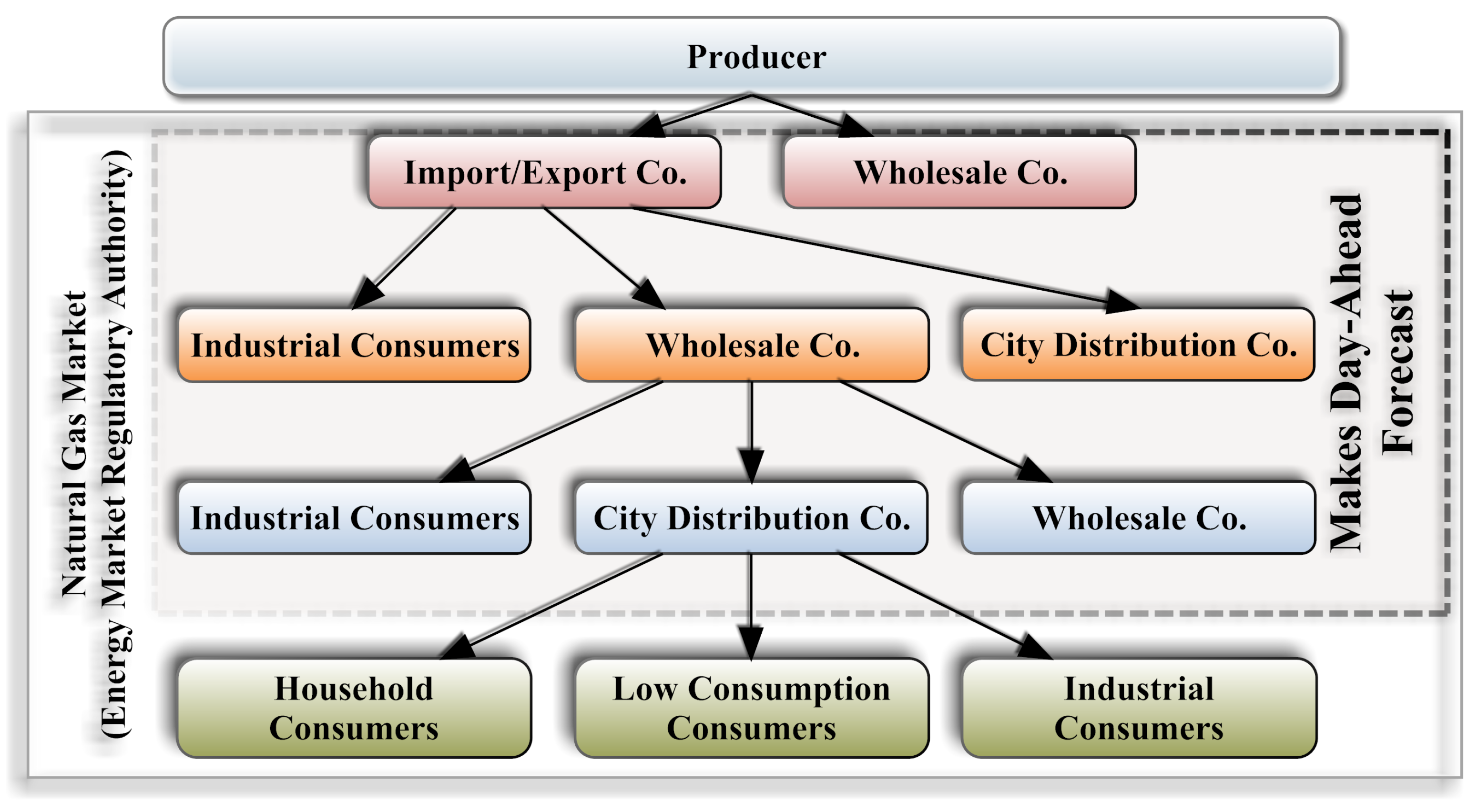
2.1. Natural Gas Consumption in Turkey
2.2. The Preparation of the Data
3. Method
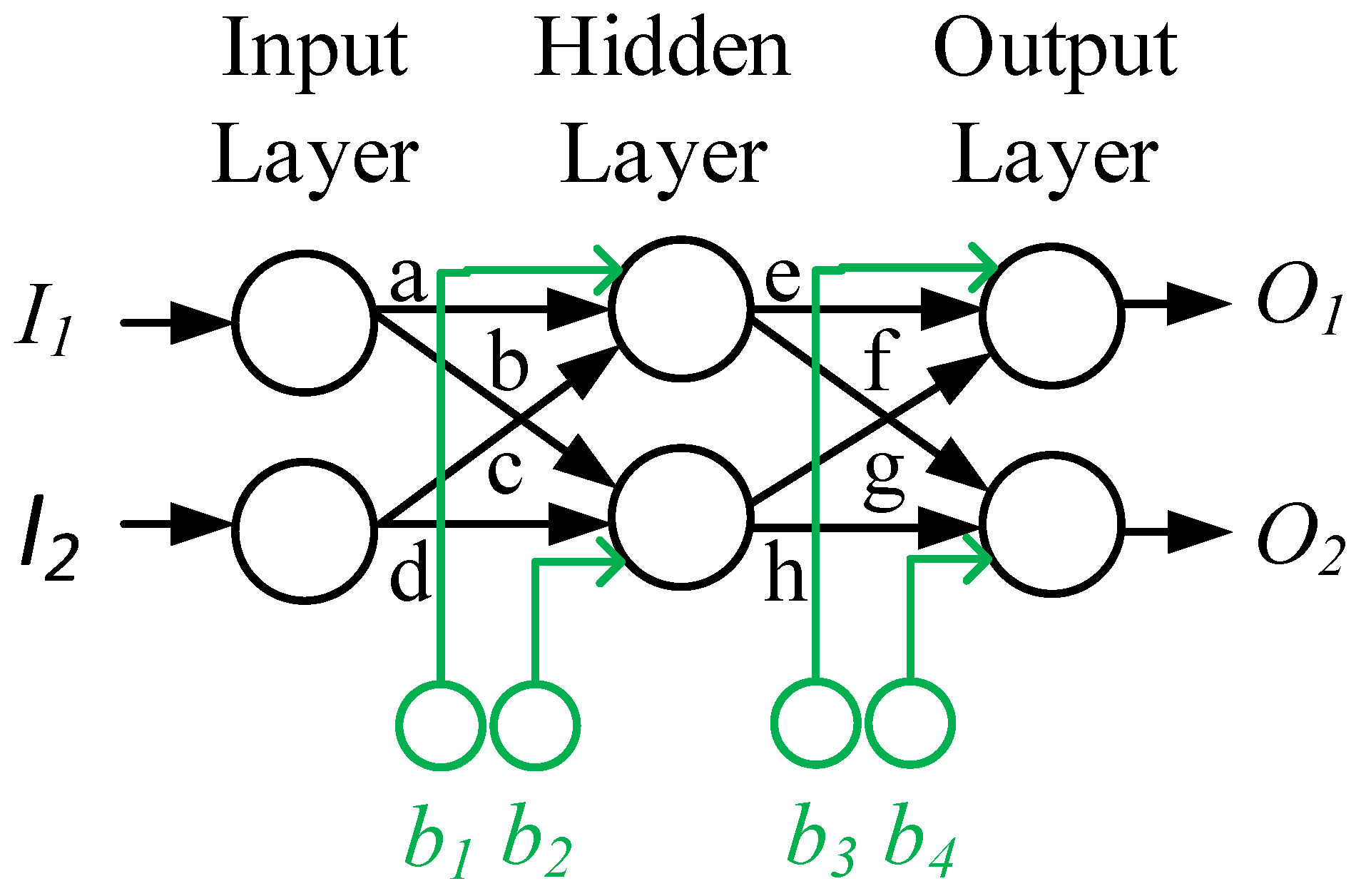
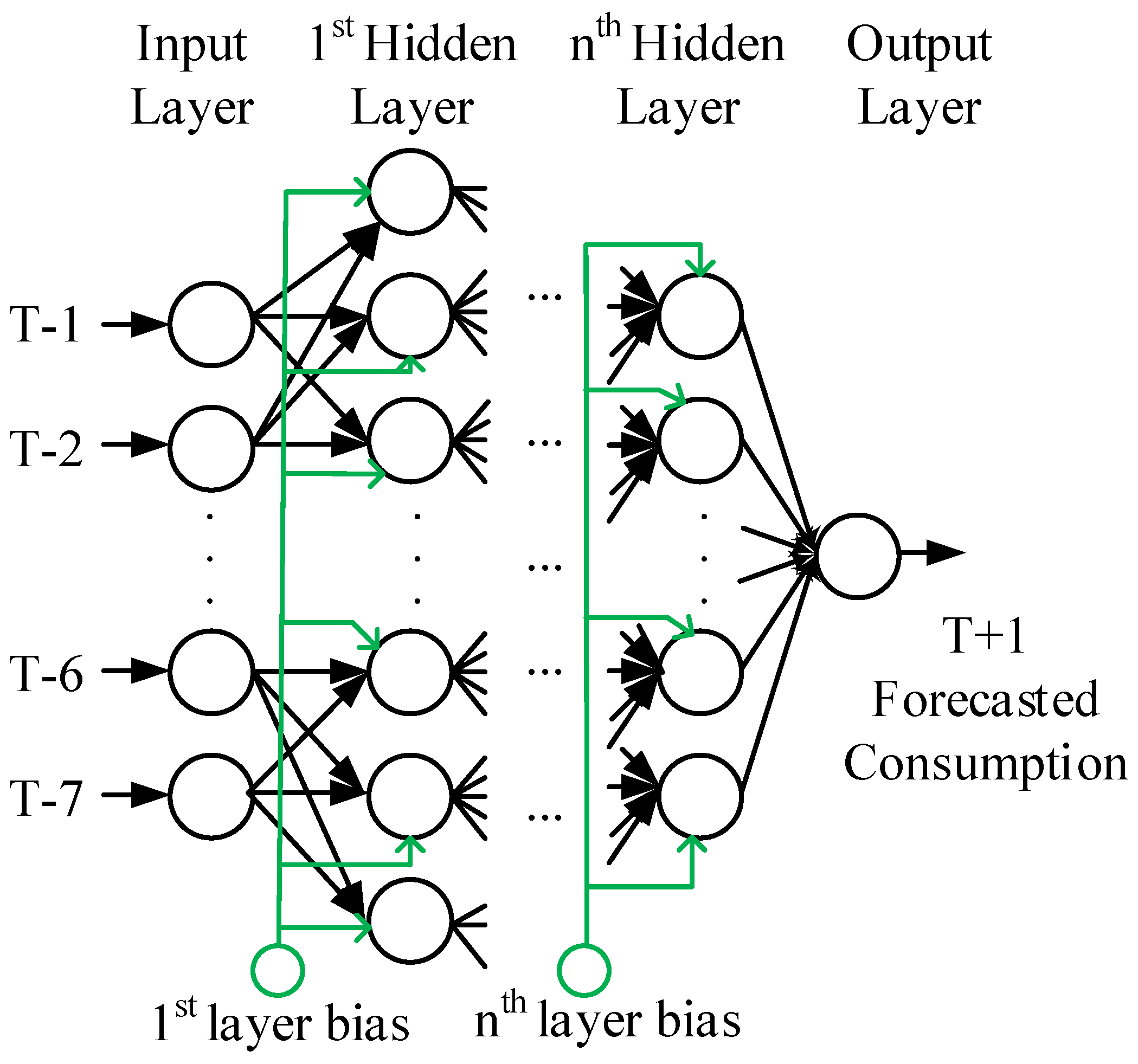
3.1. Artificial Neural Network (ANN)
3.1.1. Feedforward Algorithm
3.1.2. Backpropagation Algorithm
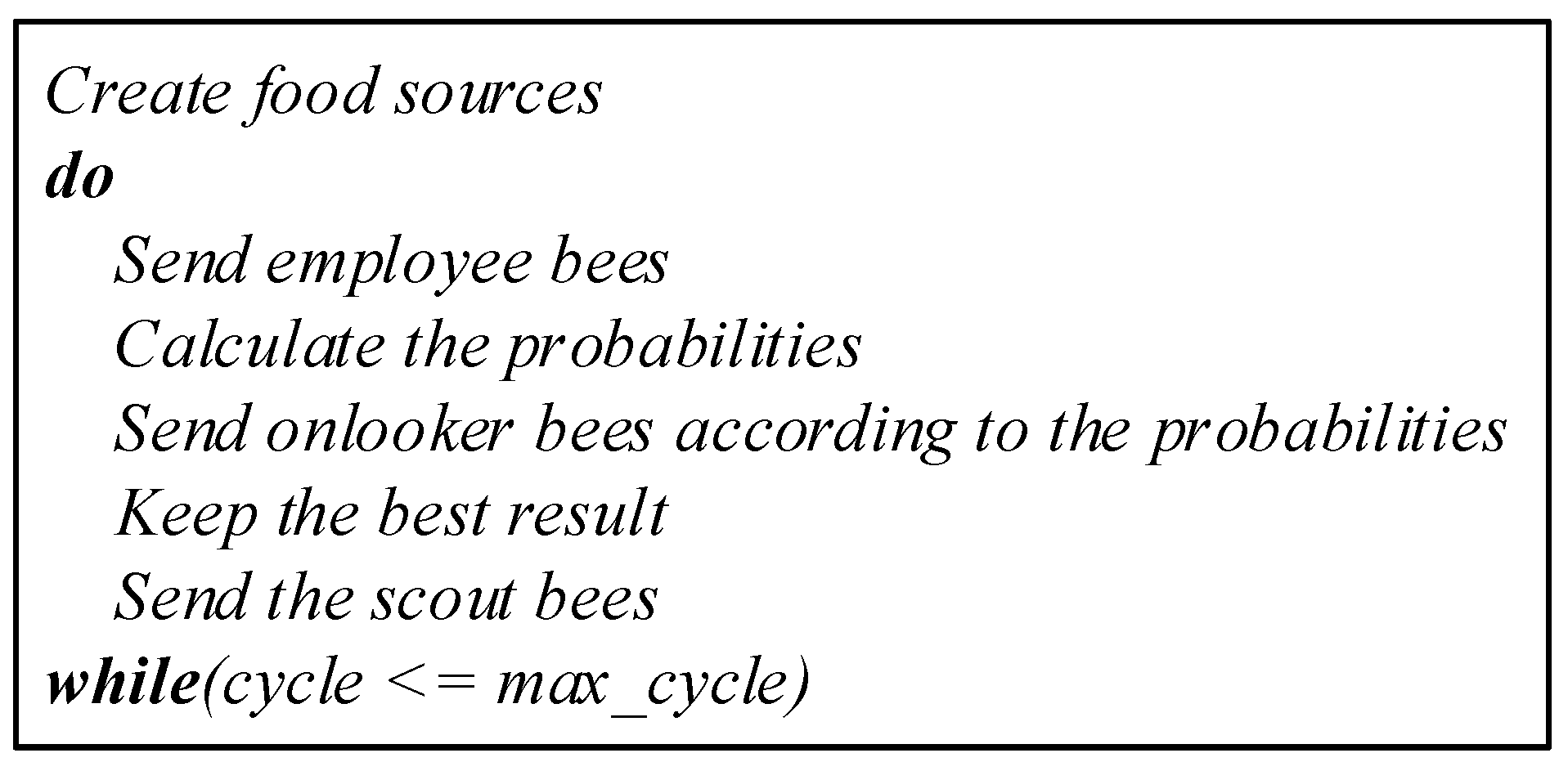
3.2. Artificial Bee Colony Algorithm (ABC)
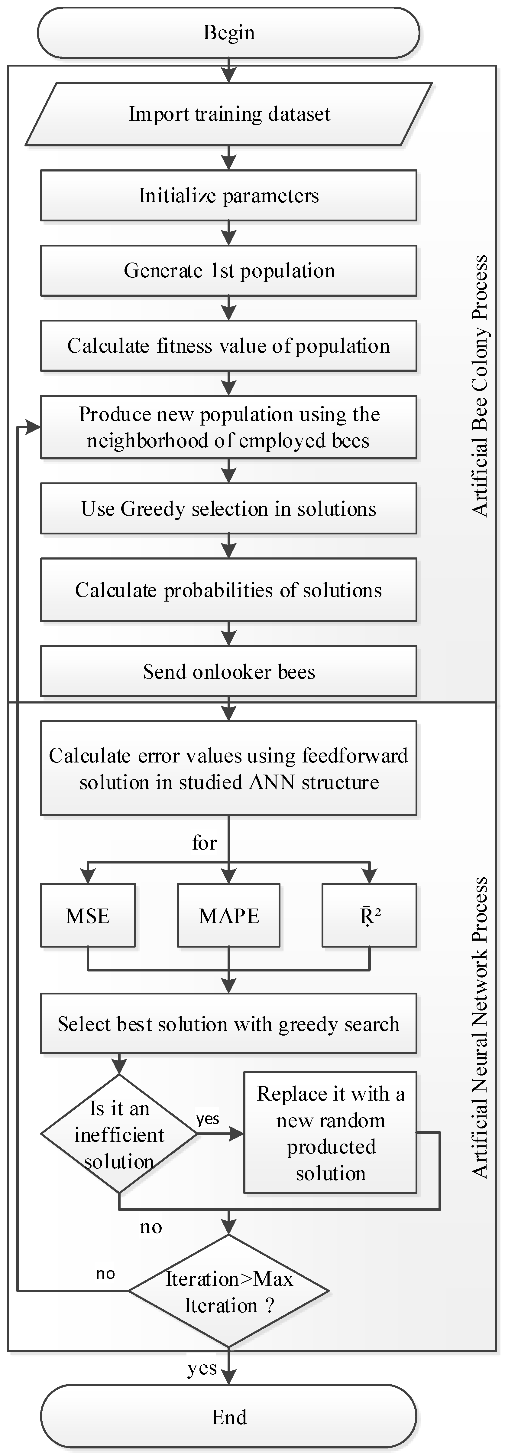
3.3. ABC Based ANN (ANN-ABC)
3.4. Different Training Error Parameters
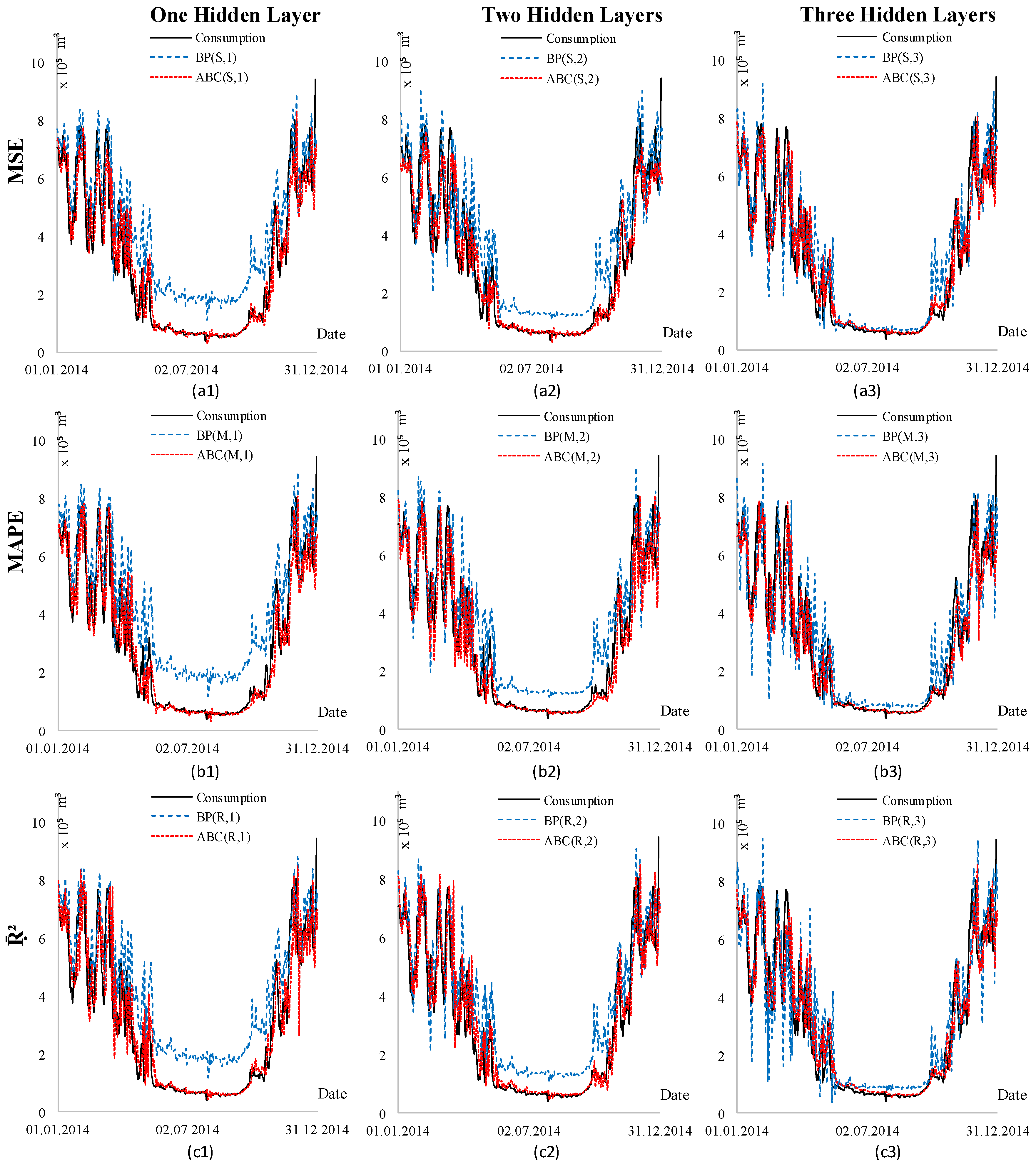
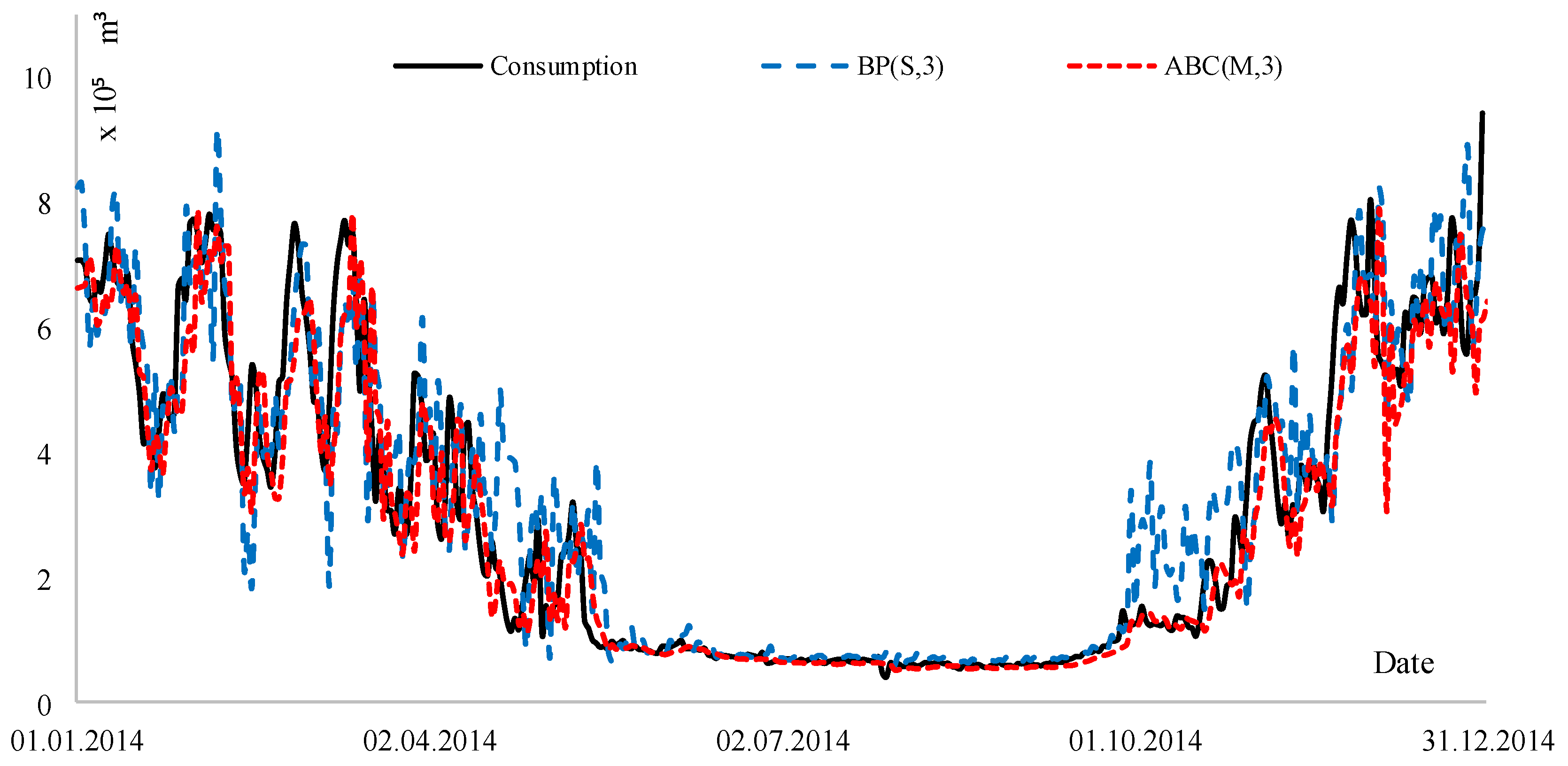
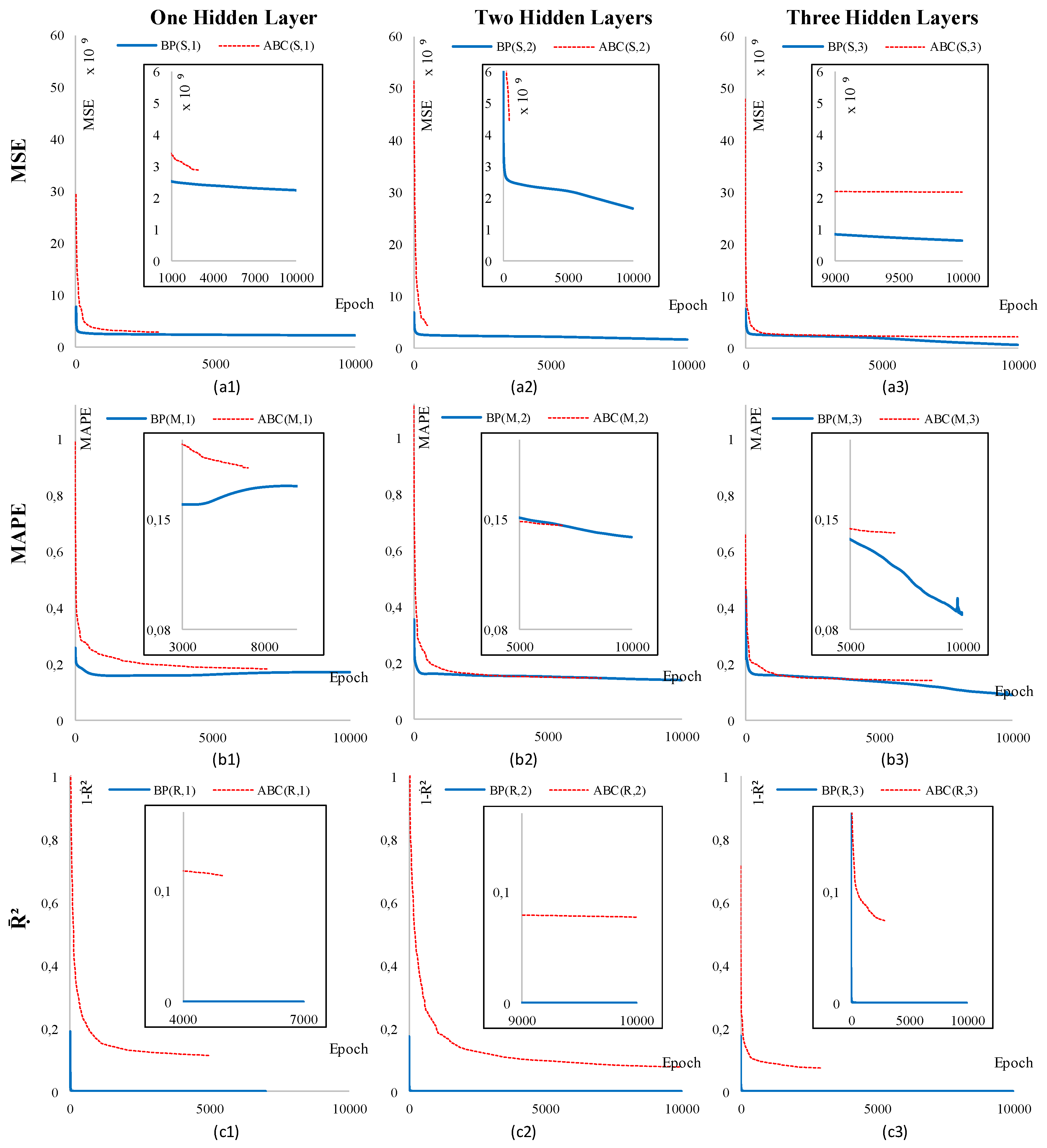
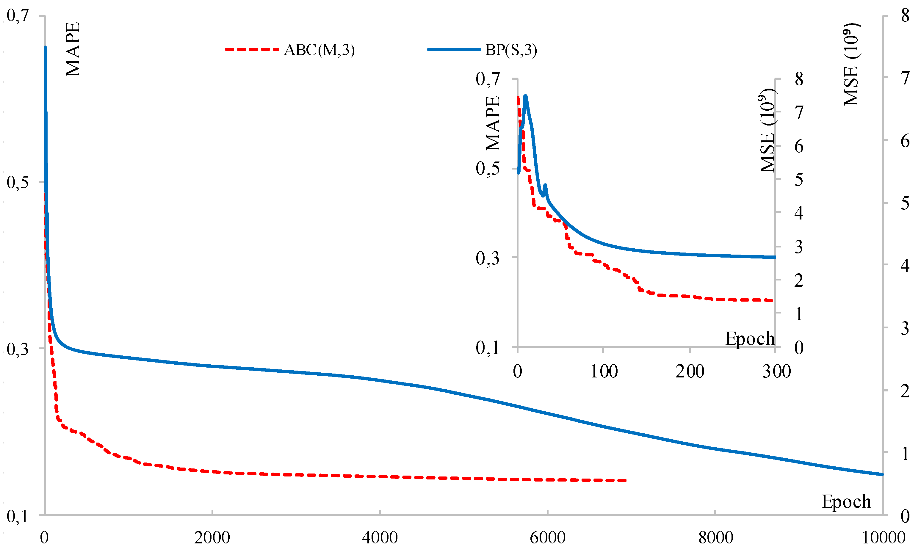
4. Scenarios and Results
5. Conclusions
Acknowledgments
Author Contributions
Conflicts of Interest
Abbreviations
| ABC | Artificial Bee Colony |
| ANFIS | Adaptive Neuro Fuzzy Inference System |
| ANN | Artificial Neural Network |
| ARIMA | Autoregressive Integrated Moving Average |
| BP | Back Propagation |
| DE | Differential Evolution |
| EMRA | Energy Market Regulatory Authority |
| FDEA | Fuzzy Data Envelopment Analysis |
| GA | Genetic Algorithm |
| LNG | Liquid Natural Gas |
| MAPE | Mean Absolute Percentage Error |
| MLP | Multi Layer Perceptron |
| MSE | Mean Squared Error |
| OLS | Ordinary Least Squares |
| PPC | Petroleum Pipeline Corporation |
| RBF | Radial Basis Functions |
| RMS | Reduction and Measuring Stations |
| SVM | Support Vector Machines |
References
- Khotanzad, A.; Elragal, H.; Lu, T.L. Combination of artificial neural-network forecasters for prediction of natural gas consumption. IEEE Trans. Neural Netw. 2000, 11, 464–473. [Google Scholar] [CrossRef] [PubMed]
- Gorucu, F.B. Artificial Neural Network Modeling for Forecasting Gas Consumption. Energy Sources 2004, 26, 299–307. [Google Scholar] [CrossRef]
- Potočnik, P.; Thaler, M.; Govekar, E.; Grabec, I.; Poredoš, A. Forecasting risks of natural gas consumption in Slovenia. Energy Policy 2007, 35, 4271–4282. [Google Scholar] [CrossRef]
- Akpinar, M.; Yumusak, N. Estimating household natural gas consumption with multiple regression: Effect of cycle. In Proceedings of the IEEE 2013 International Conference on Electronics, Computer and Computation (ICECCO), Ankara, Turkey, 7–9 November 2013; pp. 188–191. [Google Scholar]
- Sánchez-Úbeda, E.F.; Berzosa, A. Modeling and forecasting industrial end-use natural gas consumption. Energy Econ. 2007, 29, 710–742. [Google Scholar] [CrossRef]
- Yokoyama, R.; Wakui, T.; Satake, R. Prediction of energy demands using neural network with model identification by global optimization. Energy Convers. Manag. 2009, 50, 319–327. [Google Scholar] [CrossRef]
- Azadeh, A.; Asadzadeh, S.; Ghanbari, A. An adaptive network-based fuzzy inference system for short-term natural gas demand estimation: Uncertain and complex environments. Energy Policy 2010, 38, 1529–1536. [Google Scholar] [CrossRef]
- Akpinar, M.; Yumusak, N. Naïve forecasting household natural gas consumption with sliding window approach. Turk. J. Elec. Eng. Comp. Sci. 2017, 25, 30–45. [Google Scholar] [CrossRef]
- Taşpınar, F.; Çelebi, N.; Tutkun, N. Forecasting of daily natural gas consumption on regional basis in Turkey using various computational methods. Energy Build. 2013, 56, 23–31. [Google Scholar] [CrossRef]
- Karimi, H.; Dastranj, J. Artificial neural network-based genetic algorithm to predict natural gas consumption. Energy Syst. 2014, 5, 571–581. [Google Scholar] [CrossRef]
- Soldo, B.; Potočnik, P.; Šimunović, G.; Šarić, T.; Govekar, E. Improving the residential natural gas consumption forecasting models by using solar radiation. Energy Build. 2014, 69, 498–506. [Google Scholar] [CrossRef]
- Akpinar, M.; Adak, M.F.; Yumusak, N. Forecasting Natural Gas Consumption with Hybrid Neural Networks—Artificial Bee Colony. In Proceedings of the IEEE 2016 2nd International Conference on Intelligent Energy and Power Systems, Kiev, Ukraine, 7–11 June 2016; pp. 101–106. [Google Scholar]
- Adak, M.F.; Duru, N.; Duru, H.T. Elevator simulator design and estimating energy consumption of an elevator system. Energy Build. 2013, 65, 272–280. [Google Scholar] [CrossRef]
- Yao, S.; Song, Y.; Zhang, L.; Cheng, X. Wavelet transform and neural networks for short-term electrical load forecasting. Energy Convers. Manag. 2000, 41, 1975–1988. [Google Scholar] [CrossRef]
- Yalcinoz, T.; Eminoglu, U. Short term and medium term power distribution load forecasting by neural networks. Energy Convers. Manag. 2005, 46, 1393–1405. [Google Scholar] [CrossRef]
- Amjady, N. Day-Ahead Price Forecasting of Electricity Markets by a New Fuzzy Neural Network. IEEE Trans. Power Syst. 2006, 21, 887–896. [Google Scholar] [CrossRef]
- PAO, H. Comparing linear and nonlinear forecasts for Taiwan’s electricity consumption. Energy 2006, 31, 2129–2141. [Google Scholar] [CrossRef]
- Ermis, K.; Midilli, A.; Dincer, I.; Rosen, M. Artificial neural network analysis of world green energy use. Energy Policy 2007, 35, 1731–1743. [Google Scholar] [CrossRef]
- Sözen, A.; Arcaklioglu, E. Prediction of net energy consumption based on economic indicators (GNP and GDP) in Turkey. Energy Policy 2007, 35, 4981–4992. [Google Scholar] [CrossRef]
- Hamzaçebi, C. Forecasting of Turkey’s net electricity energy consumption on sectoral bases. Energy Policy 2007, 35, 2009–2016. [Google Scholar] [CrossRef]
- Tso, G.K.; Yau, K.K. Predicting electricity energy consumption: A comparison of regression analysis, decision tree and neural networks. Energy 2007, 32, 1761–1768. [Google Scholar] [CrossRef]
- González-Romera, E.; Jaramillo-Morán, M.; Carmona-Fernández, D. Monthly electric energy demand forecasting with neural networks and Fourier series. Energy Convers. Manag. 2008, 49, 3135–3142. [Google Scholar] [CrossRef]
- Azadeh, A.; Ghaderi, S.; Sohrabkhani, S. Annual electricity consumption forecasting by neural network in high energy consuming industrial sectors. Energy Convers. Manag. 2008, 49, 2272–2278. [Google Scholar] [CrossRef]
- Ying, L.C.; Pan, M.C. Using adaptive network based fuzzy inference system to forecast regional electricity loads. Energy Convers. Manag. 2008, 49, 205–211. [Google Scholar] [CrossRef]
- Saini, L.M. Peak load forecasting using Bayesian regularization, Resilient and adaptive backpropagation learning based artificial neural networks. Electr. Power Syst. Res. 2008, 78, 1302–1310. [Google Scholar] [CrossRef]
- Pao, H. Forecasting energy consumption in Taiwan using hybrid nonlinear models. Energy 2009, 34, 1438–1446. [Google Scholar] [CrossRef]
- Geem, Z.W.; Roper, W.E. Energy demand estimation of South Korea using artificial neural network. Energy Policy 2009, 37, 4049–4054. [Google Scholar] [CrossRef]
- Sözen, A. Future projection of the energy dependency of Turkey using artificial neural network. Energy Policy 2009, 37, 4827–4833. [Google Scholar] [CrossRef]
- Kankal, M.; Akpınar, A.; Kömürcü, M.h.; Özşahin, T.ü. Modeling and forecasting of Turkey’s energy consumption using socio-economic and demographic variables. Appl. Energy 2011, 88, 1927–1939. [Google Scholar] [CrossRef]
- Azadeh, A.; Saberi, M.; Asadzadeh, S.M.; Hussain, O.K.; Saberi, Z. A neuro-fuzzy-multivariate algorithm for accurate gas consumption estimation in South America with noisy inputs. Int. J. Electr. Power Energy Syst. 2013, 46, 315–325. [Google Scholar] [CrossRef]
- Szoplik, J. Forecasting of natural gas consumption with artificial neural networks. Energy 2015, 85, 208–220. [Google Scholar] [CrossRef]
- Azadeh, A.; Asadzadeh, S.; Mirseraji, G.; Saberi, M. An emotional learning-neuro-fuzzy inference approach for optimum training and forecasting of gas consumption estimation models with cognitive data. Technol. Forecast. Soc. Chang. 2015, 91, 47–63. [Google Scholar] [CrossRef]
- Uzlu, E.; Akpınar, A.; Özturk, H.T.; Nacar, S.; Kankal, M. Estimates of hydroelectric generation using neural networks with the artificial bee colony algorithm for Turkey. Energy 2014, 69, 638–647. [Google Scholar] [CrossRef]
- Li, Y.; Wang, Y.; Li, B. A hybrid artificial bee colony assisted differential evolution algorithm for optimal reactive power flow. Int. J. Electr. Power Energy Syst. 2013, 52, 25–33. [Google Scholar] [CrossRef]
- Adak, M.; Yumusak, N. Classification of E-Nose Aroma Data of Four Fruit Types by ABC-Based Neural Network. Sensors 2016, 16, 304. [Google Scholar] [CrossRef] [PubMed]
- Suganthi, L.; Samuel, A.A. Energy models for demand forecasting—A review. Renew. Sustain. Energy Rev. 2012, 16, 1223–1240. [Google Scholar] [CrossRef]
- Soldo, B. Forecasting natural gas consumption. Appl. Energy 2012, 92, 26–37. [Google Scholar] [CrossRef]
- Karaboga, D.; Gorkemli, B.; Ozturk, C.; Karaboga, N. A comprehensive survey: Artificial bee colony (ABC) algorithm and applications. Artif. Intell. Rev. 2014, 42, 21–57. [Google Scholar] [CrossRef]
- BOTAS. Iletim Sebekesi Isleyis Duzenlemelerine Iliskin Esaslar (The Basis of Regulatory Process on Transmission Network); The Official Gazette of the Turkish Republic: Ankara, Turkey, 2013. [Google Scholar]
- Energy Market Regulatory Authority. Turkish Natural Gas Market Report 2014; Technical report; Energy Market Regulatory Authority: Ankara, Turkey, 2015.
- Akpinar, M.; Yumusak, N. Year Ahead Demand Forecast of City Natural Gas Using Seasonal Time Series Methods. Energies 2016, 9, 727. [Google Scholar] [CrossRef]
- Zhang, G. Time series forecasting using a hybrid ARIMA and neural network model. Neurocomputing 2003, 50, 159–175. [Google Scholar] [CrossRef]
- Chen, T. Estimating job cycle time in a wafer fabrication factory: A novel and effective approach based on post-classification. Appl. Soft Comput. 2016, 40, 558–568. [Google Scholar] [CrossRef]
- Schalkoff, R.J. Artificial Neural Networks, 1st ed.; McGraw Hill: New York, NY, USA, 1997. [Google Scholar]
- Karaboga, D. An Idea Based on Honey Bee Swarm for Numerical Optimization; Technical Report TR06; Erciyes University: Kayseri, Turkey, 2005; p. 10. [Google Scholar]
- Bishop, C. Pattern Recognition and Machine Learning, 1st ed.; Springer-Verlag: New York, NY, USA, 2006; p. 738. [Google Scholar]
- Vasant, P.M. Meta-Heuristics Optimization Algorithms in Engineering, Business, Economics, and Finance; IGI Global: Hershey, PA, USA, 2013; p. 734. [Google Scholar]


| Descriptive Statistics | C | ||
|---|---|---|---|
| Mean | 290,914 | 0.28 | 0.32 |
| Standard Error | 6604 | 0.01 | 0.01 |
| Median | 202,069 | 0.18 | 0.25 |
| Mode | 45,254 | 0.02 | 0.11 |
| Standard Deviation | 252,417 | 0.27 | 0.21 |
| Sample Variance | 63,714,170,871 | 0.07 | 0.05 |
| Kurtosis | −0.90 | −0.90 | −0.90 |
| Skewness | 0.65 | 0.65 | 0.65 |
| Range | 947,195 | 1.00 | 0.80 |
| Minimum | 27,765 | 0.00 | 0.10 |
| Maximum | 974,960 | 1.00 | 0.90 |
| Sum | 425,025,317 | 405.89 | 470.82 |
| Count | 1461 | 1461 | 1461 |
| Parameter (ABC) | Value | Parameter (BP) | Value |
|---|---|---|---|
| Lower bound | −10 | Learning rate | 0.2 |
| Upper bound | 10 | Momentum | 0.8 |
| Colony size | 100 | Weights’ lower bound | −1 |
| Food source limit | 365 | Weights’ upper bound | 1 |
| Hidden Layer Epochs | 500 | 1000 | 3000 | 5000 | 7000 | 10,000 |
|---|---|---|---|---|---|---|
| One Hidden Layer | 5 | 5 | 5 | 5 | 5 | 5 |
| Two Hidden Layers | 6 | 12 | 6 | 12 | 18 | 6 |
| Three Hidden Layers | - | - | 3 | 3 | 12 | 9 |
| Types of Structures | MSE | MAPE | |||||
|---|---|---|---|---|---|---|---|
| BP | ABC | BP | ABC | BP | ABC | ||
| One hidden layer | Neurons/Epochs | 40/ | 20/3 × | 20/ | 20/7 × | 20/7 × | 40/5 × |
| Abbreviation | BP(S,1) | ABC(S,1) | BP(M,1) | ABC(M,1) | BP(R,1) | ABC(R,1) | |
| Two hidden layers | Neurons/Epochs | 20 + 50/ | 20 + 40/500 | 20 + 30/ | 20 + 20/7 × | 20 + 60/ | 20 + 60/ |
| Abbreviation | BP(S,2) | ABC(S,2) | BP(M,2) | ABC(M,2) | BP(R,2) | ABC(R,2) | |
| Three hidden layers | Neurons/Epochs | 20 + 60 + 15/ | 20 + 10 + 15/ | 20 + 60 + 30/ | 20 + 10 + 5/7 × | 20 + 60 + 30/ | 20 + 10 + 5/3 × |
| Abbreviation | BP(S,3) | ABC(S,3) | BP(M,3) | ABC(M,3) | BP(R,3) | ABC(R,3) | |
| Training Type | One Layer | Two Layers | Three Layers | ||||
|---|---|---|---|---|---|---|---|
| BP | ABC | BP | ABC | BP | ABC | ||
| MSE | Model | BP(S,1) | ABC(S,1) | BP(S,2) | ABC(S,2) | BP(S,3) | ABC(S,3) |
| MAPE | 99.2% | 16.4% | 63.8% | 17.6% | 30.2% | 16.9% | |
| MAPE | Model | BP(M,1) | ABC(M,1) | BP(M,2) | ABC(M,2) | BP(M,3) | ABC(M,3) |
| MAPE | 99.9% | 16.3% | 61.7% | 15.4% | 33.9% | 14.9% | |
| Model | BP(R,1) | ABC(R,1) | BP(R,2) | ABC(R,2) | BP(R,3) | ABC(R,3) | |
| MAPE | 97.6% | 17.8% | 63.5% | 17.4% | 34.3% | 18.0% | |
© 2017 by the authors. Licensee MDPI, Basel, Switzerland. This article is an open access article distributed under the terms and conditions of the Creative Commons Attribution (CC BY) license (http://creativecommons.org/licenses/by/4.0/).
Share and Cite
Akpinar, M.; Adak, M.F.; Yumusak, N. Day-Ahead Natural Gas Demand Forecasting Using Optimized ABC-Based Neural Network with Sliding Window Technique: The Case Study of Regional Basis in Turkey. Energies 2017, 10, 781. https://doi.org/10.3390/en10060781
Akpinar M, Adak MF, Yumusak N. Day-Ahead Natural Gas Demand Forecasting Using Optimized ABC-Based Neural Network with Sliding Window Technique: The Case Study of Regional Basis in Turkey. Energies. 2017; 10(6):781. https://doi.org/10.3390/en10060781
Chicago/Turabian StyleAkpinar, Mustafa, M. Fatih Adak, and Nejat Yumusak. 2017. "Day-Ahead Natural Gas Demand Forecasting Using Optimized ABC-Based Neural Network with Sliding Window Technique: The Case Study of Regional Basis in Turkey" Energies 10, no. 6: 781. https://doi.org/10.3390/en10060781
APA StyleAkpinar, M., Adak, M. F., & Yumusak, N. (2017). Day-Ahead Natural Gas Demand Forecasting Using Optimized ABC-Based Neural Network with Sliding Window Technique: The Case Study of Regional Basis in Turkey. Energies, 10(6), 781. https://doi.org/10.3390/en10060781