Article

Design Optimization of a High Power LED Matrix Luminaire

by
Jose Luiz F. Barbosa
1,2,*,‡,†,
Dan Simon
3,‡ and
Wesley P. Calixto
1,2,‡
1
Experimental & Technological Research and Study Group (NExT), Federal Institute of Goias, Goiania, GO 74055-110, Brazil
2
School of Electrical, Mechanical and Computer Engineering, Federal University of Goias, Goiania, GO 74605-010, Brazil
3
Department of Electrical Engineering and Computer Science, Cleveland State University, Cleveland, OH 44115, USA
*
Author to whom correspondence should be addressed.
This paper is an extended version of our paper published in Selected Papers from 16 IEEE International Conference on Environment and Electrical Engineering (EEEIC Florence Italy 6 June 2016).
These authors contributed equally to this work.
Energies 2017, 10(5), 639; https://doi.org/10.3390/en10050639
Submission received: 16 February 2017 / Revised: 5 April 2017 / Accepted: 6 April 2017 / Published: 5 May 2017

Abstract

:
This work presents a methodology for optimizing the layout and geometry of an m × n high power (HP) light emitting diode (LED) luminaire. Two simulators are used to analyze an LED luminaire model. The first simulator uses the finite element method (FEM) to analyze the thermal dissipation, and the second simulator uses the ray tracing method for lighting analysis. The thermal and lighting analysis of the luminaire model is validated with an error of less than 10%. The goal of the optimization process is to find a solution that satisfies both thermal dissipation and light efficiency. The optimization goal is to keep the LED temperature at an acceptable level while still obtaining uniform illumination on a target plane. Even though no optical accessories or active cooling systems are used in the model, the results demonstrate that it is possible to obtain satisfactory results even with a limited number of parameters. The optimization results show that it is possible to design luminaires with 4, 6 and up to 8 HP-LEDs, keeping the LED temperature at about 100 C. However, the best uniformity on a target plane was found by the heuristic algorithm.

1. Introduction

Artificial lighting is essential to the quality of life in human society. It allows business and leisure activities and promotes a sense of personal security in the absence of natural light. Indoor artificial lighting applies to homes, businesses and industry. Outdoor artificial lighting applies to sidewalks, streets, roads, bridges, tunnels, parking lots, monuments and building facades and usually is called street lighting [1,2].
Concerns about the electricity consumption spent on artificial lighting is growing [3]. About 20% of all electricity generated in the world is used for illumination, and the need to manage energy consumption is an important priority [4,5,6].
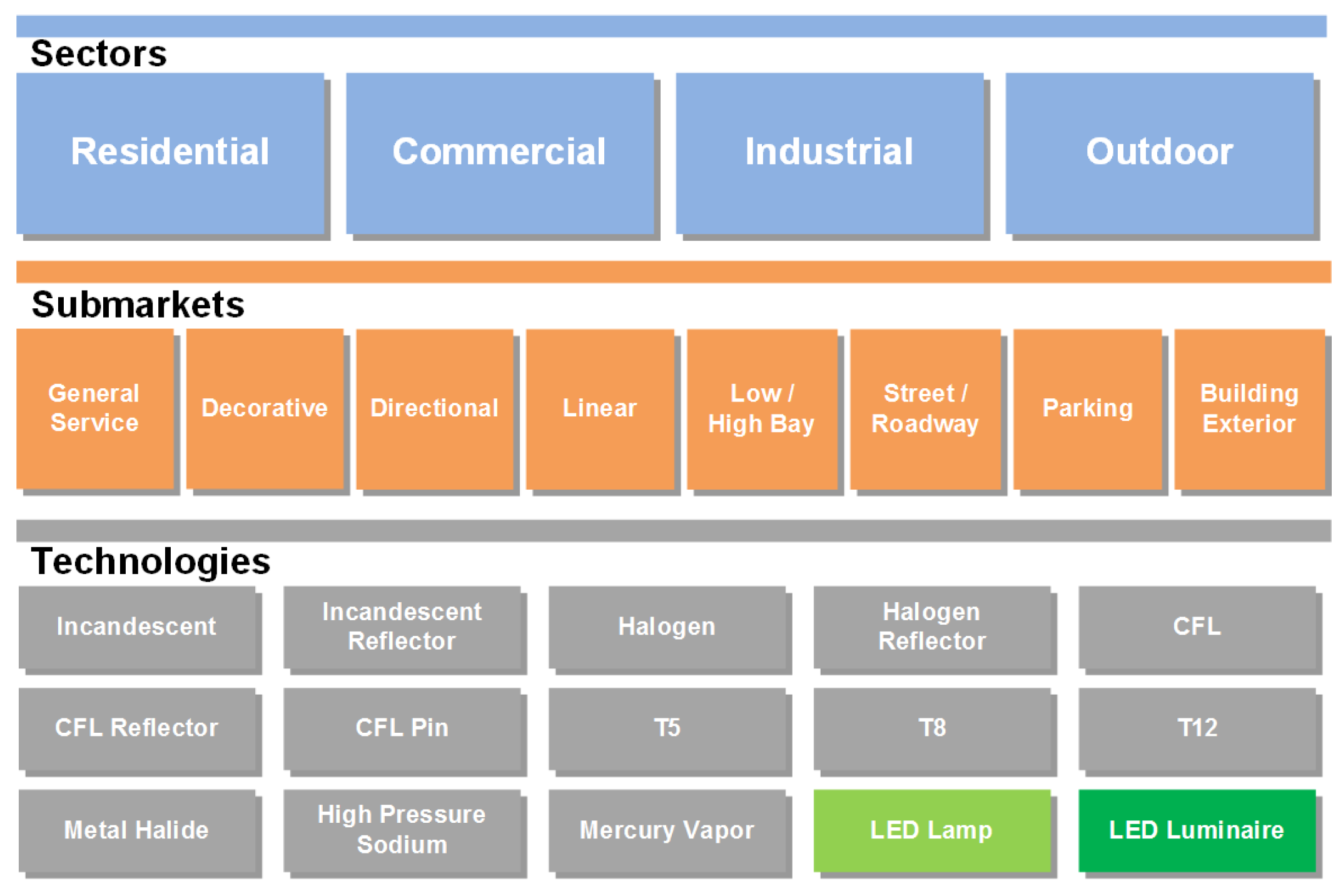
The current U.S. lighting market model is composed of four sectors that are divided into eight sub-markets and a total of 15 technology categories, as represented in Figure 1. The outdoor lighting sector includes the following sub-markets: street and roadway, parking and exterior building [1].
The 10 largest U.S. metropolitan areas include 4.4 million street lights with an estimated annual consumption of three billion kWh and the equivalent production of 2.3 million metric tons of CO 2 , according to reports from 2008 [7]. The Bureau of Energy Efficiency used statistics from the Central Electricity Authority to estimate a gross energy consumption of 6.131 million kWh of street lighting in Portugal from 2007 to 2008 [8].
Data from 2005 show an estimated consumption of 35 TWh in street lighting in the 25 European Union countries (EU25), which represents about 1.3% of the total electricity consumption of that region [9]. Data from 2006 show about nine million street lighting points in Germany for 82 million people. An extrapolation over Europe based on this ratio of 0.11 luminaires/capita results in an estimate of 91 million street lighting points in Europe (with 820 million inhabitants) [9]. According to research from 2008, there are about 15 million street lighting points in Brazil [10].
City lighting management is changing due to impacts on both economics and on the environment. The economic resources of governments are becoming increasingly limited due to the slowdown of the world economy, but electricity prices continue to increase. Maintenance costs are also increasing, with a large number of lamps approaching the end of their life [7].
High power (HP)-LEDs have several advantages compared to traditional lighting sources, such as: (i) long life; (ii) high brightness; (iii) low power consumption; (iv) compact size; (v) fast response; (vi) high reliability [2,4,6,11]; and (vii) mechanical shock and vibration resistance [12].
LED lamps and LED luminaires have a high cost compared to other lighting technologies and are therefore restricted to a few generic lighting applications. However, according to predictions from the U.S. lighting market model in the street and roadway sub-market, LEDs will reach 83% market share by 2020 and approximately 100% by 2030 ([1]).
Energy savings includes a corresponding CO 2 reduction. A savings of 1500 kWh reduces CO 2 emissions by about one ton [7]. In Japan, it is estimated that the adoption of a street lighting system based on LED lamps could reduce the emission of CO 2 by six to nine million tons each year [13].
However, there are difficulties in using HP-LEDs in outdoor lighting, such as: thermal dissipation (which can degrade luminous efficacy), optical performance (including optical efficiency) and the shape of the area to be illuminated [14]. There are only a few studies that present a performance evaluation of the installation of outdoor LED luminaires [15]. These difficulties are a challenge in the design of HP-LED outdoor lighting [16].
Good LED thermal management should ensure that LED lifetime is not prematurely degraded and should maximize optical performance and allow operation at the maximum allowable current within the allowable temperature range [17,18]. Although various thermal devices can be used for thermal dissipation, they can generally be divided into two categories: passive and active. Passive thermal management refers to technologies that rely exclusively on the thermodynamics of conduction, convection and radiation, such as heat sinks [19]. Active thermal management refers to cooling technologies that introduce external energy, usually from an external device, to increase heat transfer. Usually, when active systems are used, they are augmented with passive systems [20,21].
Some papers present a reliability evaluation of LEDs’ reliability and the temperature influence on LED parameters, such as MTTR (mean time to repair) and MTBF (mean time between failure) [22,
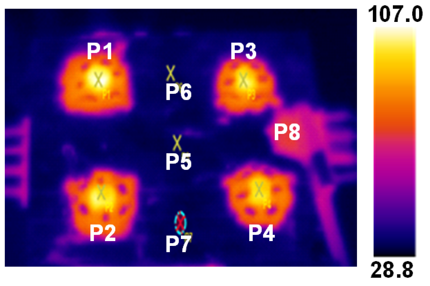
23]. The junction temperature of the LED can be estimated by some techniques. It can be calculated from the temperature of the LED module and the thermal resistance of the LED junction (obtained in the manufacturer’s datasheet); calculated by shifting the direct voltage changes over the component; and direct measurements of the temperature of the LED via thermocouple or infrared images [24]. There are many works that present analyses of thermal dissipation of HP-LED lamps and luminaires using finite element method (FEM) software [25,26,27,28,29]. A thermal and luminous analysis of a luminaire composed of three LEDs of 1 W is presented in [30]; however, there are not many works that evaluate the thermal heat dissipation and also the illumination quality generated by an HP-LED luminaire.
This work is an extended version of the conference paper [31] and presents studies that can enable the design of an optimal HP-LED luminaire, which is technically and economically feasible. The HP-LED luminaire model in this paper includes six parameters that affect heat dissipation and lighting efficiency. The design problem is therefore a multi-objective problem: find the best design with respect to both thermal management and illuminated target area. Only one heat sink is used as a heat exchanger in this paper (passive system). In the Methodology section, the techniques involved in two simulators used in the multi-objective problem solution are approached. In model validation, the proposed model is shown, the simulators configured and the validation presented. In the Optimization section, an evaluation function for the problem is proposed. In the Results section, two case studies using deterministic optimization are included as a comparison with previously-published heuristic optimization results [31].

2. Methodology

Modeling and simulation allow for the representation of a physical system or process in a shorter time and at a lower cost than experimentation. In many cases, models are too complex for a formal mathematical analysis (analytical solution), and so, numerical methods are used with computational tools for the simulation. After a model is tested and validated, new conditions can be simulated and evaluated. This process reduces the number of physical tests that are required, which reduces engineering time and minimizes damage to the physical components [14].
A model that can represent the HP-LED luminaire is presented here in terms of both its physics and its constraints in order to allow the simulation of heat dissipation and the lighting on a target plane.

2.1. Thermal Management

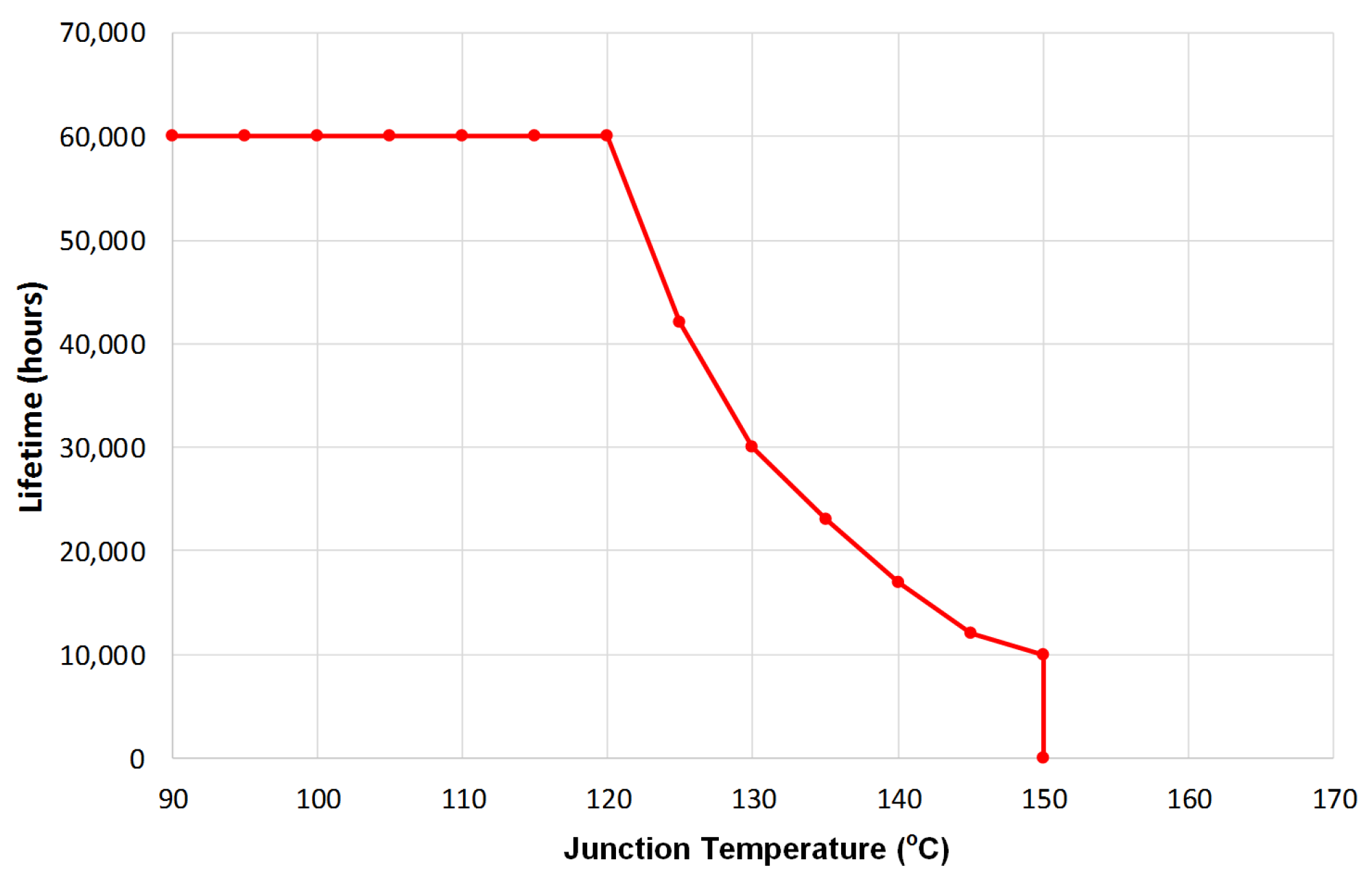
The first problem discussed here is the LED luminaire operating temperature. HP-LED lifetime is associated with operating temperature, and lifetime can be drastically reduced under high temperatures. Figure 2 illustrates the relationship between junction temperature and the lifetime of an HP-LED with maximum continuous forward current. It can be seen that the junction temperature of the LED should be maintained below 120 C.
Finite element method (FEM) software (COMSOL Multiphysics, version 5.2) is used to model the physical laws that describe the heat exchange. The thermal analysis is performed using the Heat Transfer Solid module from COMSOL [32].
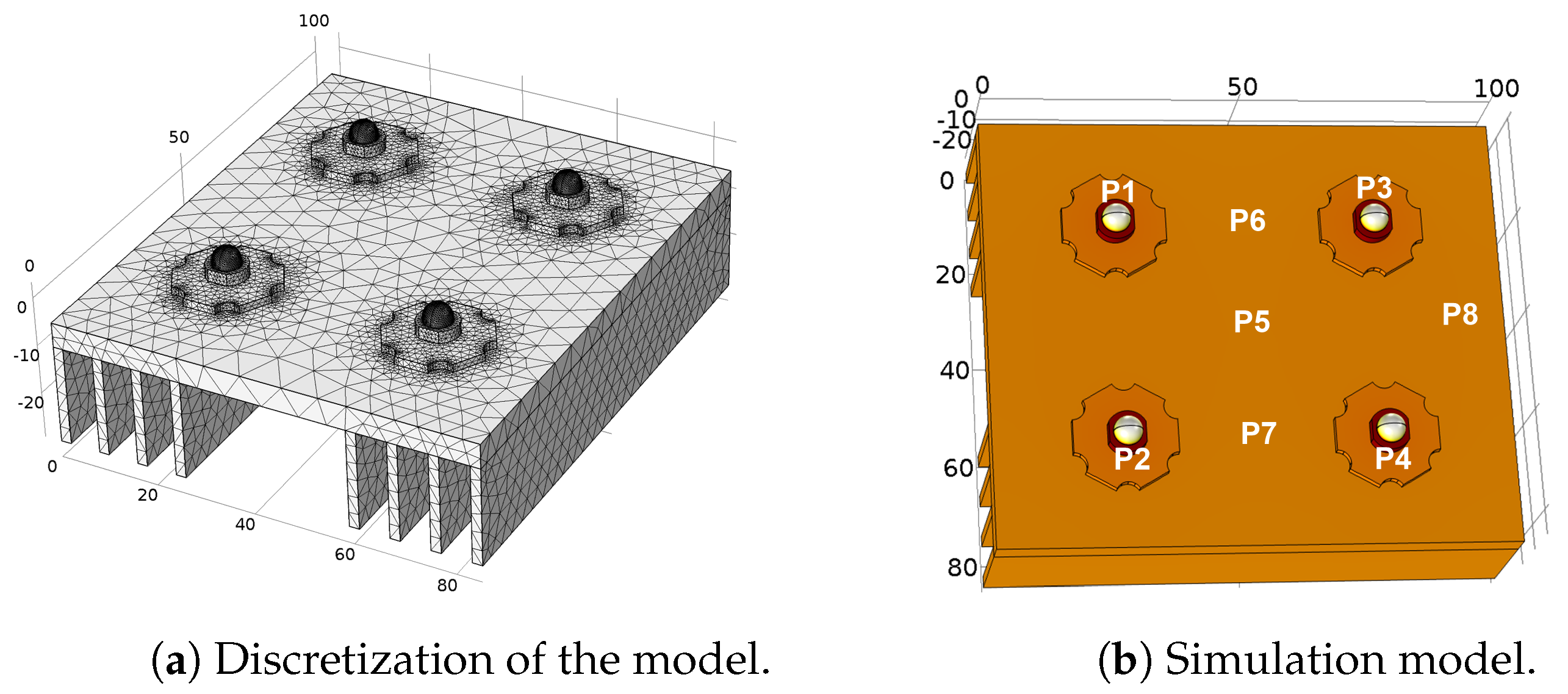
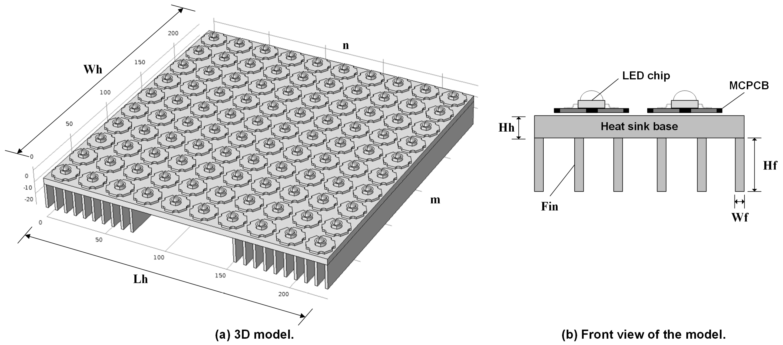
A 3D CAD model of the LED is designed and exported to COMSOL. Other geometries ((MCPCB) and heat sink base with fins) are designed directly in COMSOL. The simplification of the model can provide a clear thermal path in order to access the thermal performance from heat source to the heat sink; therefore, the electrical connection (wire and connector) was not modeled. The model and its parameters are illustrated in Figure 3a,b. Table 1 shows the thermal conductivities of the materials used in the model.
The mesh element number is increased until it reaches grid independence during the thermal simulation. As the geometry of the luminaire is dynamic, i.e., the heat sink dimensions and the number of LEDs vary, the number of elements in the mesh depends on the geometry of the object being simulated.
Therefore, the maximum mesh element size ( H E S M max ) is set to 10% of the heat sink width ( W h ) and the minimum element size ( H E S M min ) as 18% of H E S M max . For the LED object (composed of the chip and MCPCB), as it has a fixed geometry, the maximum mesh element size ( L E S M max ) is set to 5 mm and the minimum element size ( L E S M min ) as 0.4 mm. Both proportions found came from empirical tests.
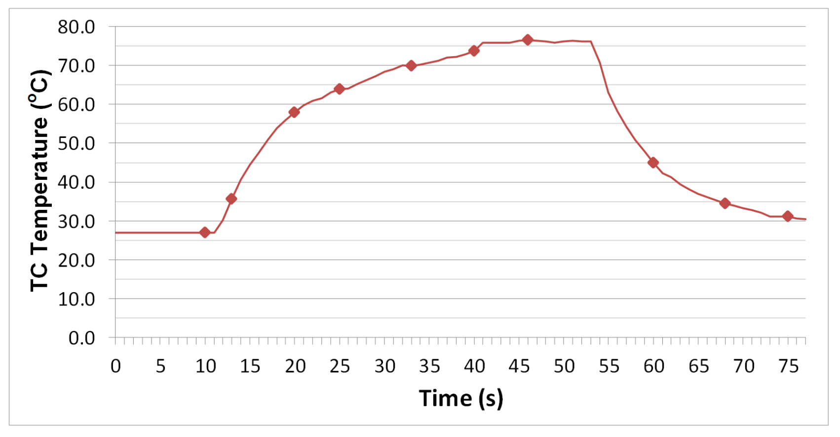
The boundary condition of the simulation model is defined as a room temperature ( T 0 ) of 27.2 C, and a heat coefficient value of 5 W/(m 2 · K) is used for heat transfer from the heat sink to air (natural convection). The LED chip is the only heat source with a uniform plane surface, and its input power ( P L E D ) is 5 W each one. The modeling structure is perfectly interfaced. A list of global parameters that affect the model is given in Table 2.

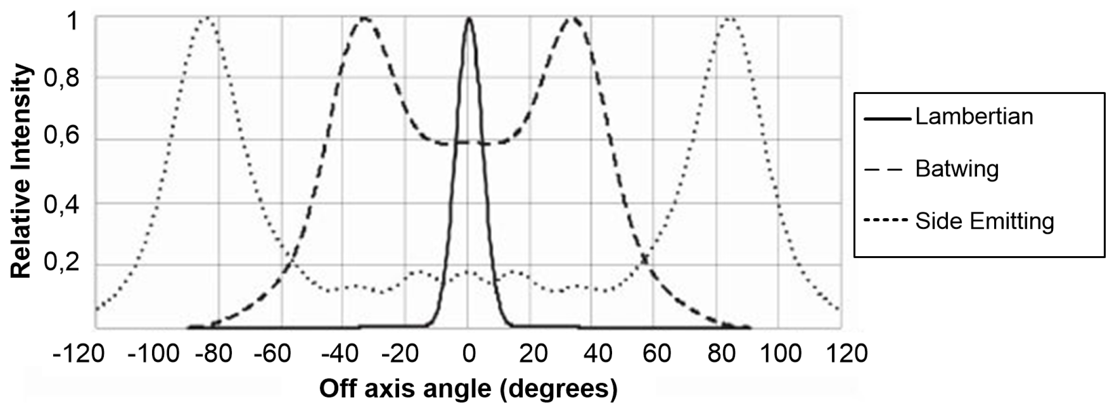
2.2. LED Radiation Pattern

The second problem discussed is the LED radiation pattern. HP-LEDs do not emit the same luminous flux in all directions. The luminous polar diagram in Figure 4 shows three typical radiation patterns: Lambertian, bat wing and side-emitting.
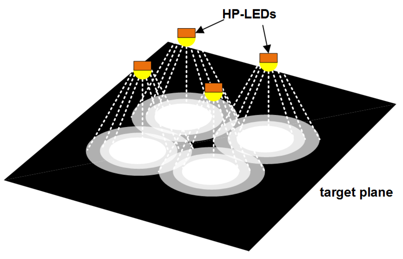
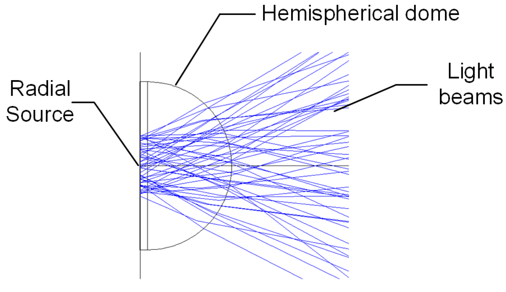
A numerical technique called ray tracing, which is based on the Snell–Descartes law, is used for lighting simulation. The HP-LED luminaire model is designed in the optical simulation software. The high-level simulation includes a stochastic simulation of about one million light rays emitted by each LED, and the extraction of the luminous pattern from the target plane. This process is illustrated in Figure 5.

3. Model Validation

3.1. Thermal Modeling and Simulation

The HP-LED luminaire model includes four 5-W LEDs (a 2 × 2 array) attached to an aluminum heat sink base of 100 m m × 85 m m × 25 m m (width × length × height). The geometric parameters are adjusted, and a model mesh is generated by the FEM software as illustrated in Figure 6a. The complete mesh for this geometry consists of 90,846 tetrahedral elements, 32,148 boundary elements and 3548 edge elements.
Figure 6b shows the HP-LED luminaire thermal dissipation model after it is simulated. In this work, the LED temperature is defined as the maximum temperature that the LED chip reaches.
The simulated steady-state temperatures of the HP-LED luminaire were collected at points P1 to P8 as illustrated in Figure 6b and are shown in Table 3.

3.2. Experimental Thermal Test

An HP-LED luminaire is built with the same geometry and dimensions as the simulated model to validate the simulation. Figure 7 illustrates the four HP-LEDs attached on an aluminum heat sink base.
This prototype uses four Model W 081 F - 5 W 5-W LEDs with nominal current and voltage of 720 mA and 7 V, respectively, maximum luminous flux of Φ of 250 lm and a Lambertian radiation pattern. The LED leads are welded into a MCPCB, and a thermal paste is applied between the base of the LED and the base.
Initial tests are performed with the nominal LED supply voltage of 7 V and room temperature 27.2 C. A thermocouple (TC) is attached to the heat sink base and connected to a computer to measure and record the temperature, as illustrated in Figure 8. After 55 min, the power source of the luminaire is turned off.
A laser thermal camera is used as an auxiliary sensor to collect temperature data. Throughout the process, data are collected 10 times, represented by the markers highlighted in Figure 8. Figure 9 illustrates the HP-LED luminaire as recorded by the laser thermal camera after 40 min, which is steady state.
The temperature values of the HP-LED luminaire in the steady state, collected with both techniques, are shown in Table 4.
Surfaces with an emissivity less than 0.60 result in unreliable and inconsistent temperature determination. The lower the emissivity, the more error associated with the temperature measurement. The heat sink temperature difference between the thermocouple and the thermal camera (on test points P5, P6 and P7) can be credited to the aluminum emissivity of the measurement, whereas on test point P8, there is a black tape used to fix the TC. Therefore, the temperature values on test points P5, P6 and P7 are rejected. For comparison purposes, the experimental temperature of the LEDs (average on test points P1, P2, P3 and P4) is 103.9 C, and the experimental temperature of the heat sink (on test point P8) is 76.3 C.
The LED temperature results obtained in the simulation (Table 3) differ by 7 . 5 % on average from the experimentally-measured results, as shown in Table 5. The LED chip temperature reaches 111.7 C in the simulation and 103.9 C (on average) in the experiment. This difference of about 7.8 C can be credited to electrical losses (reduction of the LED nominal power) and the accuracy of the simulated measurement, which is collected directly at the LED chip. The heat sink temperature reached an average of 76.7 C in the simulation and 76.3 C in the experiment. Therefore, the thermal dissipation analysis model can be considered valid.

3.3. Experimental Lighting Test

The simulation was performed using ray tracing simulation software. LED modeling must be performed in non-sequential mode. In this way, at least three objects must be defined: source, geometry and detector. The source object defines the type of source that will originate the rays. The geometry object is the optical components (confinement, primary LED lens, etc.). Both are shown in Figure 10. Finally, there is detector object (target plane) that detects the rays that collide there and provides quantitative data, such as illuminance, irradiance, luminous flux, etc. Most objects are parametric, that is they are based on basic equations defined by parameters. These objects can be modified through their parameters present in an NSCE (non-sequential component editor). In the configuration of the source object, the radial type allows the luminous intensity for each angle to be set from the normal straight line to the target plane. This information, as well as other nominal LED data (power, dimensions and material used in manufacturing) are required for the simulation and can be found in the LED datasheet.
In [33], an HP-LED lamp was simulated with one 5-W LED and was experimentally validated with an error of less than 10%, as shown in Figure 11. The same setup parameters were used and replicated in the m × n HP-LED luminaire model in the present work.

4. Optimization

The optimization goal is to find luminaire parameters that provide satisfactory results in both analyses; that is, the luminaire should meet the thermal dissipation requirement that the LED junction temperature be maintained below 120 C and should provide homogeneous illumination on a target plane.
Some parameters of the luminaire were selected directly on the basis of their influence on heat dissipation. These parameters include the number of LEDs in the luminaire and the heat sink dimensions (width, length, height and number of fins). If the optimization goal was only to minimize the LED temperature, an obvious solution would be a luminaire with the fewest number of LEDs arranged in the largest possible heat sink area. This is because the smaller the number of LEDs in the luminaire, the less heat that will be created.
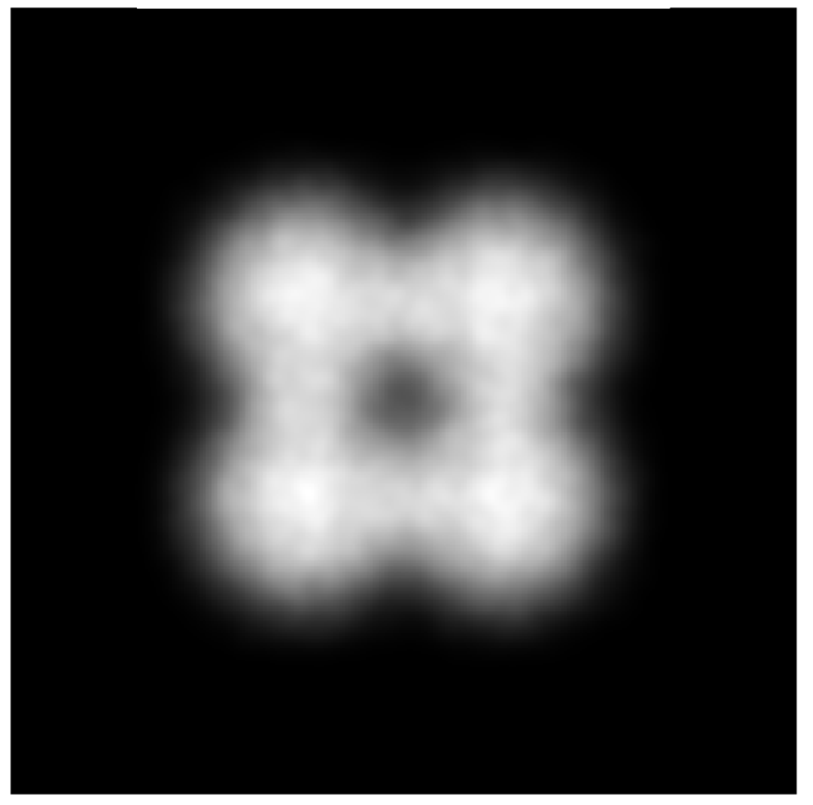
However, the number of LEDs and their layout on the luminaire directly affect the distribution of luminous flux on the target plane. A luminance simulation on a target plane of 2000 mm × 2000 mm produced by the HP-LED luminaire with four LEDs is illustrated in Figure 12. Four lighting points corresponding to the four LED luminaire sources are seen in Figure 12.
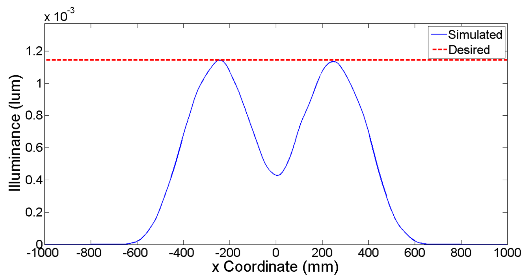
By drawing a horizontal cut line across the center of Figure 12, it is possible to plot the illuminance values as a function of the x-coordinates of the target plane in a 2D graph, as illustrated in Figure 13.

4.1. Evaluation Function

The simulation of an LED lighting application involves non-sequential ray tracing; that is, rays are randomly emitted by the source, and so, the temporal order of the ray intersections on the target surface is also random. This results in varying optical values, like illuminance E, from one simulation to the next, even when the simulation parameters are constant.
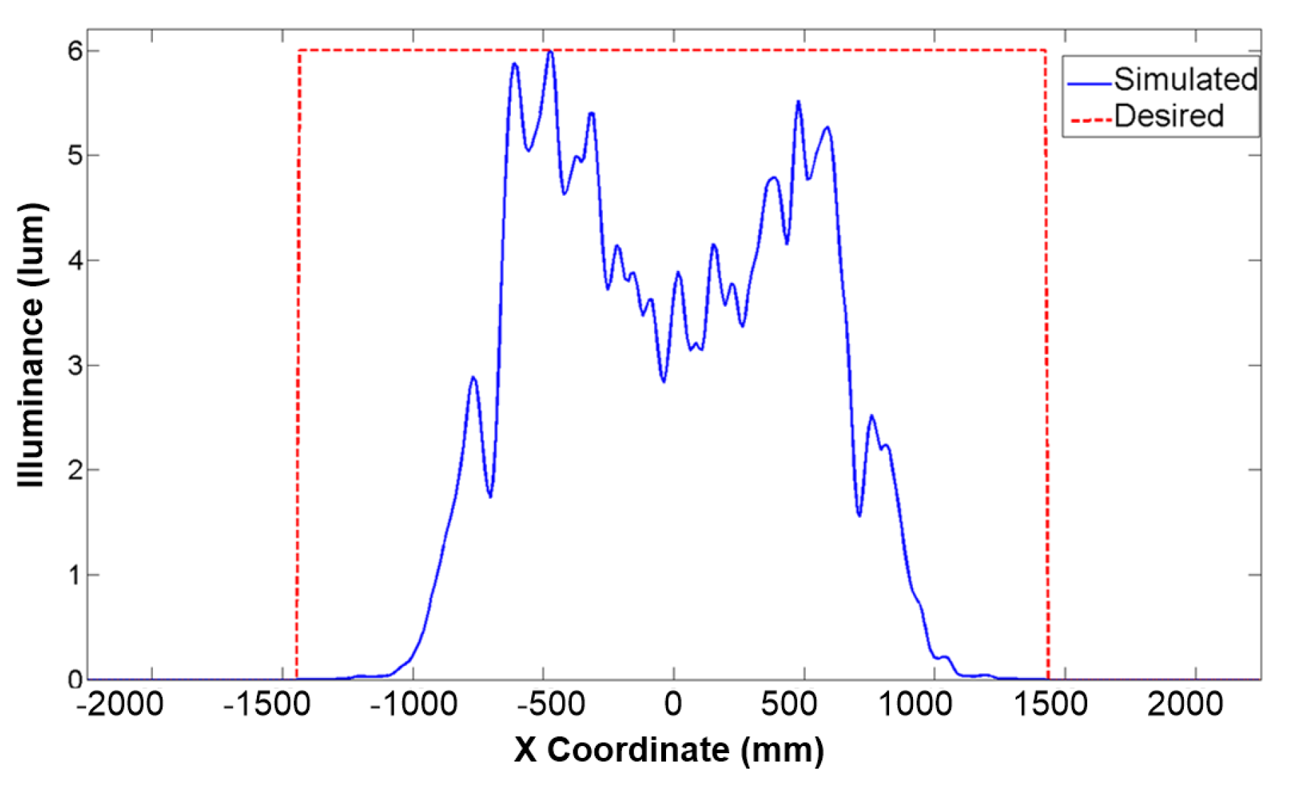
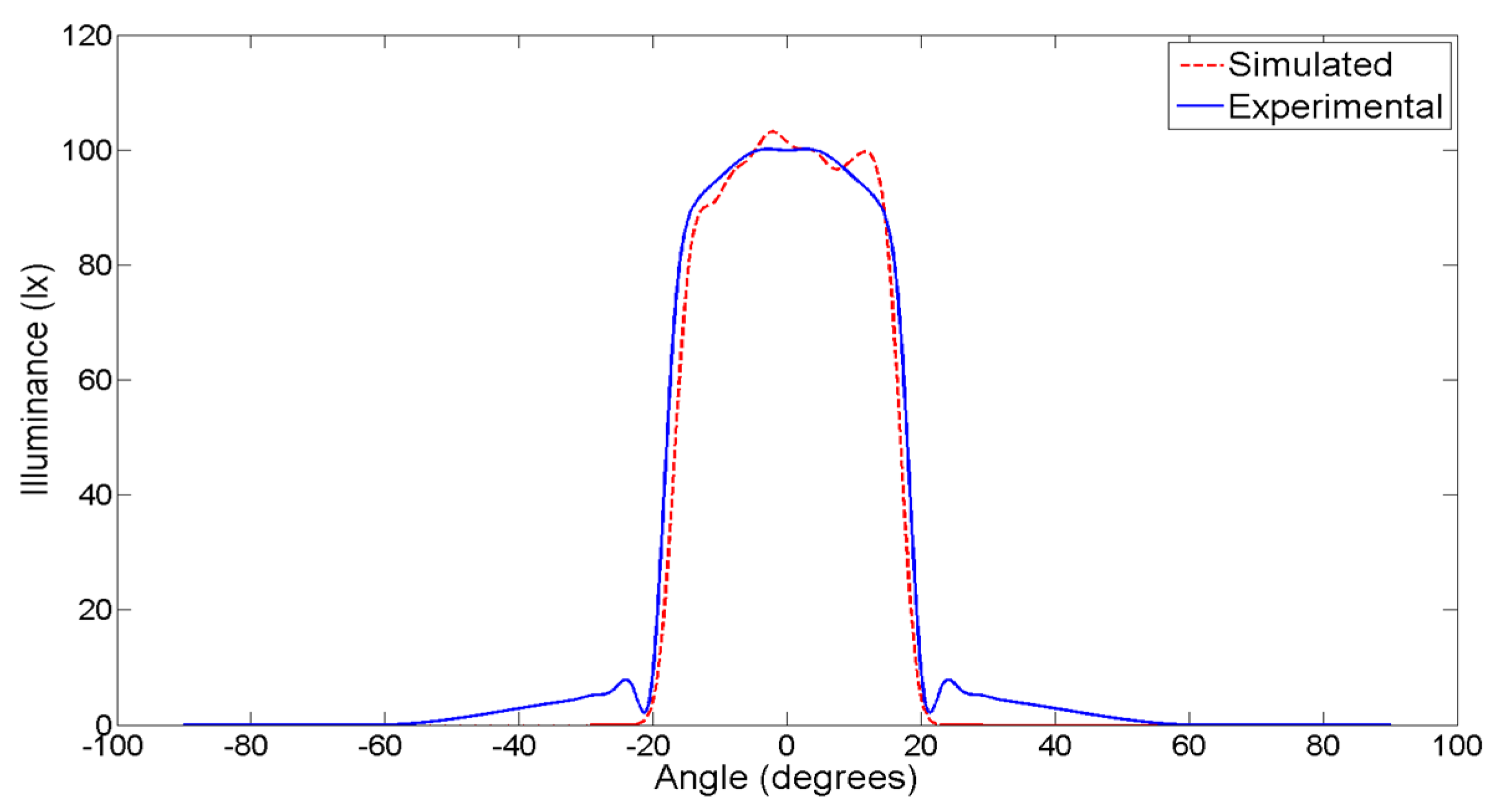
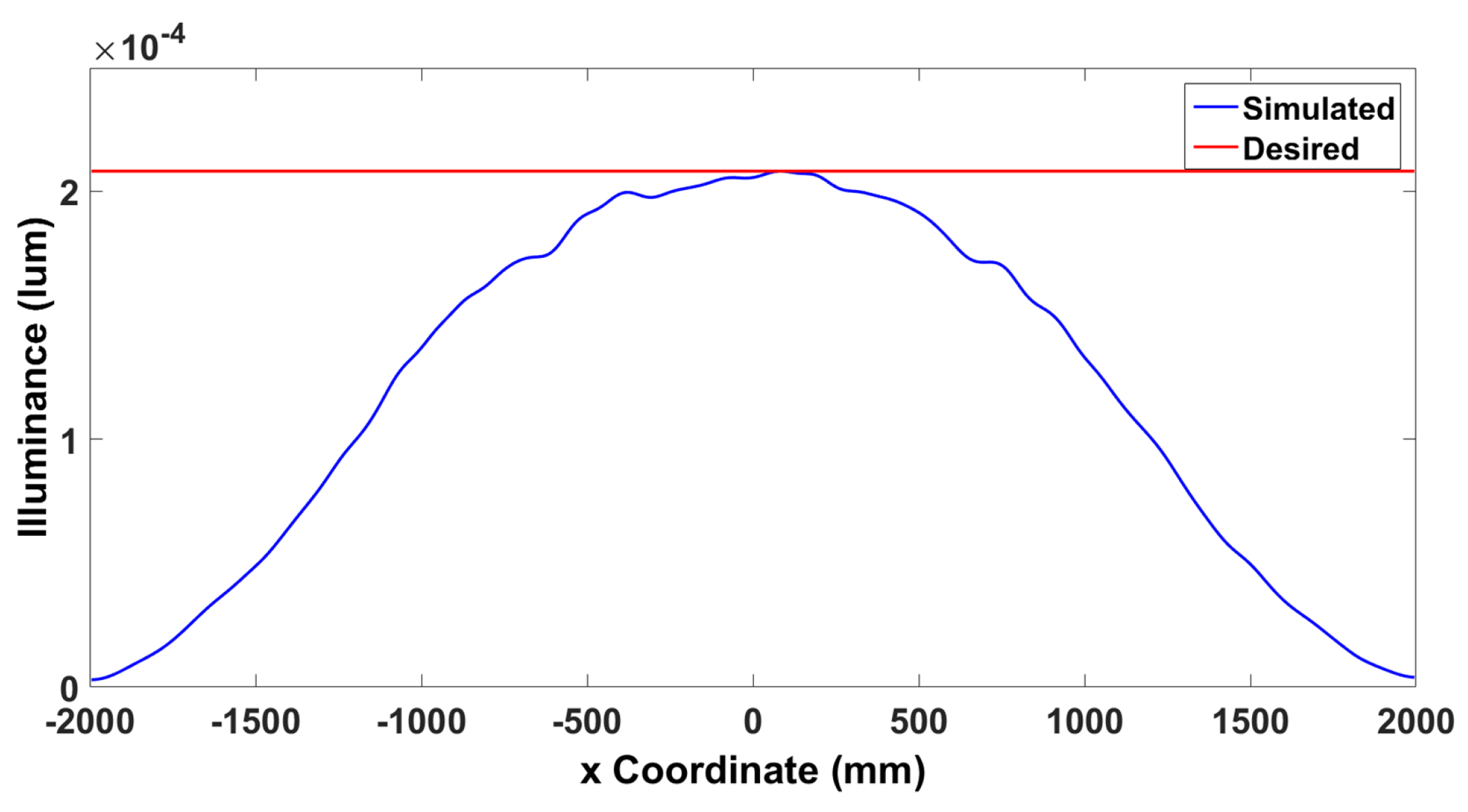
Figure 14 illustrates the distribution curve of the simulated illuminance S q as a function of position, along with that of the desired illuminance D q . The difference between a simulated and desired illuminance is a suitable metric for quantifying the quality of a candidate design solution.
The metric developed here to measure the quality of a candidate solution is given by the expression:
f L ( x ) = q = 1 k ( ( D q - S q ) + ( D q + 1 - S q + 1 ) ) · Δ q 2
where Δ q is the difference between the x-coordinates and q + 1 , where q { 1 , 2 , 3 , . . . , k } and where k is the number of discretized points on each illuminance curve.
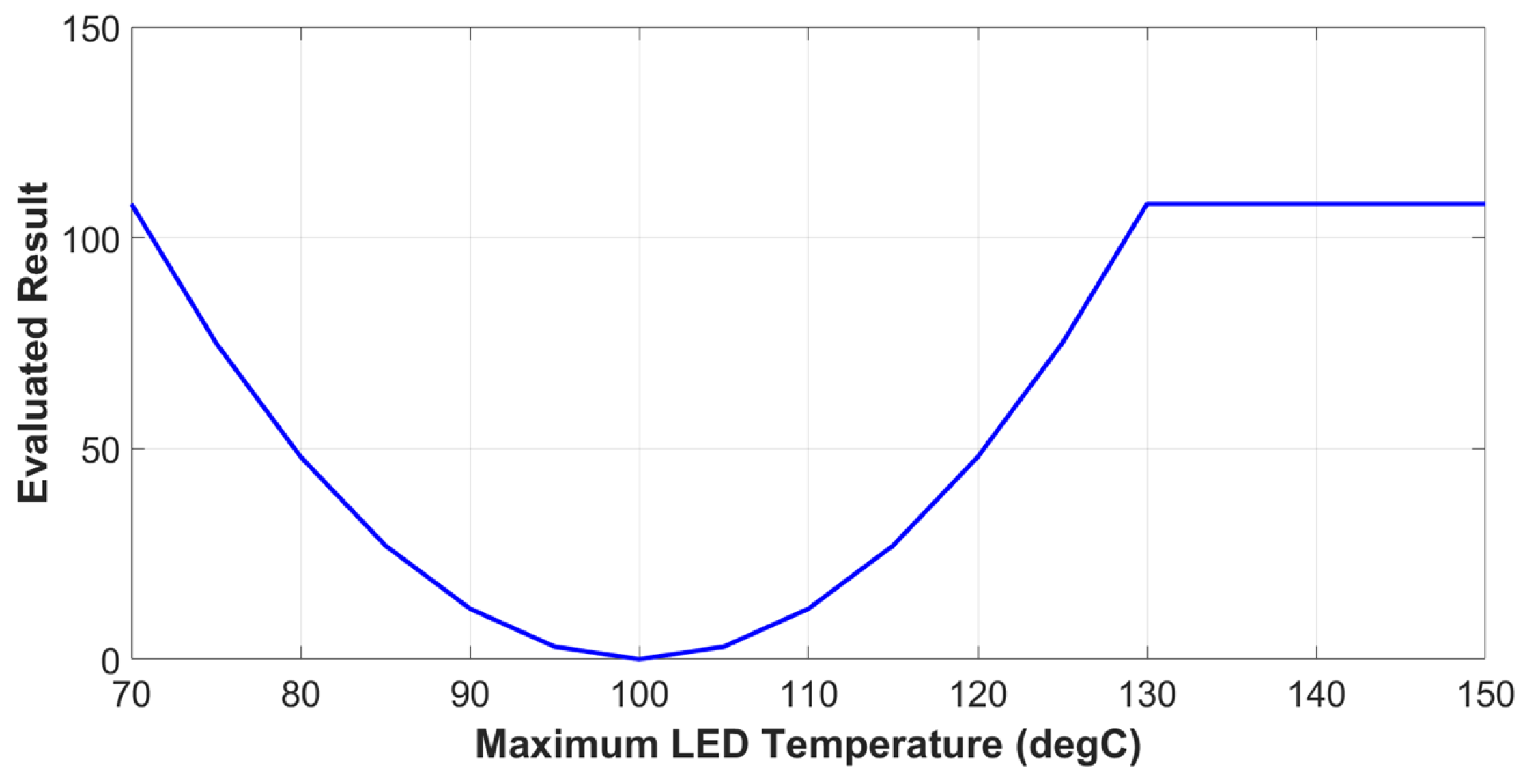
Next, heat dissipation is considered. The maximum temperature of all LED chips is evaluated directly by COMSOL, and the quality of a candidate solution is given by the expression:
f T ( x ) = 0 . 12 · T M A X 2 - 24 · T M A X + 1200 if T M A X 130   ° C 108 if T M A X > 130   ° C .
Expression (2) was empirically defined in such a way that the evaluation function values increase when the temperature values are far from 100 C. Figure 15 illustrates the expression (2), where the minimum of the function occurs when the temperature is 100 C. That is, a safety margin of 17% is allowed below the LED junction temperature of (120 C) (see Figure 2).
Both Expressions (1) and (2) are normalized from zero to one. Therefore, the overall cost function f ( x ) is a combination of f L ( x ) (lighting cost) and f T ( x ) (heat transfer cost):
f ( x ) = 0 . 3 · f T ( x ) + 0 . 7 · f L ( x )
where the scale factors 0.3 and 0.7 are chosen heuristically to give the desired balance between the two components of the cost.
The optimization algorithms in this research aim to find the best geometric parameters for the HP-LED luminaire. For each candidate solution, the optimization algorithm runs the first simulator to perform a thermal simulation and then runs the second simulator to perform a ray tracing analysis. The results of the simulations are combined as in (3). This process, when iterated, ultimately yields the optimized geometry of the HP-LED luminaire.
The optimization problem is summarized as follows:
min f ( x ) subject to : 2 m , n 6 50 W h , L h 200 2 H h 10 2 N f γ
where x Ω R p , Ω is the search space of the independent variables, p is the number of parameters to be optimized (in this case, p = 6 ) and m and n are the number of LEDs across the length and width of heat sink base, respectively. The heat sink parameters include W h , L h and H h , which are its width, length and thickness. N f is the number of fins in the heat sink base; that is, the independent variable of the optimization algorithm is x = [ m n W h L h H h N f ] . The γ value is dependent on L h :
γ = L h 16 + 0 . 75

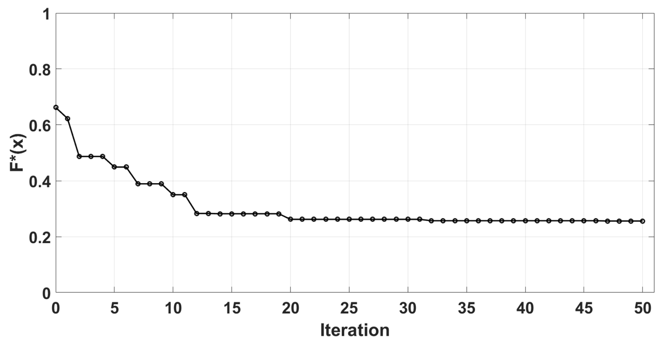
4.2. Deterministic Optimization Algorithms

Two deterministic algorithms are selected to optimize this multi-objective problem: quasi-Newton and Nelder–Mead. The quasi-Newton method is a derivative-based method that provides a balance between the simplicity of gradient descent and the speed of Newton’s method. The Nelder–Mead method is a direct search derivative-free method. The parameters used in the deterministic algorithms are shown in Table 6.
The independent variable values for both algorithms are initialized as shown in Table 7.

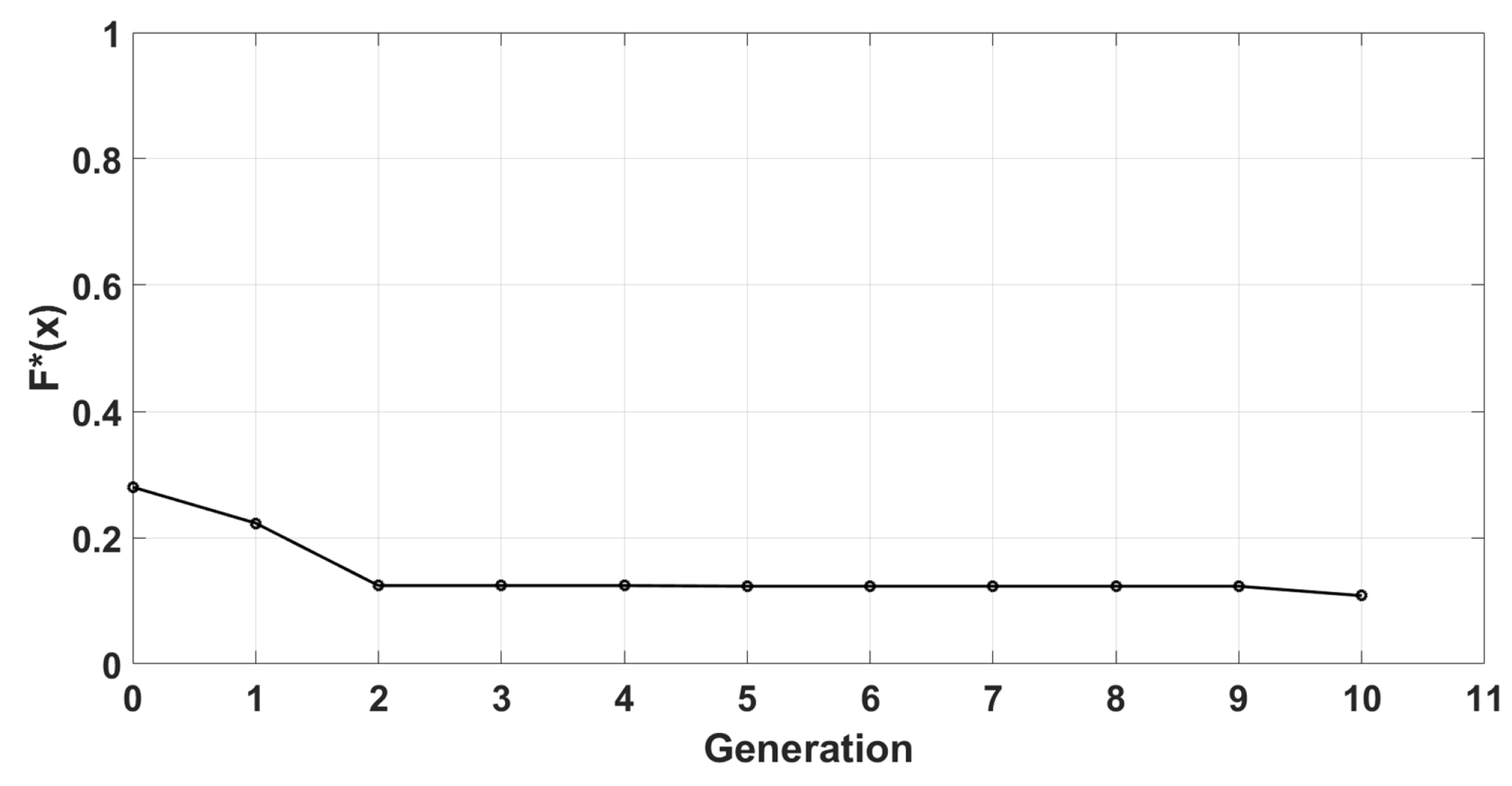
4.3. Evolutionary Algorithm

In this section, biogeography-based optimization (BBO) is used to design the luminaire. BBO is a stochastic, global optimization algorithm that has been applied to a wide variety of multidimensional, non-differentiable problems. It belongs to the evolutionary algorithm (EA) class and was motivated by species migration [34].
(a)
Initial population: the initial population of candidate solutions is generated randomly.
(b)
Population: the population size is constant (m).
(c)
Migration probability: immigration probability is the probability λ k that a given independent variable in the k-th candidate solution will be replaced. If an independent variable is replaced, then the emigrating candidate solution, which we suppose here is the j-th solution, is chosen with a probability that is proportional to its emigration probability μ j .
(d)
Elitism: the best individuals in each generation replace the worst individuals in the following generation. This method prevents the best individuals from being lost during a subsequent generation unless better individuals arise during the migration or mutation process.
(e)
Mutation: the value P m defines the mutation probability for each individual in each generation.
The parameters used in the BBO algorithm are shown in Table 8.

5. Results

5.1. Case Study I: Quasi-Newton Optimization

Initially, the quasi-Newton method is used to optimize f ( x ) . Figure 16 illustrates the evolution of the objective function value f ¯ ( x ) . The algorithm stopped after the 10th iteration because the step size was less than the step size tolerance. An objective function value f ¯ ( x ) = 0 . 149 was found, and the optimal parameter values are shown in Table 9. The LED temperature, which is defined as the maximum temperature of the LED chip (since the model is not detailed enough to calculate the LED junction temperature), reaches a maximum value of 104.6 C in the steady state, which is a feasible result for the LED junction temperature.

5.2. Case Study II: Nelder–Mead Optimization

Next, the Nelder–Mead method is used for optimization. Figure 17 illustrates the evolution of the objective function value f ¯ ( x ) . An objective function value f ¯ ( x ) = 0 . 256 was found, and the optimal parameter values are shown in Table 10. The LED temperature reaches a maximum value of 94.3 C in steady state, which is a feasible result for the LED junction temperature.

5.3. Case Study III: Biogeography-Based Optimization

The last optimization algorithm used is BBO [31]. Figure 18 illustrates the evolution of the objective function value f ¯ ( x ) . An objective function value f ¯ ( x ) = 0 . 108 was found, and the optimal parameter values are shown in Table 11. The LED temperature reaches a maximum value of 97.4 C in the steady state, which is a feasible result for the LED junction temperature. Figure 19 illustrates the illuminance distribution for the BBO-optimized solution of the HP-LED luminaire. Figure 20 illustrates the optimized HP-LED luminaire design. The computational time that was required to obtain the solution was 9 h on a PC with six CPUs and parallel programming.

6. Conclusions

The demand for electricity is growing at a faster rate than the capacity for electricity production. Energy efficiency in lighting not only narrows the gap between demand and production, but also includes other benefits, such as the reduction of CO 2 , which is emitted in the process of energy consumption and, thus, helps preserve the environment. HP-LEDs have emerged as an attractive and energy-efficient lighting alternative. Some of the technical challenges associated with HP-LEDs have been addressed in this paper.
Initial tests with HP-LEDs were restricted to a few low-dimensional heat sink designs and the LED array layout. At that early stage, optical accessories and cooling systems were not used to obtain a low-cost design. However, the results in this paper (summarized in Table 12) show that even with just a few parameters, it is possible to achieve satisfactory design results.
Case Studies I and II show that it is possible to design luminaires with six and eight HP-LEDs, keeping the LED temperature at about 100 C, but several difficulties are encountered when using deterministic algorithms for luminaire design optimization. For example, performance is highly dependent on the starting point. Therefore, a heuristic method (BBO) was used in this paper to achieve improved performance (Case Study III). Hybrid methods can achieve better results and should be implemented in the next step. Thus, the starting point of a deterministic algorithm could be the best individual found by the heuristic method.
It is possible with the proposed method to design HP-LED luminaires with a uniform lighting distribution, high luminous efficacy and low cost. The next step in this work is to implement new strategies to achieve even better results. For instance, a more uniform illumination could be obtained if the sources (LEDs) were fixed on a non-planar base (that is, a domed surface). This would entail the use of an additional heat sink geometry design parameter to adjust the tilt of each row of the LED array. Future research should also include other new parameters for the luminaire design, such as those related to auxiliary optics (lenses and reflection cones), to produce other desired illumination patterns on the target plane.
The threshold value of the luminaire size (that is, 200 mm × 200 mm) probably does not allow the use of the maximum number of LEDs in this paper (6 × 6) because of the maximum safe temperature of the LED chip. Future designs should therefore increase the maximum value of the luminaire size to 300 mm × 300 mm. Another observation is that the defined target plane of 16 m 2 (4 m × 4 m) may have been oversized for illumination by a single luminaire. Future research will reduce the target plane area to 9 m 2 (3 m × 3 m). Finally, future research should explore the use of other multi-objective optimization techniques and apply other variations of evolutionary algorithms in the search for better luminaire designs.

Acknowledgments

The authors acknowledge the CAPES (Coordination for the Improvement of Higher Education Personnel) Foundation, Ministry of Education of Brazil, for financial support through scholarship Proc. No BEX 2256/14-2 and Federal Institute of Goias for financial support of the research developed.

Author Contributions

These authors contributed equally to this work.

Conflicts of Interest

The authors declare no conflict of interest.

Nomenclature

A L E D LED chip area, m 2
Φ maximum luminous flux, lm
h heat transfer coefficient, W/(m 2 · K)
H f fins height, mm
H h heat sink height, mm
H E S M max max element size mesh of heat sink base object, mm
H E S M min min element size mesh of heat sink base object, mm
L E S M max max element size mesh of LED object, mm
L E S M min min element size mesh of LED object, mm
L h heat sink length, mm
L s MCPCB (metal core printed circuit board) length, mm
m number of LEDs in width
n number of LEDs in length
N f number of fins (each side)
P L E D LED power, W
T 0 initial temperature, C
W f fins width, mm
W h heat sink width, mm

References

  1. Navigant. Energy Savings Forecast of Solid-State Lighting in General Illumination Applications; Navigant Consulting, Inc.: Washington, DC, USA, 2014. [Google Scholar]
  2. Khan, T.Q.; Bodrogi, P.; Vinh, Q.T.; Winkler, H. (Eds.) LED Lighting: Technology and Perception; John Wiley & Sons: Weinheim, Germany, 2015. [Google Scholar]
  3. U.S. Department of Energy. Annual Energy Outlook 2015 with Projections to 2040; U.S. Department of Energy, Energy Information Administration: Washington, DC, USA, 2015.
  4. Uchida, Y.; Taguchi, T. Lighting theory and luminous characteristics of white light-emitting diodes. Opt. Eng. 2005, 44, 124003. [Google Scholar] [CrossRef]
  5. Navigant. Adoption of Light-Emitting Diodes in Common Lighting Applications: Snapshot of 2013 Trends; U.S. Department of Energy, Office of Energy Efficiency and Renewable Energy, Building Technologies Program: Washington, DC, USA, 2013.
  6. Khan, M.N. Understanding LED Illumination; CRC Press: Boca Raton, FL, USA, 2013. [Google Scholar]
  7. Jennic. Intelligent Street Lighting; Jennic Ltd.: Sheffield, UK, 2009. [Google Scholar]
  8. Gil, J.T.Q.M. Analise e Previsao da Evolucao do Custo da Electricidade em Portugal. Master’s Thesis, Universidade Tecnica de Lisboa, Lisboa, Portugal, 2010. (In Portuguese). [Google Scholar]
  9. Tichelen, P.V.; Geerken, T.; Jansen, B.; Vanden Bosch, M.; Van Hoof, V.; Vanhooydonck, L.; Vercalsteren, A. Final Report Lot 9: Public Street Lighting; VITO: Antwerp, Belgium, 2007. [Google Scholar]
  10. EPE-MME. Balanco Energetico Nacional-201; Empresa de Pesquisa Energetica, Ministerio de Minas e Energia: Rio de Janeiro, Brasil, 2011.
  11. Mottier, P. LED for Lighting Applications; John Wiley & Sons: Hoboken, NJ, USA, 2010; Volume 134. [Google Scholar]
  12. Evans, D.L. High luminance LEDs replace incandescent lamps in new applications. In Proceedings of theSPIE 3002, Light-Emitting Diodes: Research, Manufacturing, and Applications, San Jose, CA, USA, 4 April 1997; Volume 3002, pp. 142–153. [Google Scholar]
  13. Williams, B. A History of Light and Lighting, 2.2 ed. 1999. Available online: www.mts.net/william5/history/hol.htm (accessed on 11 October 2013).
  14. Barbosa, J.L.F.; Calixto, W.P.; Lima, R.A.; Alves, A.J.; Domingues, E.G. Thermal simulation and validation of 5W high power LED luminaire. In Proceedings of the IEEE 15th International Conference on Environment and Electrical Engineering, Rome, Italy, 10–13 June 2015; pp. 2216–2220. [Google Scholar]
  15. Jägerbrand, A.K. LED (Light-emitting diode) road lighting in practice: An evaluation of compliance with regulations and improvements for further energy savings. Energies 2016, 9, 5. [Google Scholar] [CrossRef]
  16. Lo, Y.-C.; Huang, K.-T.; Lee, X.-H.; Sun, C.-C. Optical design of a butterfly lens for a street light based on a double-cluster LED. Microelectron. Reliab. 2012, 52, 889–893. [Google Scholar] [CrossRef]
  17. Lenk, R.; Lenk, C. Practical Lighting Design with LEDs; Wiley-IEEE Press: Hoboken, NJ, USA, 2011. [Google Scholar]
  18. Jones, E.D. Light Emitting Diodes (LEDs) for General Illumination; OIDA-Optoelectronics Industry Development Association: Washington, DC, USA, 2001. [Google Scholar]
  19. Nuttall, D.R.; Shuttleworth, R.; Routledge, G. Design of a LED street lighting system. In Proceedings of the 4th IET International Conference on Power Electronics, Machines and Drives, New York, NY, USA, 2–4 April 2008; pp. 436–440. [Google Scholar]
  20. Bender, V.C.; Iaronka, O.; Marchesan, T.B. Study on the thermal performance of LED luminaire using finite element method. Proceedings of Industrial Electronics Society, IECON 2013-39th Annual Conference of the IEEE, Vienna, Austria, 10–13 November 2013; pp. 6099–6104. [Google Scholar]
  21. Ahn, B.L.; Park, J.-W.; Yoo, S.; Kim, J.; Leigh, S.-B.; Jang, C.-Y. Savings in cooling energy with a thermal management system for LED lighting in office buildings. Energies 2015, 8, 6658–6671. [Google Scholar] [CrossRef]
  22. Chang, M.-H.; Das, D.; Varde, P.V.; Pecht, M. Light emitting diodes reliability review. Microelectron. Reliab. 2012, 52, 762–782. [Google Scholar] [CrossRef]
  23. Mura, G.; Vanzi, M. Reliability prediction and real world for LED lamps. In Proceedings of the IEEE 21st International Symposium on the Physical and Failure Analysis of Integrated Circuits (IPFA), Singapore, 30 June–4 July 2014; pp. 207–210. [Google Scholar]
  24. Pryde, J.R. Methods of determining LED operating junction temperature experimental and theoretical. LED Prof. Rev. 2012, 32, 42–48. [Google Scholar]
  25. Luo, X.; Cheng, T.; Xiong, W.; Gan, Z.; Liu, S. Thermal analysis of an 80 W light-emitting diode street lamp. IET Optoelectron. 2007, 1, 191–196. [Google Scholar] [CrossRef]
  26. Luo, X.; Mao, Z.; Liu, S. Thermal design of a 16W LED bulb based on thermal analysis of a 4W LED bulb. In Proceedings of the 60th Electronic Components and Technology Conference (ECTC), IEEE, Las Vegas, NV, USA, 1–4 June 2010; pp. 1906–1911. [Google Scholar]
  27. Bai, K.; Wu, L.-G.; Nie, Q.-H.; Dai, S.-X.; Zhou, B.-Y.; Ma, X.-J.; Zheng, Z.-Y.; Zhang, F.-W. Thermal simulation and optimization of high-power white LED lamps. In Proceedings of the International Conference on Electronics, Communications and Control (ICECC), IEEE, Ningbo, China, 9–11 September 2011; pp. 573–576. [Google Scholar]
  28. Jakovenko, J.; Werkhoven, R.; Formánek, F.; Kunen, J.; Bolt, P.; Kulha, P. Thermal simulation and validation of 8W LED Lamp. In Proceedings of the 2011 12th International Conference on Thermal, Mechanical and Multi-Physics Simulation and Experiments in Microelectronics and Microsystems (EuroSimE), IEEE, Linz, Austria, 18–20 April 2011; pp. 1/4–4/4. [Google Scholar]
  29. Maaspuro, M.; Tuominen, A. Thermal analysis of LED spot lighting device operating in external natural or forced heat convection. Microelectron. Reliab. 2013, 53, 428–434. [Google Scholar] [CrossRef]
  30. Chi, W.H.; Chou, T.-L.; Han, C.-N.; Yang, S.-Y.; Chiang, K.-N. Analysis of thermal and luminous performance of MR-16 LED lighting module. IEEE Trans. Compon. Packag. Technol. 2010, 33, 713–721. [Google Scholar] [CrossRef]
  31. Barbosa, J.L.F.; Calixto, W.; Simon, D. High power LED luminaire design optimization. In Proceedings of the IEEE 16th International Conference on Environment and Electrical Engineering, Florence, Italy, 7–10 June 2016; pp. 1–6. [Google Scholar]
  32. COMSOL Multiphysics. Heat Transfer Module User’s Guide; COMSOL version 4.4; Comsol AB Group: Stockholm, Sweden, 2013.
  33. Barbosa, J.L.F. Secondary Lens Optimization Methodology for LED Lamps. Master’s Thesis, Federal University of Goias, Goiania, Brazil, 2013. (In Portuguese). [Google Scholar]
  34. Simon, D. Biogeography-based optimization. IEEE Trans. Evolut. Comput. 2008, 12, 702–713. [Google Scholar] [CrossRef]
Figure 1. Lighting market model.
Energies 10 00639 g001
Figure 2. Relationship between junction temperature and the lifetime of an HP-LED with maximum continuous forward current.
Energies 10 00639 g002
Figure 3. LED luminaire model and its parameters.
Energies 10 00639 g003
Figure 4. LED radiation patterns.
Energies 10 00639 g004
Figure 5. Ray tracing simulation.
Energies 10 00639 g005
Figure 6. Luminaire geometry model.
Energies 10 00639 g006
Figure 7. Photograph of the 5-W HP-LED luminaire.
Energies 10 00639 g007
Figure 8. HP-LED luminaire temperature measured by the thermocouple.
Energies 10 00639 g008
Figure 9. HP-LED luminaire temperature photo taken by the laser thermal camera.
Energies 10 00639 g009
Figure 10. LED model in the lighting simulator.
Energies 10 00639 g010
Figure 11. Experimental and simulated illuminance curves for a 5-W LED lamp without a lens [33].
Energies 10 00639 g011
Figure 12. Radiation pattern on a target plan of 2000 × 2000 (values in Lumens/mm 2 /ster).
Energies 10 00639 g012
Figure 13. Illuminance of the x-coordinate (cut line) on a target plane of 2000 × 2000 (values in Lumens/mm 2 ).
Energies 10 00639 g013
Figure 14. Distribution of illuminance; simulated (blue curve) and desired (red curve).
Energies 10 00639 g014
Figure 15. Temperature evaluation function.
Energies 10 00639 g015
Figure 16. Quasi-Newton evolution of the objective function value.
Energies 10 00639 g016
Figure 17. Nelder–Mead evolution of objective function value.
Energies 10 00639 g017
Figure 18. BBO evolution of the objective function value.
Energies 10 00639 g018
Figure 19. BBO optimized illuminance by the x-coordinate (cut line) on a target plane of 4 m × 4 m.
Energies 10 00639 g019
Figure 20. HP-LED luminaire for the optimized result.
Energies 10 00639 g020
Table 1. Material properties.
MaterialThermal Conductivity (W/(m 2 · K))
LED chip (GaN)130
Slug (Al)238
Outer plastic0.18
Plastic lens0.50
MCPCB201
Heat sink (Al)238
Table 2. Problem parameters.
SymbolValue
m>1
n>1
W h ≥50 mm
L h ≥50 mm
H h ≥2 mm
W f 2 mm
H f 20 mm
N f ≥2
L s 11.5 mm
A L E D 1.225 × 10 - 7 m 2
P L E D 5 W
h5 W/(m 2 · K)
T 0 27.2 C
H E S M max Wh/10 mm
H E S M min 0.18*HESM max mm
L E S M max 5 mm
L E S M min 0.4 mm
Table 3. Simulated high power (HP)-LED luminaire temperature values in the steady state.
Test PointDescriptionTemperature
P1LED 1111.7  C
P2LED 2111.7  C
P3LED 3111.7  C
P4LED 4111.7  C
P5heat sink76.7  C
P6heat sink76.6  C
P7heat sink76.6  C
P8heat sink76.7  C
Table 4. HP-LED luminaire temperature values in the steady state.
Test PointDescriptionThermal CameraTC
P1LED 1107.0  C-
P2LED 2104.5  C-
P3LED 3104.1  C-
P4LED 4100.0  C-
P5heat sink33.9  C-
P6heat sink33.5  C-
P7heat sink33.1  C-
P8heat sink75.2  C76.3  C
Table 5. Experimental and simulation results of LED temperature.
Test PointDescriptionSimulationExperimentError
P1LED 1111.7  C107.0  C4.4%
P2LED 2111.7  C104.5  C6.9%
P3LED 3111.7  C104.1  C7.6%
P4LED 4111.7  C100.0  C11.7%
P5, P6, P7, P8heat sink76.7  C76.3  C0.2%
Table 6. Parameters used in deterministic optimization algorithms.
ParameterValue
Number of independent variables6
Iteration limit50
Evaluation function target value 10 - 5
Table 7. Initial independent variable values for deterministic optimization algorithms.
mnWhLhHhNf
44150150510
Table 8. Parameters used in biogeography-based optimization (BBO).
ParameterValue
Number of independent variables6
Generation limit10
Objective function target value 10 - 5
Population size42
Table 9. Quasi-Newton optimized parameters.
mnWhLhHhNf
32194.158.1103
Table 10. Nelder–Mead optimized parameters.
mnWhLhHhNf
42192.1157.9510
Table 11. BBO optimized parameters.
mnWhLhHhNf
22160.093.0103
Table 12. Results.
Table 12. Results.
Algorithm f ¯ ( x ) mnWhLhHhNf
Quasi-Newton0.14932194.158.1103
Nelder-Mead0.25642192.1157.9510
BBO0.10822160.093.0103

