
Multi-Objective History Matching with a Proxy Model for the Characterization of Production Performances at the Shale Gas Reservoir


Abstract
:1. Introduction
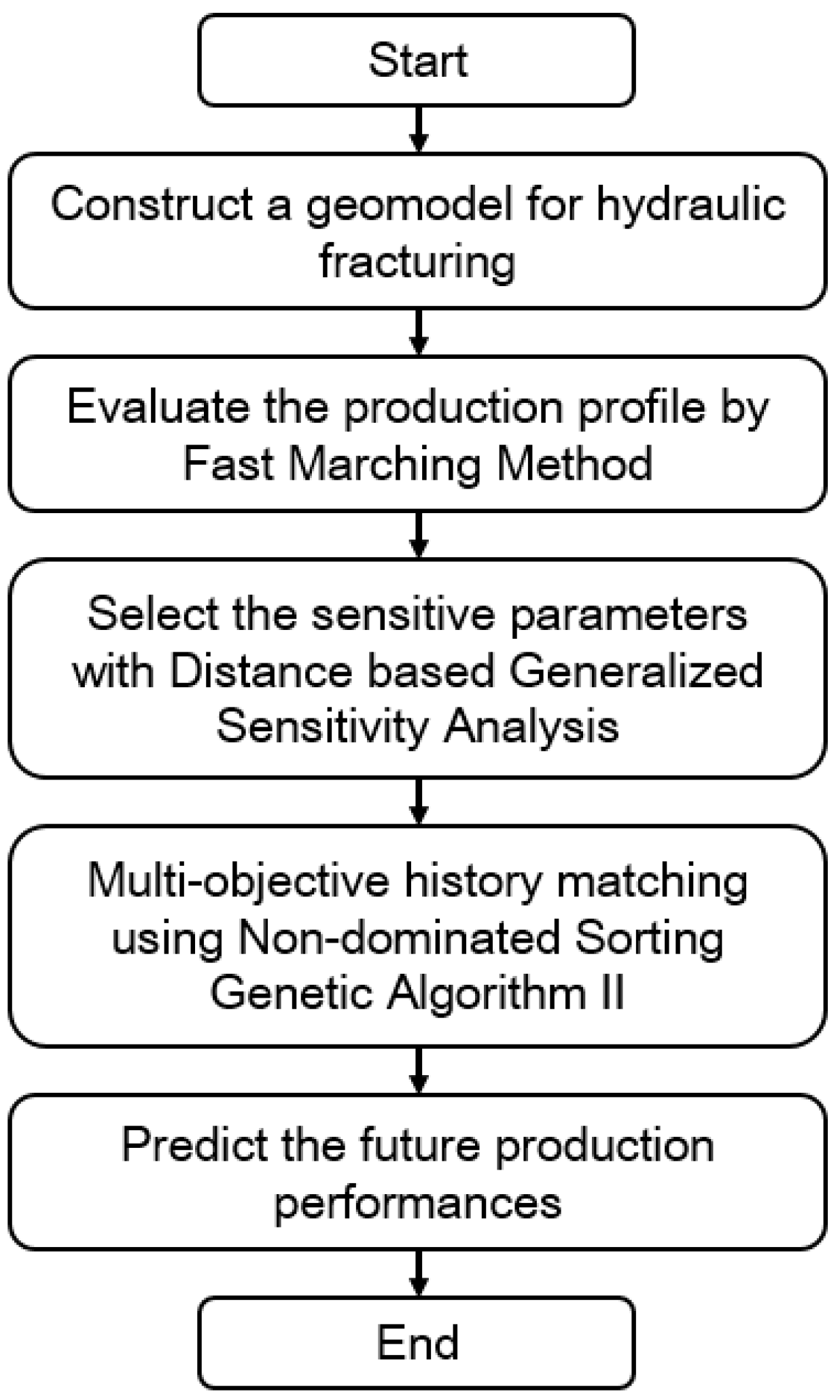
2. Methodology
2.1. FMM for the Proxy Modeling
2.2. DGSA for the Determination of the Effective Parameters
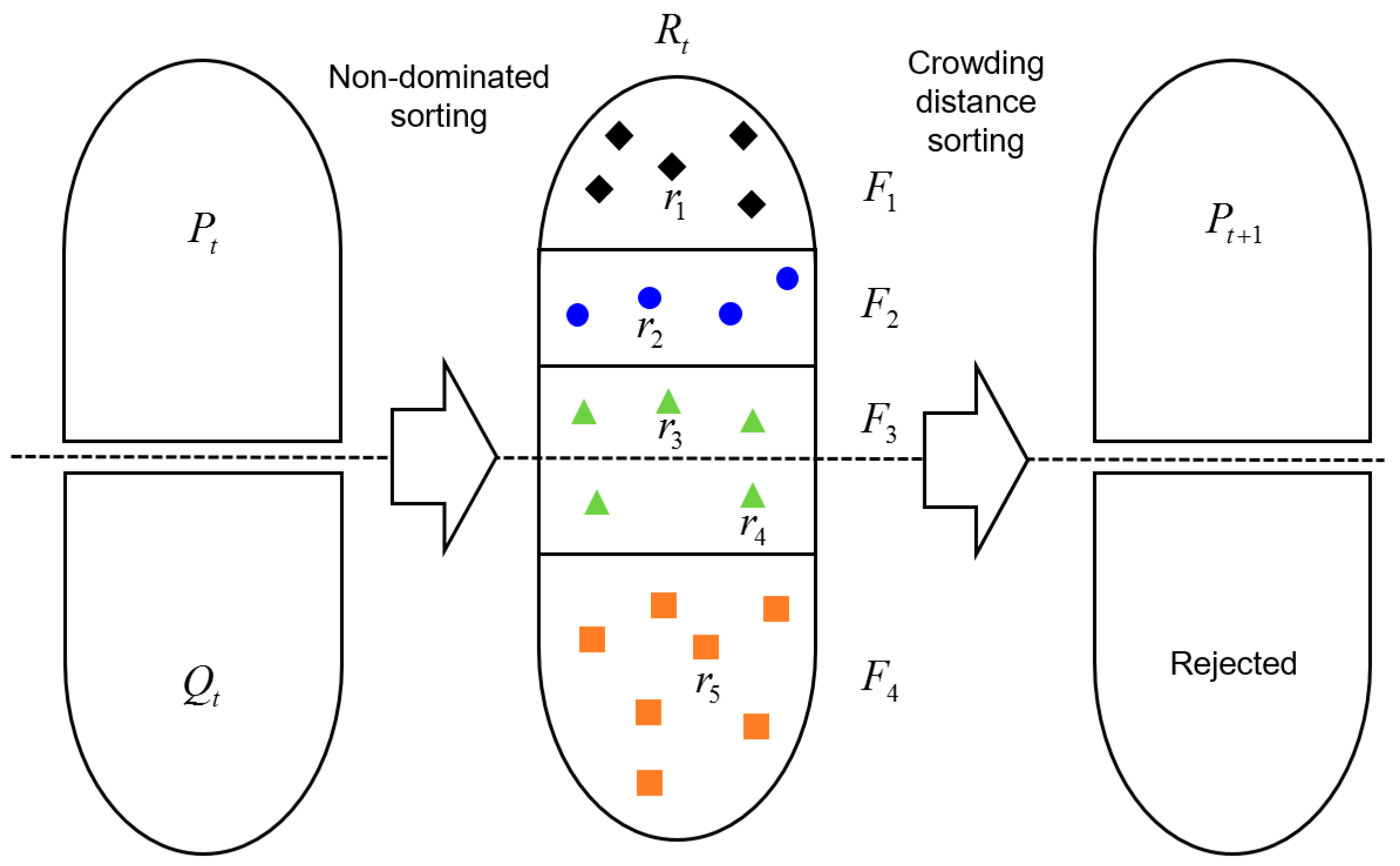
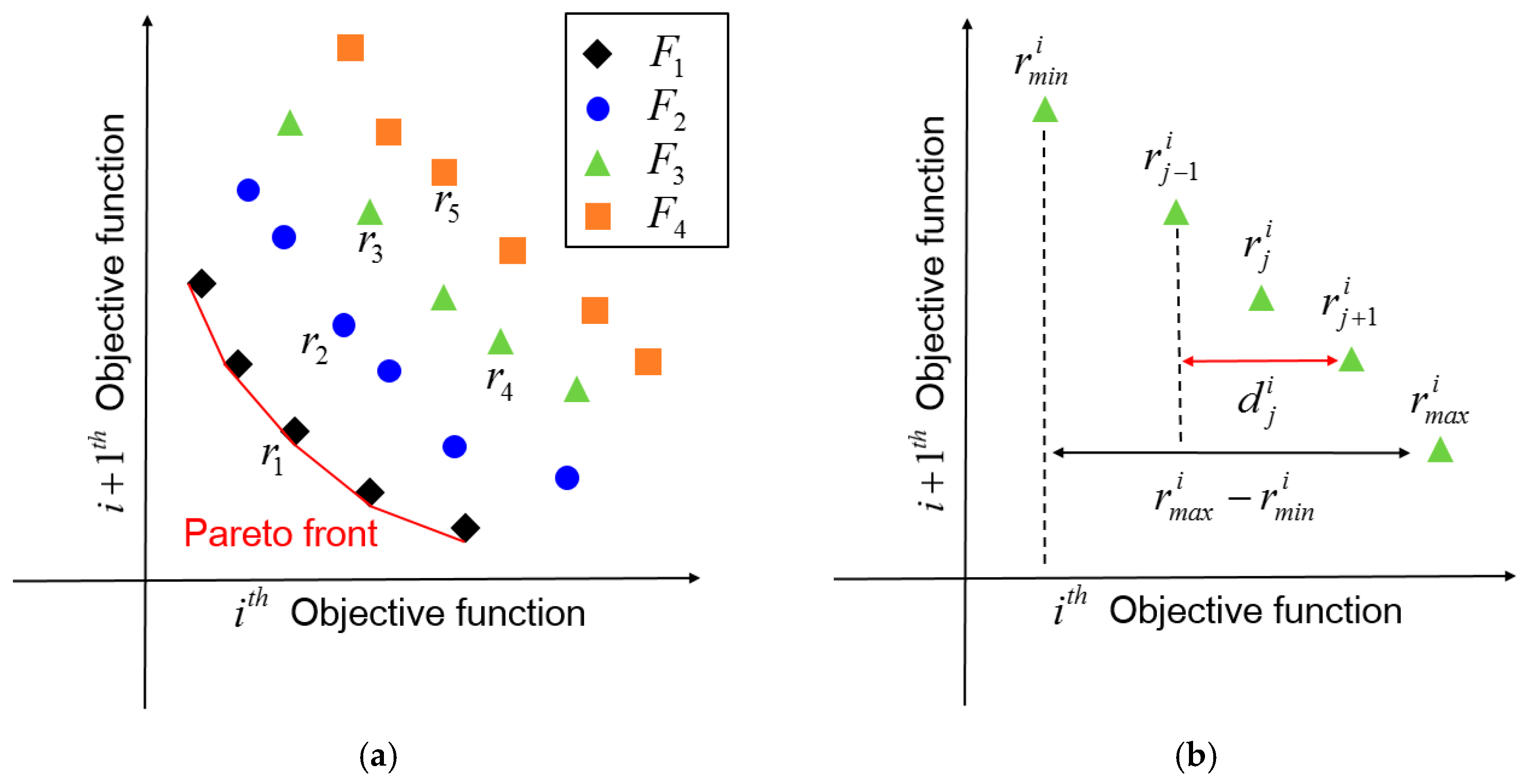
2.3. NSGA-II for the Multi-Objective Evolutionary Algorithm
3. Results and Discussion
3.1. Performance Test for the Validation of the FMM-Based Proxy Modeling
3.1.1. Description of a Synthetic Reservoir and the Testing Method
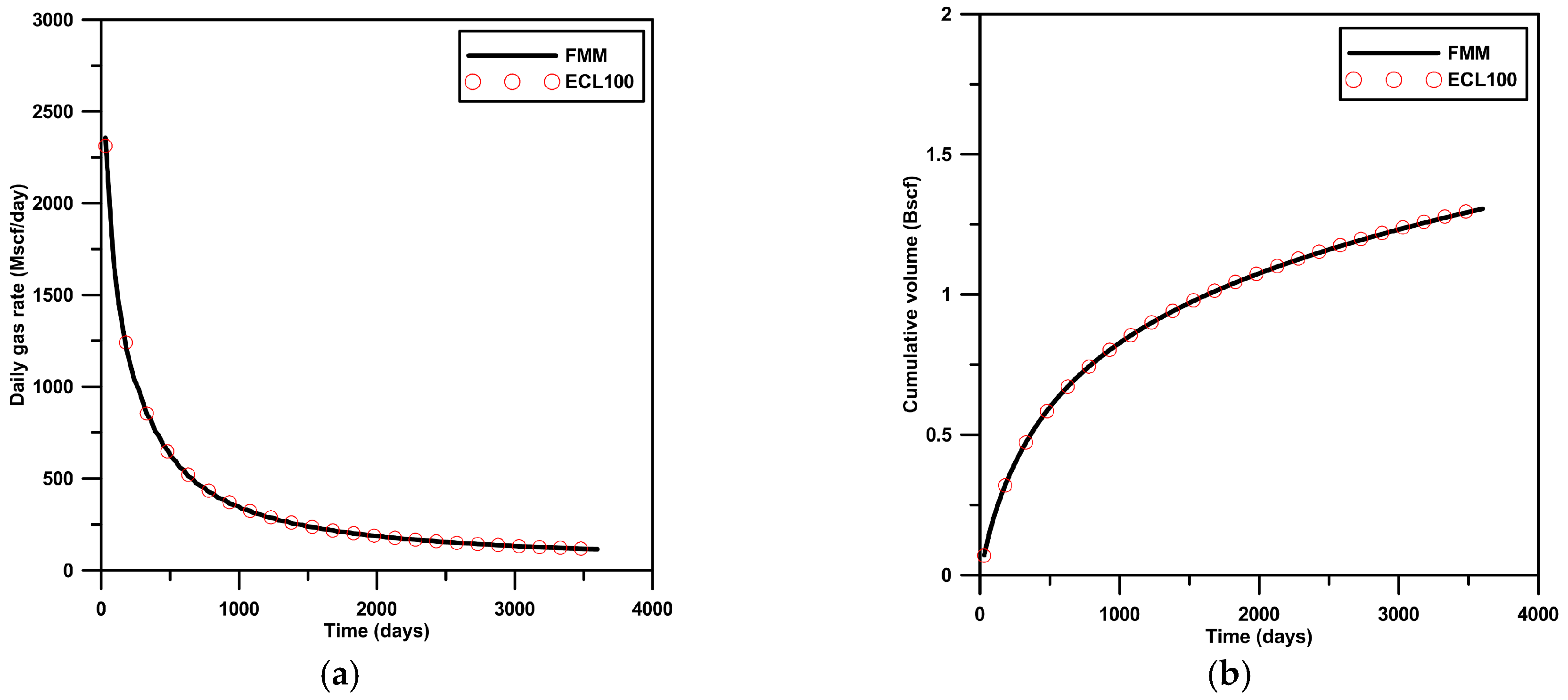
3.1.2. Results of the FMM-Based Proxy Modeling
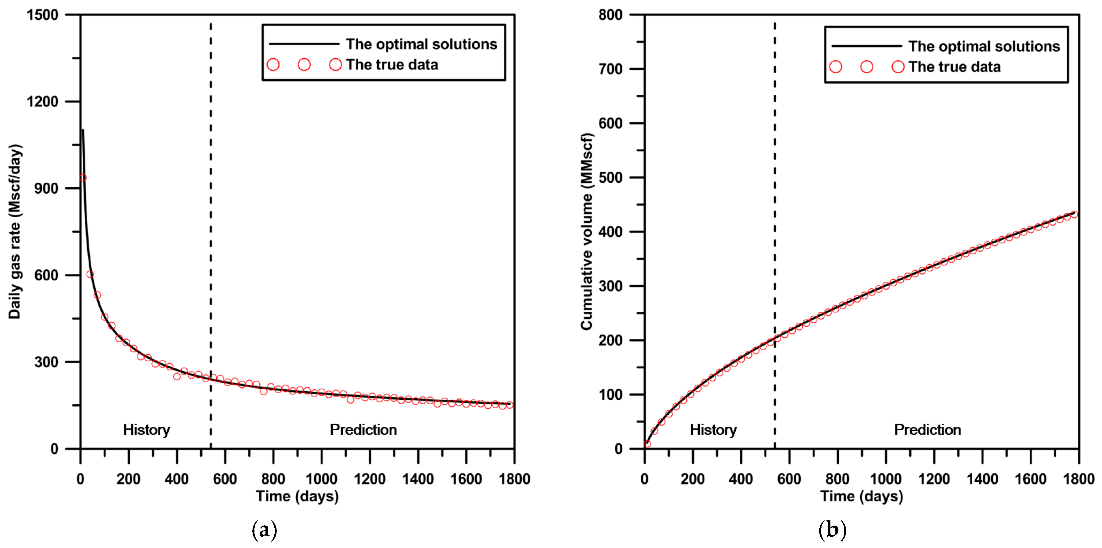
3.2. Application: Multi-Objective History Matching with FMM-Based Proxy Modeling
3.2.1. Description of the Gas-Production Data and Assumptions
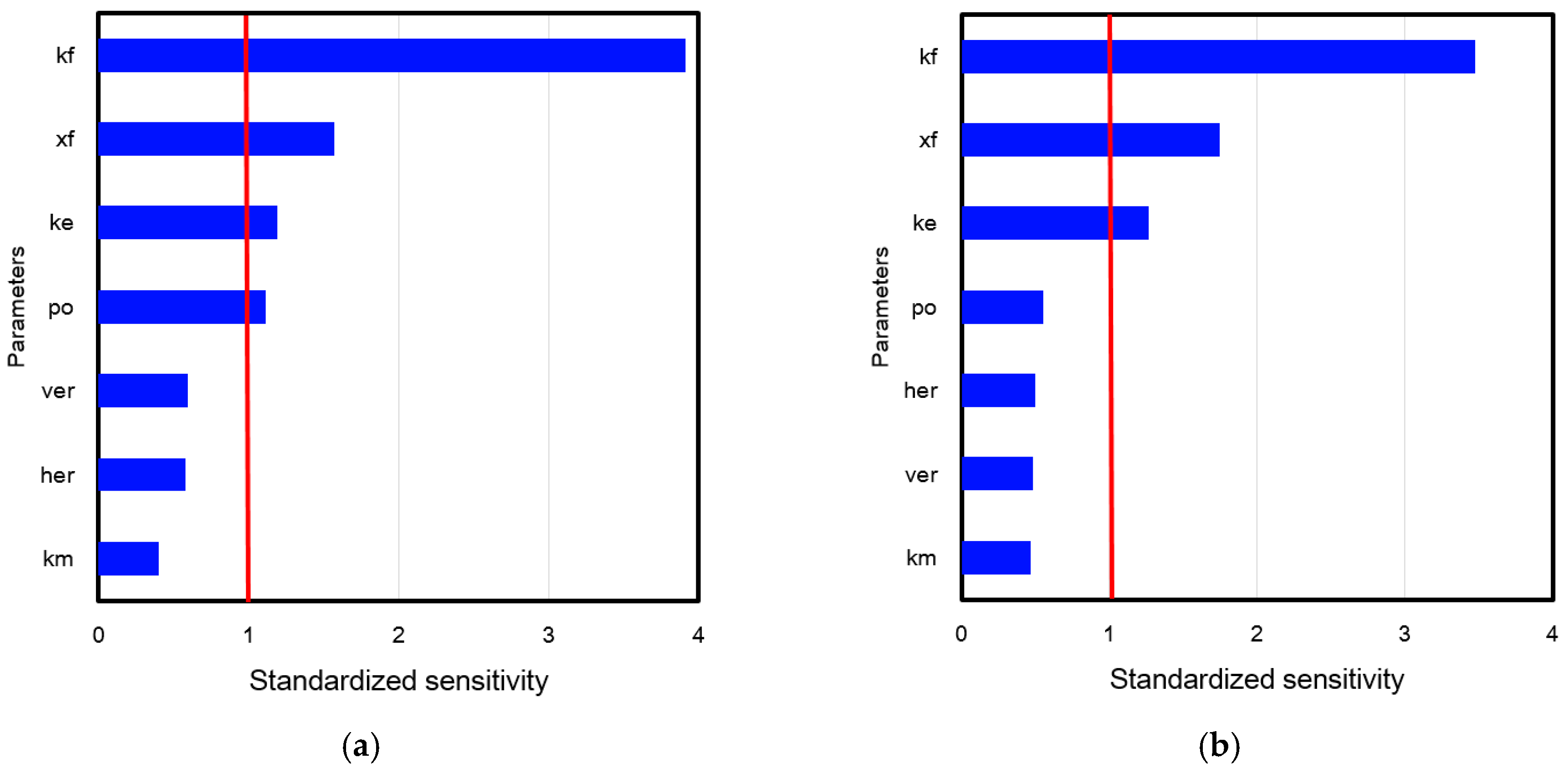
3.2.2. Sensitivity Analysis Based on the DGSA
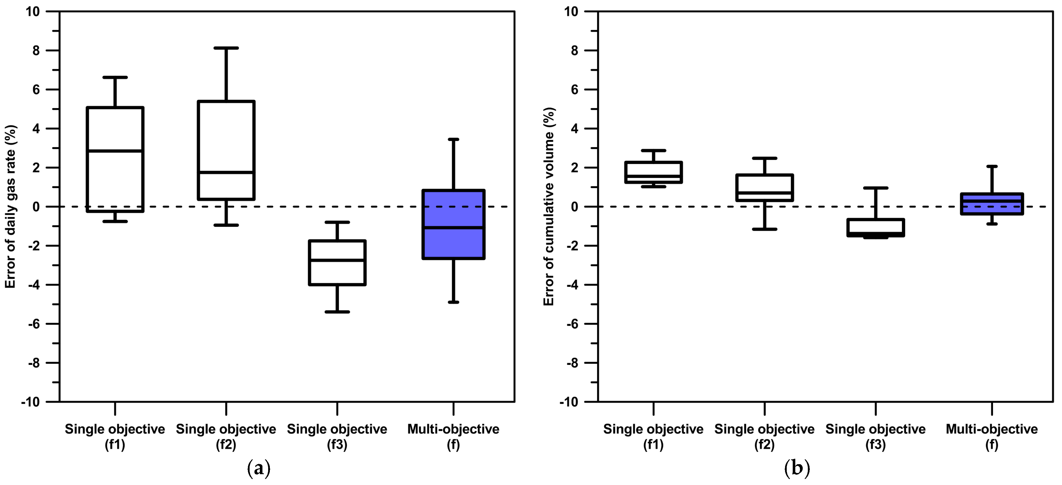
3.2.3. Multi-Objective History Matching
4. Conclusions
Acknowledgement
Author Contributions
Conflicts of Interest
References
- Anderson, D.M.; Liang, P.; Okouma, V. Probabilistic forecasting of unconventional resources using rate transient analysis: Case studies. In Proceedings of the SPE Americas Unconventional Resources Conference, Pittsburgh, PA, USA, 5–7 June 2012. SPE 155737-MS. [Google Scholar]
- German, G.M.; Navarro-Rosales, R.A.; Dubost, F.X. Production forecasting for shale gas exploration prospects based on statistical analysis and reservoir simulation. In Proceedings of the SPE Latin America and Caribbean Petroleum Engineering Conference, Mexico City, Mexico, 16–18 April 2012. SPE 152639-MS. [Google Scholar]
- Batycky, R.P.; Blunt, M.J.; Thiele, M.R. A 3D field-scale streamline-based reservoir simulator. SPE Reserv. Eng. 1997, 12, 246–254. [Google Scholar] [CrossRef]
- Jin, J.; Lim, J.; Lee, H.; Choe, J. Metric space mapping of oil sands reservoirs using streamline simulation. Geosyst. Eng. 2011, 14, 109–113. [Google Scholar] [CrossRef]
- Kulkarni, K.N.; Datta-Gupta, A.; Vasco, D.W. A streamline approach for integrating transient pressure data into high resolution reservoir models. In Proceedings of the SPE European Petroleum Conference, Paris, France, 24–25 October 2000. SPE-65120-MS. [Google Scholar]
- Saputelli, L.; Malki, H.; Canelon, J.; Nikolaou, M.A. Critical overview of artificial neural network applications in the context of continuous oil field optimization. In Proceedings of the SPE Annual Technical Conference and Exhibition, San Antonio, TX, USA, 29 September–2 October 2002. SPE-77703-MS. [Google Scholar]
- Min, B.; Park, C.; Kang, J.M.; Park, H.; Jang, I.S. Optimal well placement based on artificial neural Network incorporating the productivity potential. Energy Source Part A 2011, 33, 1726–1738. [Google Scholar] [CrossRef]
- Kim, K.; Ju, S.; Ahn, J.; Shin, H.; Shin, C.; Choe, J. Determination of key parameters and hydraulic fracture design for shale gas productions. In Proceedings of the Twenty-fifth International Ocean and Polar Engineering Conference, Kona, HI, USA, 21–26 June 2015. ISOPE-I-15-812. [Google Scholar]
- Sethian, J.A.; Vladimirsky, A. Fast methods for the eikonal and related hamilton–jacobi equations on unstructured meshes. Proc. Natl. Acad. Sci. USA 2000, 97, 5699–5703. [Google Scholar] [CrossRef] [PubMed]
- Li, C.; King, M.J. Integration of pressure transient data into reservoir models using the Fast Marching Method. In Proceedings of the SPE Europec featured at 78th EAGE Conference and Exhibition, Vienna, Austria, 30 May–2 June 2016. SPE 180148-MS. [Google Scholar]
- Zhang, Y.; Bansal, N.; Fujita, Y.; Datta-Gupta, A.; King, M.J.; Sankaran, S. From streamlines to fast marching: Rapid simulation and performance assessment of shale gas reservoirs using diffusive time of flight as a spatial coordinate. SPE J. 2016, 21, 1883–1898. [Google Scholar] [CrossRef]
- Xie, J.; Yang, C.; Gupta, N.; King, M.; Datta-Gupta, A. Depth of investigation and depletion in unconventional reservoirs with fast-marching methods. SPE J. 2015, 20, 831–841. [Google Scholar] [CrossRef]
- Kim, J.; Kang, J.M.; Park, Y.; Lim, S.; Park, C.; Park, J. Probabilistic estimation of shale gas reserves implementing Fast Marching Method and monte carlo simulation. In Proceedings of the ASME 2016 35th International Conference on Ocean, Offshore and Arctic Engineering, Busan, Korea, 19–24 June 2016. OMAE2016-54167. [Google Scholar]
- Min, B.; Kang, J.M.; Chung, S.; Park, C.; Jang, I. Pareto-based multi-objective history matching with respect to individual production performance in a heterogeneous reservoir. J. Petrol. Sci. Eng. 2014, 122, 551–566. [Google Scholar] [CrossRef]
- Velez-Langs, O. Genetic algorithms in oil industry: An overview. J. Petrol. Sci. Eng. 2005, 47, 15–22. [Google Scholar] [CrossRef]
- Ballester, P.J.; Carter, J.N. A parallel real-coded genetic algorithm for history matching and its application to a real petroleum reservoir. J. Petrol. Sci. Eng. 2007, 59, 157–168. [Google Scholar] [CrossRef]
- Lee, K.; Jeong, H.; Jung, S.; Choe, J. Characterization of channelized reservoir using ensemble Kalman filter with clustered covariance. Energy Explor. Exploit. 2013, 31, 17–29. [Google Scholar] [CrossRef]
- Lee, J.; Jeong, H.; Jung, S.; Choe, J. Improvement of ensemble smoother with clustered covariance for channelized reservoirs. Energy Explor. Exploit. 2013, 31, 713–726. [Google Scholar] [CrossRef]
- Xie, J.; Yang, C.; Gupta, N.; King, M.J.; Datta-Gupta, A. Integration of shale-gas-production data and microseismic for fracture and reservoir properties with the Fast Marching Method. SPE J. 2015, 20, 347–359. [Google Scholar] [CrossRef]
- Leem, J.; Lee, K.; Kang, J.M.; Park, Y.; Park, J. History matching with ensemble Kalman filter using Fast Marching Method in shale gas reservoir. In Proceedings of the SPE/IATMI Asia Pacific Oil & Gas Conference and Exhibition, Nusa Dua, Bali, Indonesia, 20–22 October 2015. SPE 176164-MS. [Google Scholar]
- Han, Y.; Park, C.; Kang, J.M. Prediction of nonlinear production performance in waterflooding project using a multi-objective evolutionary algorithm. Energy Explor. Exploit. 2011, 29, 129–142. [Google Scholar] [CrossRef]
- Deb, K.; Pratap, A.; Agarwal, S.; Meyarivan, T. A fast and elitist multiobjective genetic algorithm: NSGA-II. IEEE Trans. Evol. Comput. 2002, 6, 182–197. [Google Scholar] [CrossRef]
- Min, B.; Park, C.; Jang, I.; Lee, H.; Chung, S.; Kang, J.M. Multi-objective history matching allowing for scale-difference and the interwell complication. In Proceedings of the 75th EAGE Conference & Exhibition Incorporating SPE EUROPEC 2013, London, UK, 10–13 June 2013. [Google Scholar]
- Min, B.; Park, C.; Jang, I.; Kang, J.M.; Chung, S. Development of pareto-based evolutionary model integrated with dynamic goal programming and successive linear objective reduction. Appl. Soft Comput. 2015, 35, 75–112. [Google Scholar] [CrossRef]
- Min, B.; Kang, J.M.; Lee, H.; Jo, S.; Park, C.; Jang, I. Development of a robust multi-objective history matching for reliable well-based production forecasts. Energy Explor. Exploit. 2016, 34, 795–809. [Google Scholar] [CrossRef]
- Park, H.Y.; Datta-Gupta, A.; King, M.J. Handling conflicting multiple objectives using pareto-based evolutionary algorithm during history matching of reservoir performance. J. Petrol. Sci. Eng. 2015, 125, 48–66. [Google Scholar] [CrossRef]
- Min, B.; Nwachukwu, A.; Srinivasan, S.; Wheeler, M.F. Selection of geologic models based on pareto-optimality using surface deformation and CO2 injection data for the in Salah gas sequestration project. In Proceedings of the SPE Annual Technical Conference and Exhibition, Dubai, UAE, 26–28 September 2016. SPE 181569-MS. [Google Scholar]
- Fenwick, D.; Scheidt, C.; Caers, J. Quantifying asymmetric parameter interactions in sensitivity analysis: Application to reservoir modeling. Math. Geosci. 2014, 46, 493–511. [Google Scholar] [CrossRef]
- Pappenberger, F.; Beven, K.J.; Ratto, M.; Matgen, P. Multi-method global sensitivity analysis of flood inundation models. Adv. Water Resour. 2008, 31, 1–14. [Google Scholar] [CrossRef]
- Bastidas, L.A.; Gupta, H.V.; Sorooshian, S.; Shuttleworth, W.J.; Yang, Z.L. Sensitivity analysis of a land surface scheme using multicriteria methods. J. Geophys. Res. Atmos. 1999, 104, 19481–19490. [Google Scholar] [CrossRef]
- Srinivas, N.; Deb, K. Multiobjective optimization using nondominated sorting in genetic algorithms. Evol. Comput. 1994, 2, 221–248. [Google Scholar] [CrossRef]
- Dong, Z.; Holditch, S.A.; McVay, D.A.; Ayers, W.B.; Lee, W.J.; Morales, E. Probabilistic assessment of world recoverable shale gas resources. SPE Econ. Manag. 2015, 7, 72–82. [Google Scholar] [CrossRef]


| Input Parameters (Unit) | Fixed Value | Uncertain Value † |
|---|---|---|
| Reservoir size (x, y, z) (m) | (1200, 600, 165) | – |
| Grid size (Δx, Δy, Δz) (m) | (3, 3, 3) | – |
| Fracture half-length (m) | 120, 90, 135, 120, 105 (from the left-hand side in Figure 6) | – |
| Fracture permeability (millidarcy, md) | 10 | – |
| Gas viscosity (cp) | 0.015 | – |
| Gas saturation (fraction) | 0.66 | – |
| Gas formation volume factor (rm3/sm3) | 0.012 | – |
| Initial reservoir pressure (MPa) | 34.47 | – |
| Well-flowing pressure (MPa) | 6.89 | – |
| Reservoir temperature (°C) | 104.44 | – |
| Total compressibility (1/kPa) | 0.00003 | – |
| Porosity (fraction) | – | Triangular (0.06, 0.08, 0.10) |
| Matrix permeability (md) | – | Triangular (0.0001, 0.0007, 0.0013) |
| Enhanced permeability in the stimulated reservoir volume (md) | – | Triangular (0.005, 0.007, 0.009) |
| Input Parameters (Unit) | Fixed Value | Uncertain Value |
|---|---|---|
| Reservoir size (x, y, z) (m) | (375, 300, 135) | – |
| Grid size (Δx, Δy, Δz) (m) | (3, 3, 3) | – |
| Gas viscosity (cp) | 0.02 | – |
| Gas saturation (fraction) | 0.6 | – |
| Gas formation volume factor (rm3/sm3) | 0.012 | – |
| Initial reservoir pressure (MPa) | 10.34 | – |
| Well flowing pressure (MPa) | 3.44 | – |
| Reservoir temperature (°C) | 37.7 | – |
| Total compressibility (1/kPa) | 0.00003 | – |
| Porosity (fraction) | 0.005–0.08 | |
| Matrix permeability (md) | 0.0001–0.0003 | |
| Enhanced permeability in the stimulated reservoir volume (md) | – | 0.0005–0.005 |
| Fracture permeability (md) | – | 0.01–0.1 |
| Fracture half-length (m) | – | 15–60 |
| Horizontal enhanced ratio † | – | 0.2–0.4 |
| Vertical enhanced ratio ‡ | – | 0.8–1.6 |
| Objective Function | During the History-Matching Period | During the Prediction Period | Error of EUR (%) | ||
|---|---|---|---|---|---|
| Error of Daily Gas Rate (%) | Error of Cumulative Volume (%) | Error of Daily Gas Rate (%) | Error of Cumulative Volume (%) | ||
| 1.75 | 2.12 | 4.83 | 1.83 | 2.87 | |
| 2.58 | 1.04 | 4.94 | 1.15 | 2.48 | |
| 3.00 | 1.88 | 2.34 | 1.40 | 1.35 | |
| (mean value) | 2.08 | 2.34 | 2.42 | 0.45 | 0.43 |
© 2017 by the authors. Licensee MDPI, Basel, Switzerland. This article is an open access article distributed under the terms and conditions of the Creative Commons Attribution (CC BY) license (http://creativecommons.org/licenses/by/4.0/).
Share and Cite
Kim, J.; Kang, J.M.; Park, C.; Park, Y.; Park, J.; Lim, S. Multi-Objective History Matching with a Proxy Model for the Characterization of Production Performances at the Shale Gas Reservoir. Energies 2017, 10, 579. https://doi.org/10.3390/en10040579
Kim J, Kang JM, Park C, Park Y, Park J, Lim S. Multi-Objective History Matching with a Proxy Model for the Characterization of Production Performances at the Shale Gas Reservoir. Energies. 2017; 10(4):579. https://doi.org/10.3390/en10040579
Chicago/Turabian StyleKim, Jaejun, Joe M. Kang, Changhyup Park, Yongjun Park, Jihye Park, and Seojin Lim. 2017. "Multi-Objective History Matching with a Proxy Model for the Characterization of Production Performances at the Shale Gas Reservoir" Energies 10, no. 4: 579. https://doi.org/10.3390/en10040579
APA StyleKim, J., Kang, J. M., Park, C., Park, Y., Park, J., & Lim, S. (2017). Multi-Objective History Matching with a Proxy Model for the Characterization of Production Performances at the Shale Gas Reservoir. Energies, 10(4), 579. https://doi.org/10.3390/en10040579