Load Signature Formulation for Non-Intrusive Load Monitoring Based on Current Measurements

Abstract

In this paper we present a new methodology for the formulation of efficient load signatures towards the implementation of a near-real time Non-Intrusive Load Monitoring (NILM) approach. The purpose of this work relies on defining representative current values regarding the 1st, 3rd and 5th harmonic orders to be utilized in the load signatures formulation. A measurement setup has been developed and steady-state measurements have been performed in a Low Voltage residence. A data processing methodology is proposed aiming to depict representative current values for each harmonic order in order to keep the load signature short and simple. In addition, a simple disaggregation scheme is proposed under linear equations for the disaggregation mode in order to examine the near-real time application of the methodology. The analysis indicates that the developed load signatures could be efficient for a per second application rate of the NILM algorithm. The results show that the higher harmonic currents facilitate the identification performance. Finally, the analysis concludes that for combinations that include appliances with intense harmonic content, the phase angle of the higher for harmonic currents should also be considered to the load signatures formulation.

1. Introduction

The Smart Grid Concept (SGC) relies basically on advanced metering capabilities regarding the real or near real time recording of the grid’s operational characteristics, and on upgraded automation concerning immediate switching operations [1,2]. The Smart Home paradigm is expected to constitute the core of the SGC in Low Voltage (LV) networks and is likely to be implemented via the installation of Smart Meters with upgraded metering features, and advanced data acquisition and analysis tools. Smart Meters are expected to provide detailed measurements of the energy consumption of each residence in order to promote Demand Side Management (DSM) actions towards energy efficiency strategic plans [3]. Moreover, in order to facilitate consumers to understand their consumption behavior and to analyze its dependency on specific consumption patterns, further functional capabilities are investigated to be embedded in Smart Meters. These capabilities refer to Load Identification (LI) functions that aim to provide information about the identity of the turned-on appliance, its working duration, and its consumption [4]. Such information is highly appreciated by both the consumers and the aggregator (e.g., Distribution Network Operator) since it could support (a) the consumers to understand their consumption behavior and possibly alter it in order to reduce their electricity cost, and (b) the aggregator to launch DSM programs that provide incentives towards energy efficiency, peak shaving, peak shifting and more.

LI is based on the notion that the consumption/working behavior of each appliance could be described under a unique and distinct formulation, which embeds information about all features related to the appliance’s operational/electrical attributes. This formulation is commonly known as Load Signature (LS). In practice, LS constitutes a suitably configured data structure that describes concisely the behavior of the load during its operation. The early attempts for LI involved either installing sensors on every appliance or an intermediate monitoring system that recorded its operation [5]. Generally, this Intrusive Load Monitoring (ILM) method is inconvenient due to its high cost for large scale implementations. A simpler methodology, namely the Non-Intrusive Load Monitoring (NILM), was proposed in the early 1990s [6]. The advantage of NILM is that it requires only one power meter for the monitoring and identification of the plugged appliances, installed at the main feeding panel. The challenge, though, in NILM methodologies lies on the LI efficiency, since the recorded and measured signal is actually an aggregated one that embeds the information from all simultaneously working appliances. The efficient disaggregation of this signal into its components depends greatly on the formulation of unique and distinct LSs. In case of simultaneous operation of two or more appliances, LI involves finding an appropriate combination of the individual LSs of the active appliances. Therefore, the higher the uniqueness of these load signatures the easier the identification procedure.

Many NILM methodologies have been proposed to deal with the development of both efficient LSs and LI approaches. The overall efficiency of a NILM algorithm is heavily dependent on the complexity and size of the LS, which in turn depends on the selection of the appliances’ features [7,8,9,10,11]. Most of the published methodologies utilize features like the active and reactive power, current and voltage harmonics, transient behavior particularly during the activation, current waveform characteristics, and techniques based on V-I trajectory [12,13,14,15,16]. For example in [17] the analysis utilizes the transient response time and transient energy on the power signatures. These features are obtained via a discrete wavelet transform as it has been considered more suitable than the short-time Fourier transform. In all aforementioned methodologies the selected features are utilized either individually or combined, in order to enhance the efficiency of the LSs.

One crucial aspect regarding the utilization of harmonics in NILM methodologies relies on how this information should be depicted and embedded in LSs. For example in [18] it has been found that the odd harmonic currents constitute efficient features for the load signature formulation. Thus, the question raised in this case refers to the highest order of odd harmonic currents to be utilized. Naturally, the more the harmonic currents depicted, the higher the uniqueness of the LS. On the other hand, a high complexity regarding the LS formulation could cause unacceptable computation burden for the disaggregation mode of the NILM algorithm. In this latter case, the identification accuracy could worsen at the expense of the algorithm’s implementation time. In [19] a NILM scheme is employed to identify special loads of a microgrid. Several Fast Fourier Transform (FFT) spectrum components are considered for the formulation of the LSs, while sub-harmonics and interharmonics are also examined due to the nature of the examined loads. The work in [20] presents a thorough survey about NILM methodologies, analyzing four load types. Type-I refers to appliances with only two states of operation (on/off). Type-II loads are multi-state appliances with a finite number of operational states and repeatable switching pattern. Type-III includes appliances with variable power draw characteristics, but without fixed number of operational states. Finally, Type-IV involves appliances that remain active throughout weeks or days consuming energy at a constant rate. The analysis in [20] concludes that NILM methods under steady-state that utilize harmonic current have a relatively low accuracy for Type-III loads and for overlapping features for consumer electronics of Type-I and Type-II category. The consideration of harmonic currents has been proven to contribute in formulating more distinct LSs [21,22,23], but it has not been fully clarified how these harmonic features could be efficiently disaggregated in NILM algorithms under simultaneous operation of various appliances.

In [24] an approach of multi point sensing and group control in NILM techniques is presented. The technique used the first 8 harmonic of the current signature for the classification with neural network classifier and Bayes classifier demonstrating a recognition accuracy of up to 99.18%. Although high identification accuracy is performed, the proposed technique depends on large data since 8 harmonic orders are utilized. In [25] a low cost NILM approach is proposed. The basic utilized data for the LS formulation concern the peak current values. The performance of this approach is significantly decreased when more than three appliances are operating simultaneously. In [26] the LSs are formulated based on harmonic currents up to the 15th order. Moreover, the phase of each order is also measured and the total rms current is also utilized. These aforementioned data have been acquired under a high sampling frequency via an expensive measurement device. Finally, in [27] an interesting approach is presented. The methodology utilizes a Data Acquisition (DAQ) card to measure rms current values and as stated by the authors, an unknown appliance can be identified according to the following metrics: (a) Similarity of magnitude arrays of the consumed current level, (b) Similarity of standard distribution array of the consumed current level and (c) Operation time and duration of each appliance type.

In this paper, we examine the contribution of the Odd-Order Harmonic Currents (OOHC) towards the enhancement of LSs that are formed only by the amplitude of the currents at the fundamental frequency (i.e., 50 Hz) and at 3rd and 5th harmonic orders (i.e., 150 Hz and 250 Hz respectively) for each appliance. For this investigation, we have obtained measurements from a different mix of appliances inside a residence with a single phase installation. Each appliance was measured under stand-alone operation in order to develop the LS database of the residence. These measurements concern the instantaneous current at the main feeding panel of the residence. Then the measured current is processed (FFT application) and the amplitudes of the 1st, 3rd and 5th harmonic orders are calculated. Based on these latter values the load signatures and the load identification (disaggregation scheme is performed). In addition, we have realized scenarios regarding the simultaneous operation of appliance combinations, in order to examine whether the efficient decomposition of aggregated signals is possible for successful LI. The main aim of this analysis is to highlight the contribution of the OOHC to the development of more distinct LSs especially for nonlinear LV loads and, in turn, to facilitate the recognition of these appliances. Moreover, this work intends to examine if LSs consisting only of harmonic current amplitudes up to the 5th order can be used to reliably decompose an aggregated signal. In such case, we assess the performance of the identification procedure by determining the magnitude of the recognition error.

The rest of the paper is organized as follows: Section 2 provides all information about the measurement setup and the performed measurements. Moreover, the proposed methodology for the LS formulation is explained and the LSs for the test case in this work are presented. In Section 3 a NILM approach for near-real time load identification is analyzed and various scenarios regarding simultaneous operation of appliances to be identified are presented. Recommendations and suggestions for further improvements are commented. Finally, Section 4 is devoted to conclusions.

2. Measurements and Load Signature Formulation

In this section the measurement setup is analyzed and all relevant information about the performed measurements are provided. Moreover, the proposed methodology about the LS formulation is explained and the formed LS database is presented.

2.1. Measurement Setup

The measurement setup consists of a common AC current probe (LEM PR630, measuring range ±60 A with accuracy ±1%, DC to 20 kHz frequency range) and a voltage optoisolated transducer (measuring range ±600 V). The outputs of the voltage transducer and current probe (transfer coefficients 5 V/600 V and 10 mV/A, respectively) were acquired using a data acquisition card (DAQ card, NI PXI-6123). Sampling rate was set at 50,000 samples/s. Voltage and current waveforms captured by the DAQ card contained 50,000 samples each corresponding to an acquisition period of 1 s or 50 periods of the fundamental frequency of the power line. Current acquisition was configured to be in synchronization to the voltage waveform.

Acquired analog current waveform was processed and further FFT (Fast Fourier Transform) analyzed in real time by means of an application developed in LabVIEW graphical programming language. FFT analysis revealed the amplitudes and frequencies of current fundamental and harmonic components (current power spectrum). The frequency interval df of the power spectrum resulted from FFT analysis, i.e., the minimum frequency difference between successive harmonic components of the signal, is given by df = r/n, where, r is the sampling rate (50,000 samples/s) and n is the number of samples contained in each analyzed waveform (5000 samples). Taking into account the above acquisition parameters, the frequency interval of the current power spectrum, presented in this work, is 1 Hz. The recording frequency of the measured data was set to 1 Hz (1 sample/s).

Low-pass filter is intrinsic to the Fast Fourier Transform (FFT) algorithm to comply with Nyquist’s theorem. As a sampling rate of 50 kSamples/s was used for the acquisition of current in this work, a low-pass filter with a cut-off frequency set at 25 kHz was applied to acquired waveforms (Nyquist theorem). The FFT analysis applied to the filtered current signal in the frequency range dc—25 kHz revealed a power spectrum consisting of a normal array of peaks at fundamental (50 Hz) and higher harmonics (150 Hz, 250 Hz, …) with diminishing amplitudes as frequency increases with no intermediate peaks and an almost negligible white noise amplitude. A measure of the white noise contribution to the variation of the observed harmonics amplitude is given by the measured standard deviation of the peak amplitudes and its interpretation and handling lies within the subjects of this work.

2.2. Measured Appliances

All measurements have been carried out in a residence with a single-phase installation, using various appliances. The installed nominal capacity of the residence is 25 kVA. The measurements involved (a) the stand-alone operation of each appliance so as to capture its own and unique operational characteristics for the development of its LS, and (b) various scenarios with simultaneous operation of appliance combinations. The recorded data were the amplitudes of the currents at 50 Hz, 150 Hz and 250 Hz, i.e., the fundamental current, 3rd and 5th harmonic currents respectively. Prior to any measurement, we measured the background in order to identify the harmonic content at the main feeding panel. This has been found to be in the order of 10⁻² regarding both the 3rd and 5th order harmonic currents.

The first aim of this work is to investigate whether specific harmonic current amplitudes (fundamental, 3rd and 5th) can formulate efficient LSs. This will result in less computation effort for the data processing and the identification procedure, and lower cost for the measurement setup. The second aim is to examine the potential for real time matching of aggregated individual LSs with the input signal for load identification.

Table 1. Measured appliances and appliance combinations for the examined residence.

Measured Appliances
PC	Hair-dryer (hot)	Coffee-maker	Vacuum	Electric iron
TV	Resistive-heater	Toaster	Refrigerator	Blender
Measured Appliance Combinations
1	Hair-dryer (hot)	Vacuum	Resistive-heater
2	Coffee-maker	Electric iron	Resistive-heater	Toaster
3	Coffee-maker	Toaster	Refrigerator	Blender
4	PC	Electric iron	TV	Resistive-heater

lists the examined appliances along with the appliance combinations measured for this residence. It is clarified that each appliance has been measured individually in order to form its LS and the load combinations have been measured in order to test the efficiency of the disaggregation scheme in this work.

One of the greatest challenges in NILM methodologies is to ensure that the LSs would be robust and distinct under the simplest possible formulation and the fewest possible operational features of the appliances. Obviously, if the LS of an appliance consist of many operational and electrical characteristics it would be distinct enough. However, such a choice yields complex LSs with large databases and increased computational burden. Another difficulty concerns appliances with various operational states/modes for which most of the utilized operational features in their LSs follow these alterations. Naturally, these alterations and/or variations would be present under the operation of load combinations and could affect the identification performance. Therefore, in such cases the question raised concerns the capability for the consideration of these variations in the LSs. In this work such an attempt is investigated under the consideration of discrete values that could be representative for the different operational modes and will be explained in detail in the next section. Figure 1a–c and Figure 2a–c show the recorded current amplitudes at 50 Hz, 150 Hz and 250 Hz for the laptop and the vacuum appliances.

The results for the laptop measurements constitute a representative example regarding appliances with varied operational modes. The appliance has been recorded for 5 min (i.e., 300 values under a recording frequency of 1 sample/s). The laptop is a typical load with varied consumption due to the screen’s and processor’s adjustments to the user’s preferences. It is highly possible to capture additional variations under a higher recording frequency. One first observation is that all graphs share an identical pattern, which means that amplitude harmonics vary similarly at each operating mode. The most interesting observation, though, is that there are two operational modes with different current amplitude values and significant variation range. There are two concerns in this case: Firstly, a decision should be made about which of these operational modes should be utilized for the formulation of the laptop’s LS. Secondly, the identification of this appliance can be hindered, as other appliances may fall within the variation range between the two operation modes. Finally, it should be stated that smoother variations during each operational state should also be considered during the LS formulation.

In Figure 2a–c the recorded current values for the vacuum appliance are presented for the 3 examined frequencies. In this case one operational mode exists that is relatively constant with very smooth variations. Thus, the LS could be formed based on few values for each frequency that would be representative for the whole steady state operation period.

2.3. Load Signatures Formulation

In the present work the formulation of the LSs relies on the utilization of the OOHCs and specifically on the 1st, 3rd and 5th order harmonic currents. This facilitates the identification both of non-linear loads within an aggregated signal, and of appliances with similar consumption. Therefore, the proposed LS formulation is as follows:

$${\mathrm{LS}}_i=\left[\left[I_{50i}^a\right],\left[I_{150i}^b\right],\left[I_{250i}^c\right]\right]$$

(1)

where:

• LS_i is the load signature of appliance i;
• indices 50, 150 and 250 represent the fundamental nominal current, the 3rd and the 5th harmonic currents respectively;
• indices $a\in N^{*}$ and $b,c\in N$ with $a\ge 1$ and $b,c\ge 0$ denote the number of values utilized for the respective part of the LS.

Indices a, b and c express the number of representative current values that have been utilized for each harmonic order (1st, 3rd and 5th) in order to form the load signature of each appliance. These representative values are supposed to be efficient for load recognition under aggregated measured current values. For example, in Figure 3 the recorded values of the fundamental current for the PC (desktop) appliance are presented in descending order. The values in Figure 3 refer to a typical operation of the appliance for approximately 5 min.

Based on the data presented in Figure 3 the variation range of the fundamental current for this appliance is [0.86–1.3] A. The following questions are raised in this case:

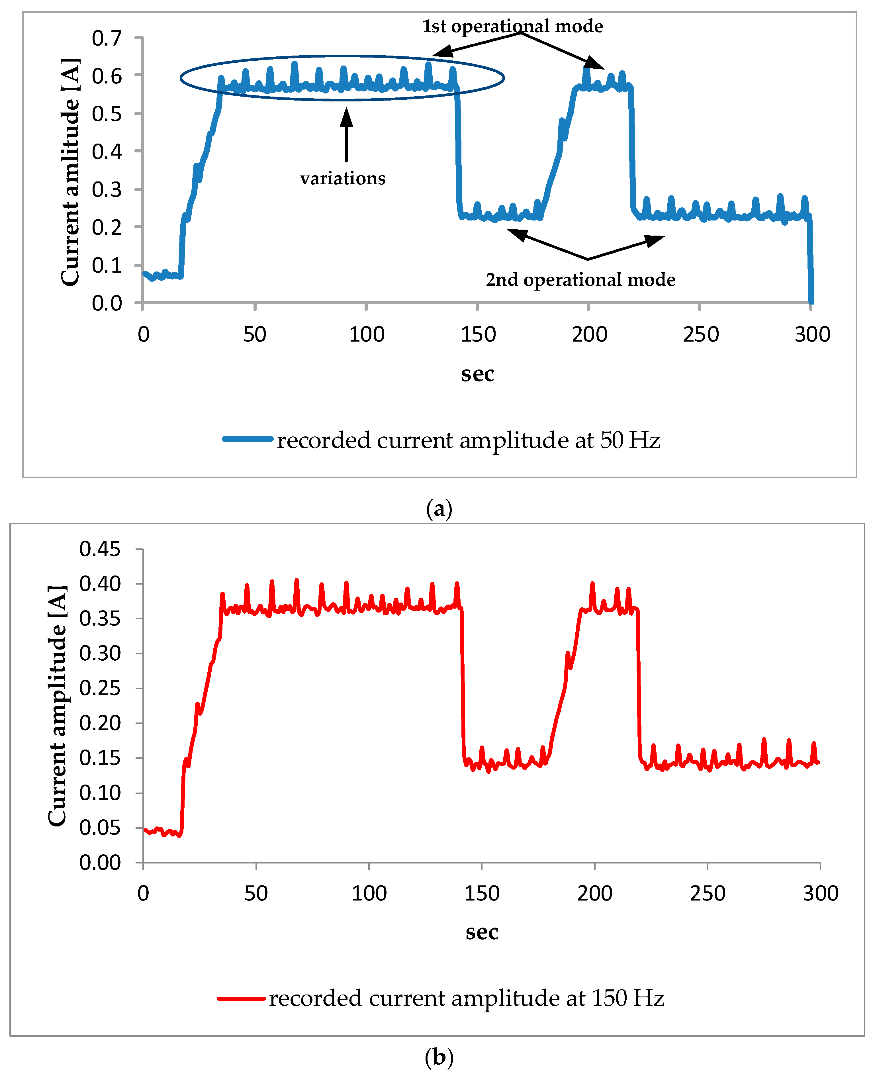
• Which one of these values should be considered for the formulation of the first part of the LS in (1) since all of them describe the operation of this appliance under steady-state? A simple and quick approach could be the mean value. The problem here is that the higher the variation range, the less representative the mean value would be. This could greatly hinder the performance of a NILM algorithm and the identification accuracy of the appliance.
• If the consideration of a single value yields inefficient LS, then how many values should be utilized in order to ensure that the operation of the appliance is captured in most of the possible operational modes? Τhe answer in this question defines the number of a, b and c indices of the LS.

In order to answer these questions the following methodology is proposed for the formulation of each LS:

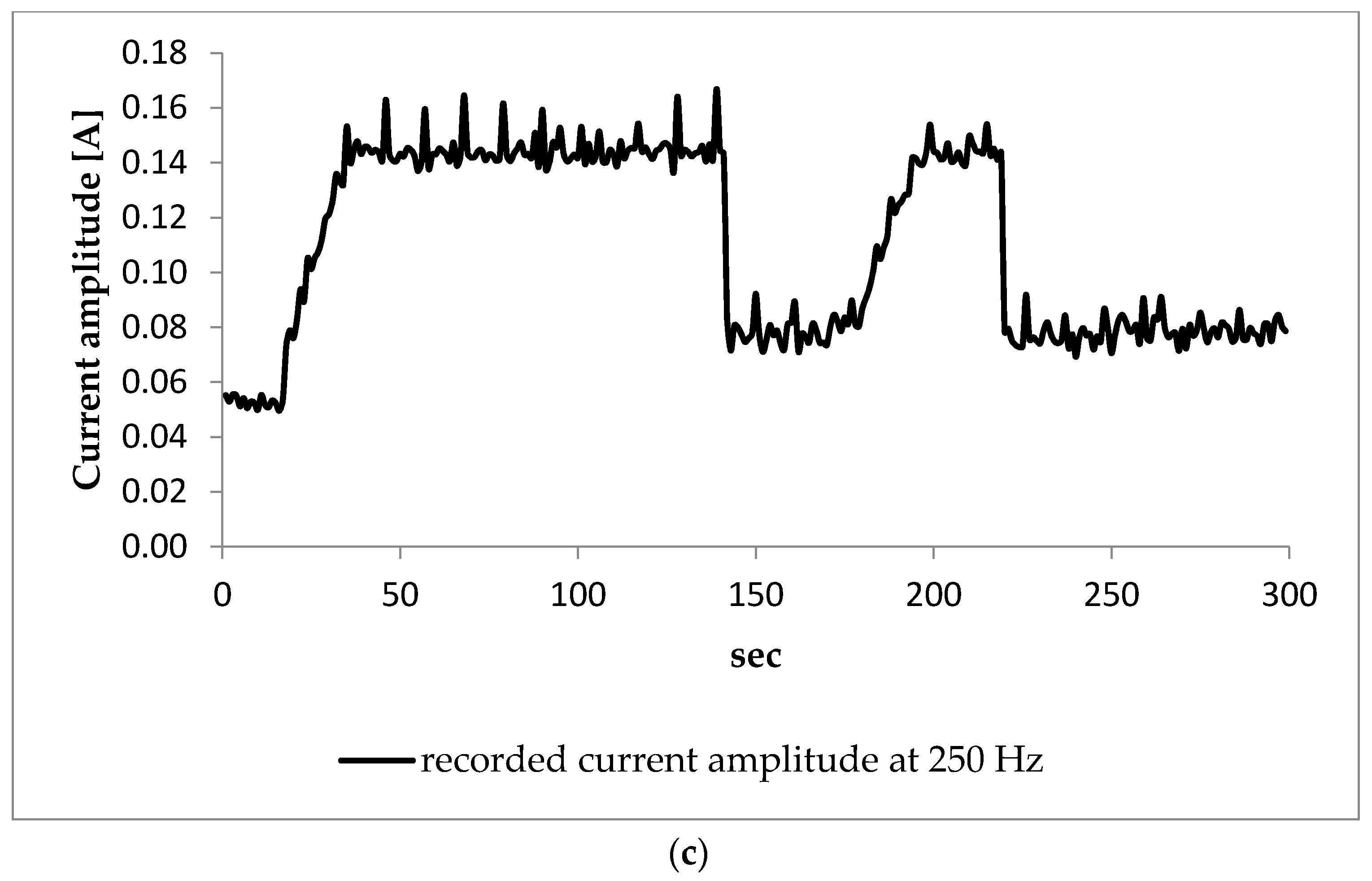
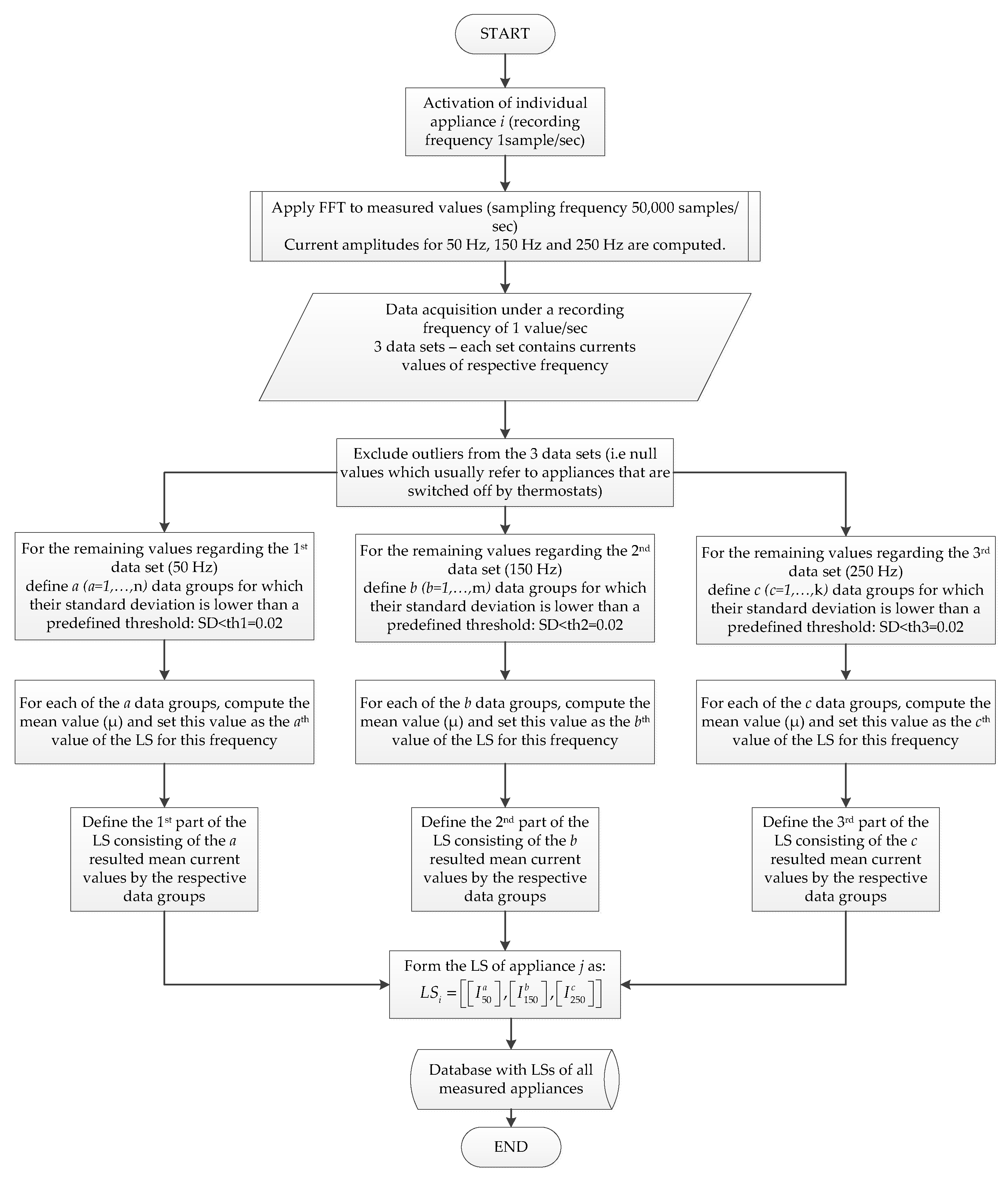
• Each appliance is measured for a time period of 5 min under a recording frequency of 1 sample/s as described in Section 2.1. Therefore, a data series with approximately 300 current values for each harmonic order (i.e., at 50 Hz, 150 Hz and 250 Hz) for each appliance are stored in the database. For most of the typical appliances in a residence the time period of 5 min can be considered adequate, since it captures the typical residential usage. For those with multiple operational modes, e.g., washing machine, all of these different operational modes should be measured, for the LS formulation.
• The standard deviation (SD) for each appliance is computed: SD₅₀, SD₁₅₀ and SD₂₅₀ respectively for the three examined frequencies.
• A threshold (th) is defined for each SD in order to identify if one or more values should be utilized for the formulation of the respective part of the LS.
• This threshold is taken as follows: SD_50(th) = SD_150(th) = SD_250(th) = 0.02. The value of the threshold (th) has been selected after several trials since this specific value has provided relatively short load signatures (i.e., with relatively few representative currents values) but efficient enough for load identification in the disaggregation mode of the proposed methodology. This threshold value is proposed as the upper limit regarding the data processing towards the LSs formulation.
• For each appliance i the following rules are applied:
  • If SD_50i ≤ SD_50(th), then compute the mean value (μ_50i) for the data in this data series and formulate the first part of the LS_i as follows: I_50i = μ_50i. Obviously in this case the value of index a is equal to 1, a = 1.
  • If SD_50i > SD_50(th), then reorder the data in the data series in descending order. Afterwards, divide top-down the data in a (a = 1, …, z) non-overlapping sequential data groups in order to ensure that for each one SD_50ia ≤ SD_50(th).
  • For each of these a groups, compute the mean value (μ_50ia). Formulate the first part of the LS_i as follows: I_50i = μ_50ia, …, μ_50iz.
  • Apply steps 5a–5c to the data series for 150 Hz and 250 Hz respectively under the corresponding SD threshold that is defined in step 4. This obtains the values of indices b and c.
  • Store the formulated LSs for the i appliances and form the LS database for this residence.

This procedure is summarized in the LS formulation flowchart of Figure 4.

Table 2. SD for data series of measured appliances.

Appliance	Recording Frequency 1 Value/S Recording Time Approximately 5 min
	SD50	SD150	SD250
PC-desktop	0.210	0.173	0.110
Hair dryer (hot)	0.031	0.005	0.011
Coffee maker 1	0.020	*	*
Vacuum	0.086	0.046	0.013
Electric iron 1	0.227	*	0.007
TV	0.010	0.006	0.007
Resistive Heater 1	0.039	*	0.020
Toaster 1	0.009	*	*
PC-laptop	0.165	0.107	0.032
Refrigerator	0.016	*	*
Blender	0.011	*	*

¹ data during deactivation (turned off) by thermostat excluded as outliers; * blank cells indicate negligible respective harmonic current.

illustrates the SDs resulted by the application of methodology described above, for all examined appliances and frequencies. These values provide an indication about the variance of the respective recorded current values under steady state operation. Finally, in

Table 3. LS database for the examined appliances.

LS Database for the Examined Residence
Appliance	1st Part for 50 Hz Current Amplitudes [A]		2nd Part for 150 Hz Current Amplitudes [A]		3rd Part for 250 Hz Current Amplitudes [A]		Indices Values a-b-c
PC (desktop)	1.122	1.154	1.078	1.022	0.818	0.739	10-10-9
	1.082	1.014	0.946	0.891	0.703	0.654
	0.940	0.865	0.856	0.774	0.579	0.516
	0.800	0.736	0.702	0.661	0.416	0.384
	0.630	0.588	0.563	0.522	0.346
Hair dryer (hot)	11.328	11.273	0.084		0.180 0.147		4-1-2
	11.162	11.136
Coffee maker	4.668	4.570	negligible		negligible		4-0-0
	4.425	4.389
Vacuum	6.588	6.514	1.281	1.228	0.123 0.100		8-5-2
	6.432	6.363	1.190	1.150
	6.300	6.225	1.134
	6.182	6.009
Electric iron	12.841	12.754	negligible		0.186		5-0-1
	12.687	12.598
	12.280
TV	0.100		0.175	0.142	0.167	0.150	1-2-2
Resistive Heater	14.940	14.805	negligible		0.234 0.202		4-0-2
	14.693	14.607
Toaster	2.721	2.670	negligible		negligible		2-0-0
Refrigerator	0.940	0.860	negligible		negligible		2-0-0
Blender	0.483	0.465	negligible		negligible		2-0-0

the resulted LS database for the examined residence is presented. It should be noted that the LSs for all appliances have been obtained by two set of measurements carried out in different days and times, in order to examine various measurement conditions such as the background. The result of the comparison between the measured data of different days is that the operating behavior for all appliances is consistent and do not vary significantly.

The magnitude of the threshold for the SD in each frequency, i.e., SD_50(th), SD_150(th) and SD_250(th), has a direct impact on the values of the a, b, c indices. Thus, the number of the values utilized for each of the three parts of the LS is also affected. Moreover, based on the results in Table 2, the PC, Electric iron and PC-laptop appliances seem to present the highest SD regarding their recorded current values. This high SD value is expected to increase the representative current values that will be utilized for the formulation of the appliance’s LS.

In order to be able to efficiently identify an operating appliance under aggregated simultaneous operation of various appliances, the LS of each appliance should be distinct and able to accurately reflect the operational behavior of each appliance. When recording each appliance for 5 min under state stated operation with a recording frequency of 1 value/s, then 300 current values are recorded for each harmonic order. Examining only the first three odd-harmonic orders, the recorded values for each appliance are 900 (i.e., 300 for 50 Hz, 300 for 150 Hz and 300 for 250 Hz). If for each harmonic order these 300 current values are the same, then obviously this value describes adequately the appliance’s behavior. However, if these values present variations, then a decision should be made about how many values should the signature contain, and how the signature should be formed. The goal is to be able to capture the appliance’s operational behavior under the most representative way and with the fewest possible current values. Using few representative current values for the LS formulation facilitates the identification procedure and reduces the computational burden during the disaggregation mode of the NILM algorithm. For example the complete LS for the TV appliance for could be in the form

$${\mathrm{LS}}_{TV}=\left[\left[I_{{50}_1},\mathrm{...},I_{{50}_{300}}\right],\left[I_{{150}_1},\mathrm{...},I_{{150}_{300}}\right],\left[I_{{250}_1},\mathrm{...},I_{{250}_{300}}\right]\right].$$

while using the proposed methodology the LS is reduced to:

$${\mathrm{LS}}_{TV}=\left[\left[0.1\right],\left[0.142,0.175\right],\left[0.15,0.167\right]\right]$$

This results in a shorter LS consisting of five values instead of 900 values.

2.4. Load Signatures of Agreggated Measurements

The core concept of the NILM methodologies relies on the following question:

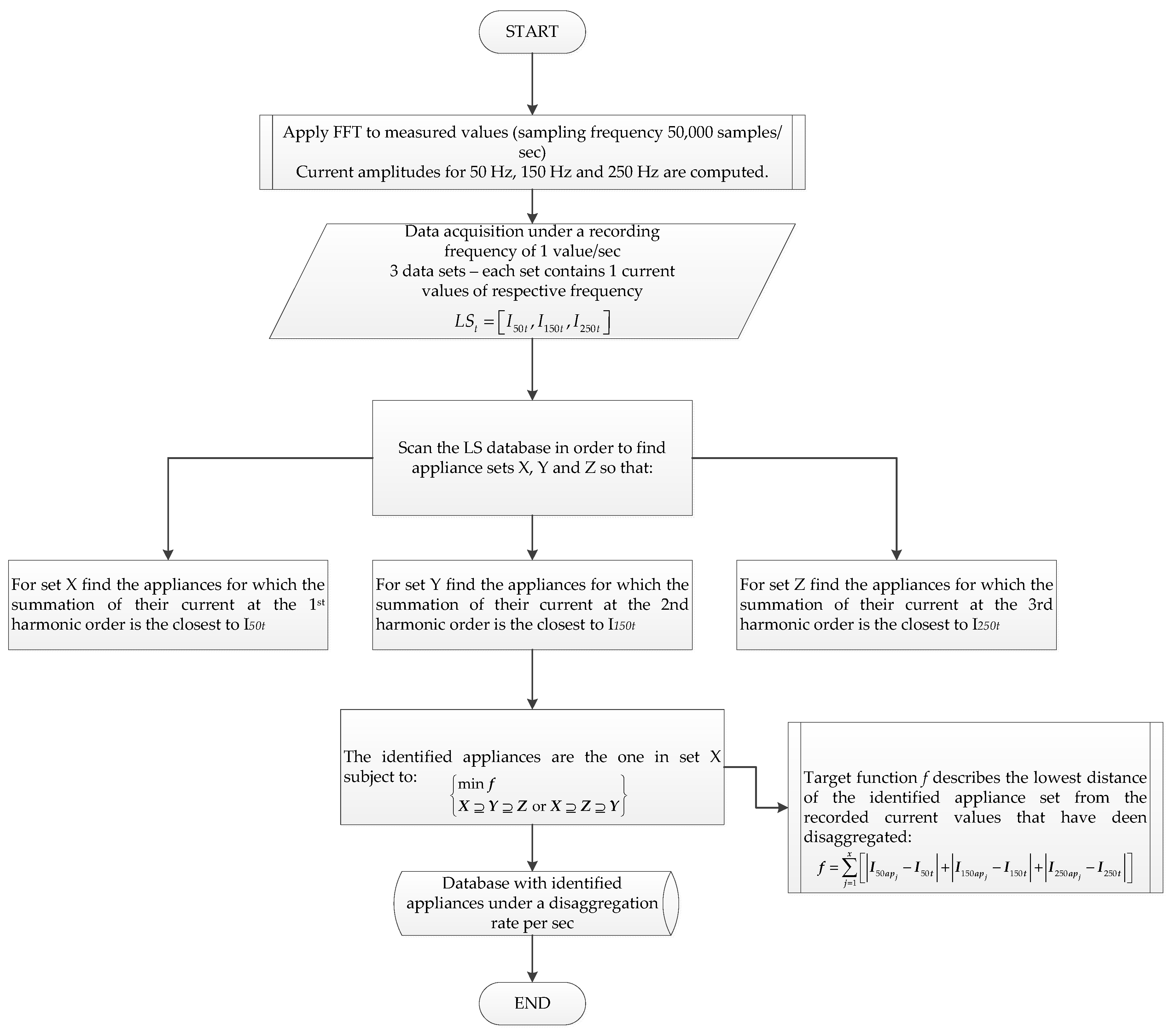
• Given a measurement of the total instantaneous current at the main feeding panel of the residence at time t, i.e., I_t, how could we identify the operating appliances in time t? Thus, the challenge here is to efficiently disaggregate the measured value to its components parts of certain loads.

In this work, the disaggregation procedure assumes that a measured aggregated current value at time t (minimum resolution for t is 1 s), results from the summation of the current values of each of the individual operating appliances. This simple linear approach is valid for the fundamental frequency of 50 Hz, i.e., the first part of the LS of each appliance. For the higher order harmonic currents the present analysis relies on the following:

A current harmonic magnitude (order h) concerning aggregated appliances may be determined by a generic law [28] as follows:

$$M_h=\sqrt[w]{{\displaystyle \sum _i{M}_{hi}^w}}$$

(2)

where M_h is the aggregated current harmonic at order h, M_hi is the current harmonic at order h of each appliance i, and w is an exponent that depends on the harmonic order. For h ≤ 5, w = 1. Hence, in this case, the aggregated harmonic current at order 3 or 5 is the sum of the respective harmonic currents injected by the appliances (i.e., linear approach). For higher harmonic orders the phase of the harmonic currents cannot be ignored, meaning that the harmonic currents should be formed as vectors. In this latter case, voltage measurements should also be performed and synchronized with the measurement of the instantaneous current in order to obtain the phase of each harmonic. The proposed methodology is simpler, since it relies only on current amplitudes measurements under a simpler measurement setup and data processing.

The LS of an aggregated measurement is formed under the same procedure that has been utilized for the LS database formulation in Section 2. Thus, for a given aggregated measured current value at time t, its load signature LS_t is formed as follows:

• Apply FFT to the measured instantaneous current values within time t
• Determine the current amplitudes for frequencies of 50 Hz, 150 Hz and 250 Hz
• The recorded values at time t is the mean of the current amplitudes

The LS_t is in the form that follows:

$${\mathrm{LS}}_t=\left[I_{50t},I_{150t},I_{250t}\right]$$

(3)

3. Proposed Methodology towards NILM Implementation

3.1. Disaggregation and NILM Algorithm

For the proposed NILM algorithm the identification of the unknown operating appliances could be summarized in the following problem:

Problem: Given a LS_t at any t, find the correct set of appliances for which the summation of the respective parts of the LSs best matches the corresponding part of LS_t. The mathematical formulation of this problem is as follows:

For i appliances (ap₁,…,ap_i) in the database find set X with x appliances $X=\left\{a{p}_1,\mathrm{...},a{p}_x\right\}$: minimize target function f $(\min f)$

where

$$f={\displaystyle \sum _{j=1}^x\left[\left|I_{50a{p}_j}-I_{50t}\right|+\left|I_{150a{p}_j}-I_{150t}\right|+\left|I_{250a{p}_j}-I_{250t}\right|\right]}\mathrm{and}x\le i$$

(4)

In order to decrease the computational burden of the disaggregation procedure, the solution space is cut down by applying the following procedure. The aim here is to filter/search the database in order to quickly determine the most possible candidate sets and then to define the correct set by applying (4) for the appliances it contains. Therefore, initially the sets X, Y, Z should be computed under the following constraints:

$$X=\left\{a{p}_1,\mathrm{...},a{p}_x\right\}\mathrm{with}x\mathrm{appliances}(x\le i):\left|{\displaystyle \sum _{j=1}^x{I}_{50j}^a}-I_{50t}\right|\le {\epsilon }_1$$

(5)

$$Y=\left\{a{p}_1,\mathrm{...},a{p}_y\right\}\mathrm{with}y\mathrm{appliances}(y\le i):\left|{\displaystyle \sum _{j=1}^y{I}_{150j}^b}-I_{50t}\right|\le {\epsilon }_2$$

(6)

$$Z=\left\{a{p}_1,\mathrm{...},a{p}_z\right\}\mathrm{with}z\mathrm{appliances}(z\le i):\left|{\displaystyle \sum _{j=1}^z{I}_{250j}^c}-I_{50t}\right|\le {\epsilon }_3$$

(7)

The correct set with the identified appliances should be set X:

$$\left\{\begin{array}{l}\min f\\ X\supseteq Y\supseteq Z\mathrm{or}X\supseteq Z\supseteq Y\end{array}\right\}.$$

Set X should always be a superset of sets Y and Z because current values have been recorded at 50 Hz for all appliances under steady state operation but not necessarily for 150 Hz and 250 Hz. It should be clarified that in this analysis ε₁ = ε₂ = ε₃ = 0.5.

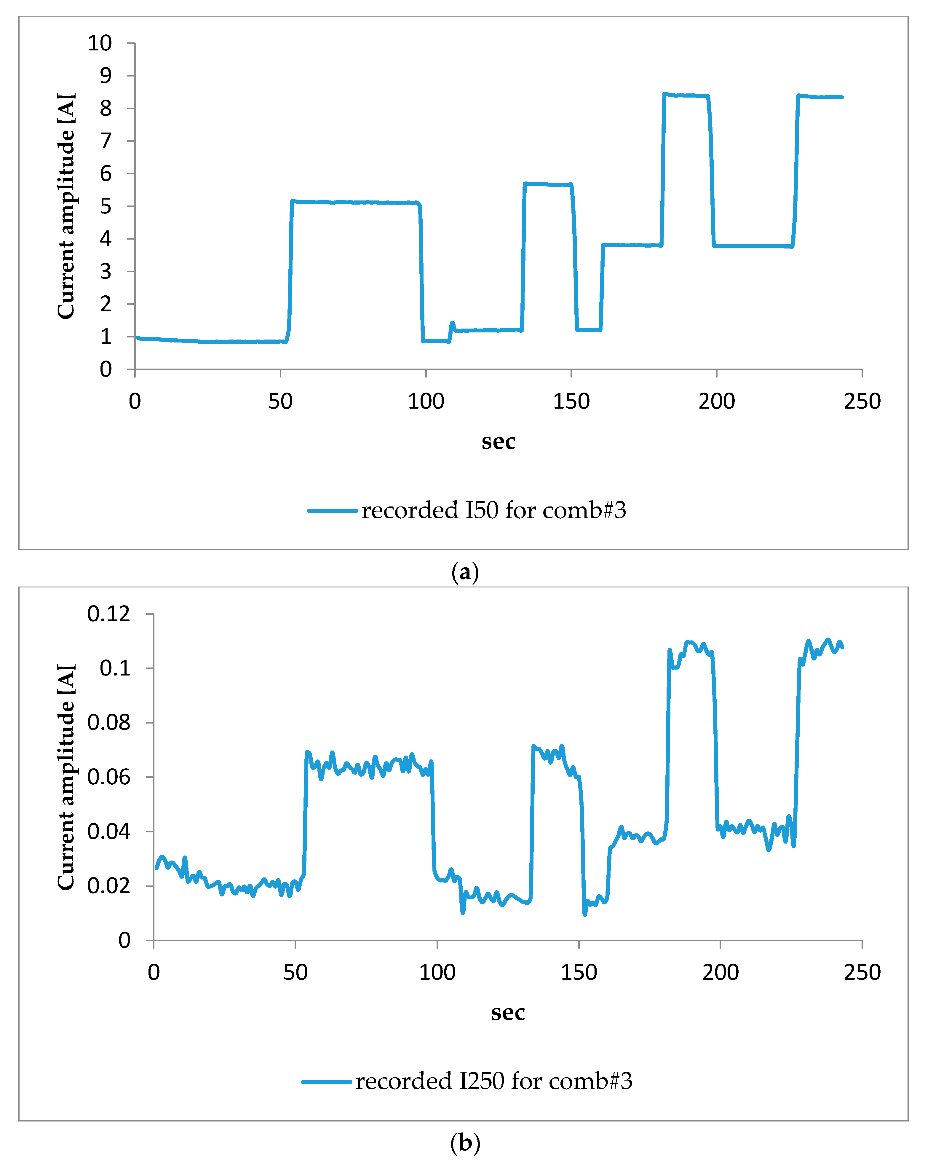
3.2. Disaggregation Results

The combinations that have been examined are presented in Table 1. The first combination (comb#1) consists of three appliances: (a) vacuum cleaner; (b) hair dryer; (c) resistive heater. The appliances were activated in sequential order at time steps of 1 min, in order to facilitate the demonstration of the disaggregation procedure. The latter has been applied to all examined combinations in this section. This combination has been selected due to the following reasons:

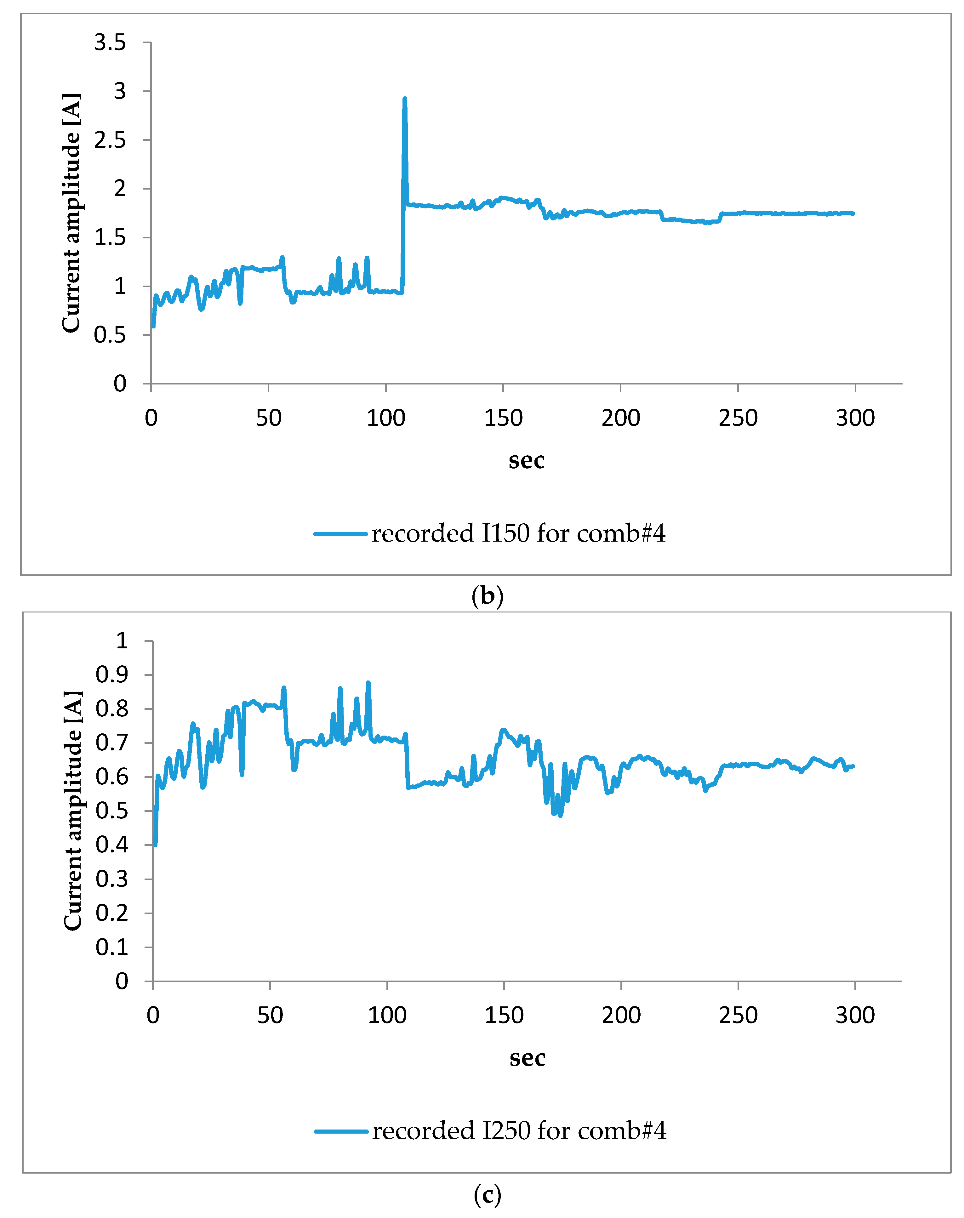
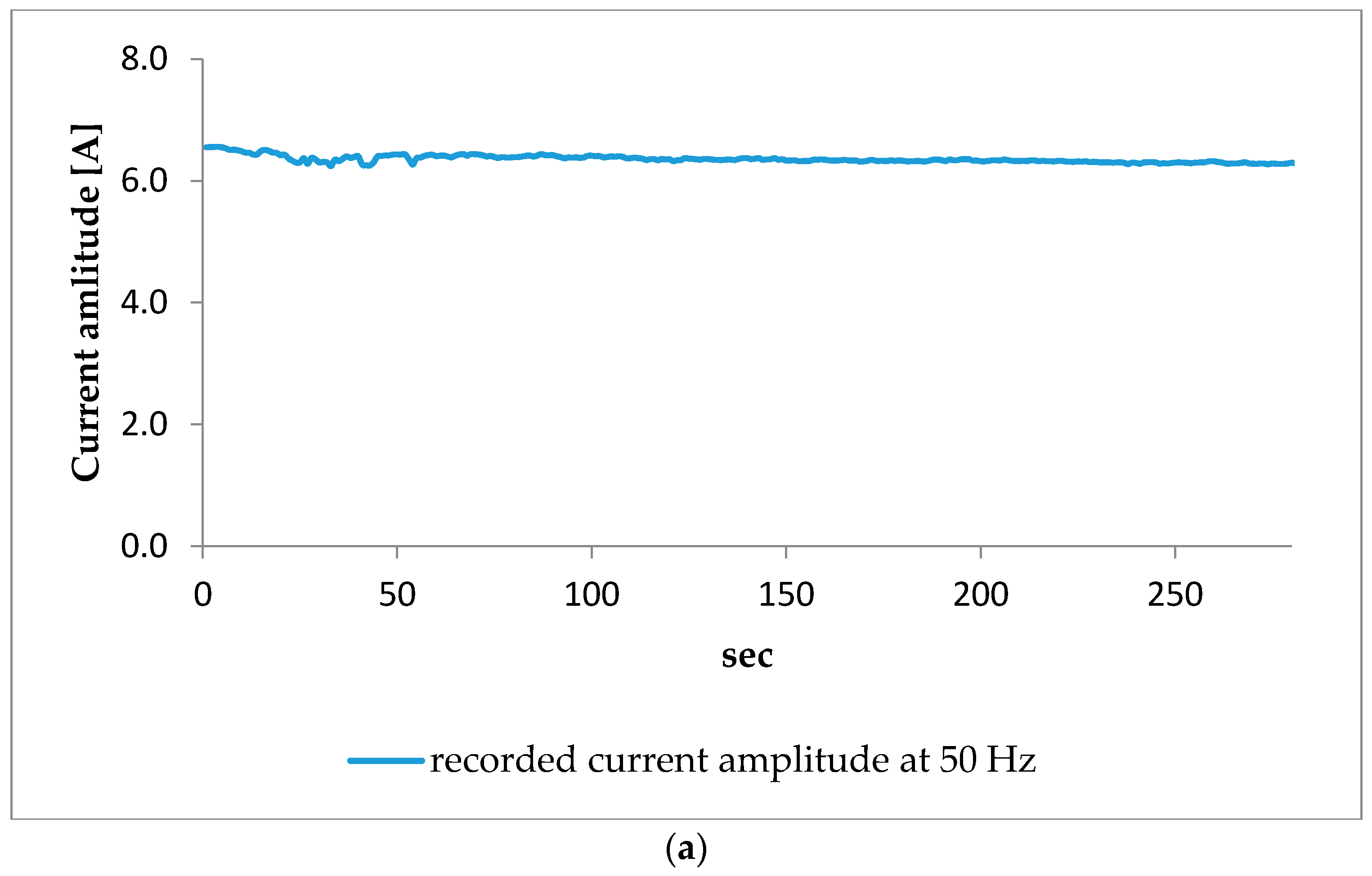
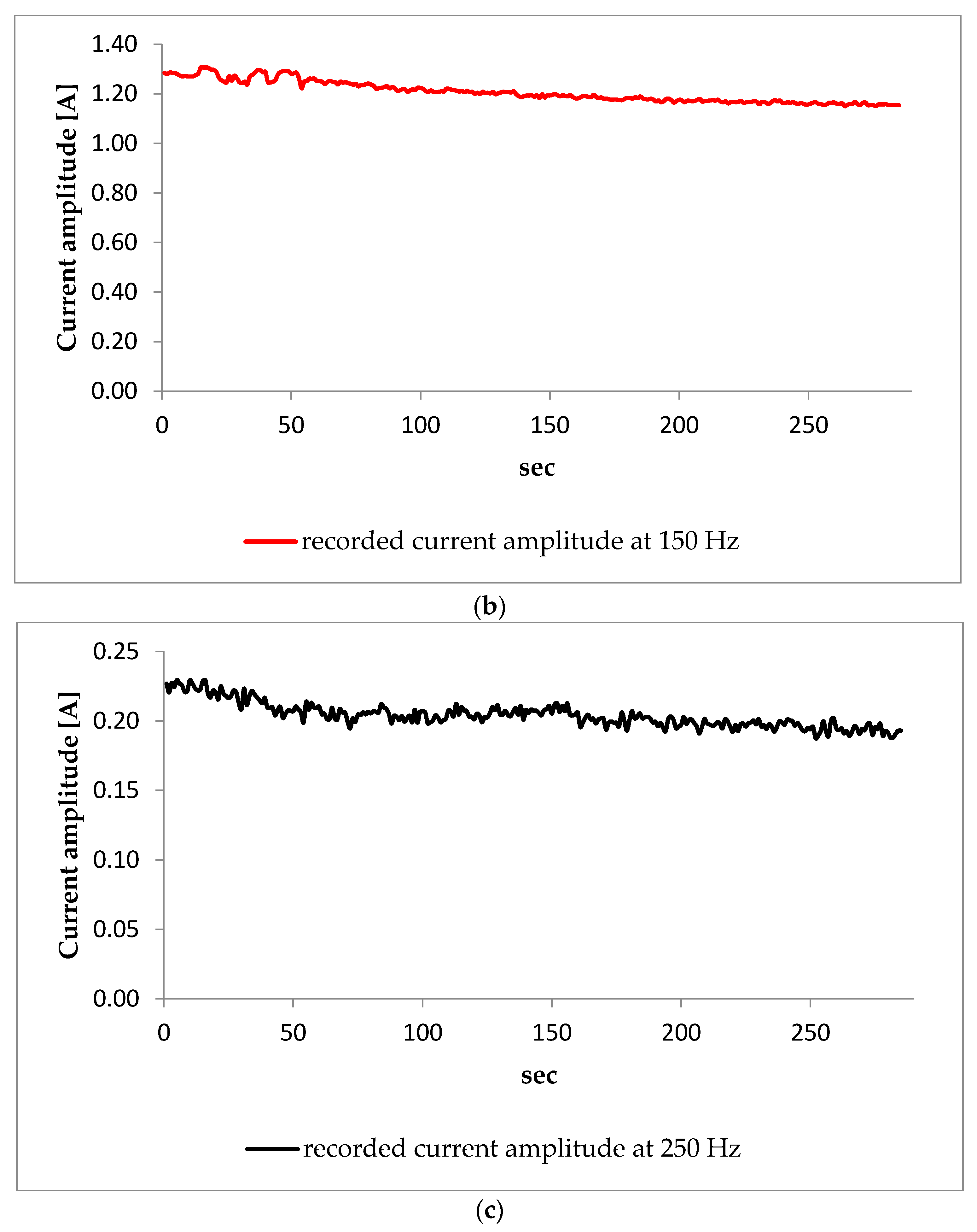
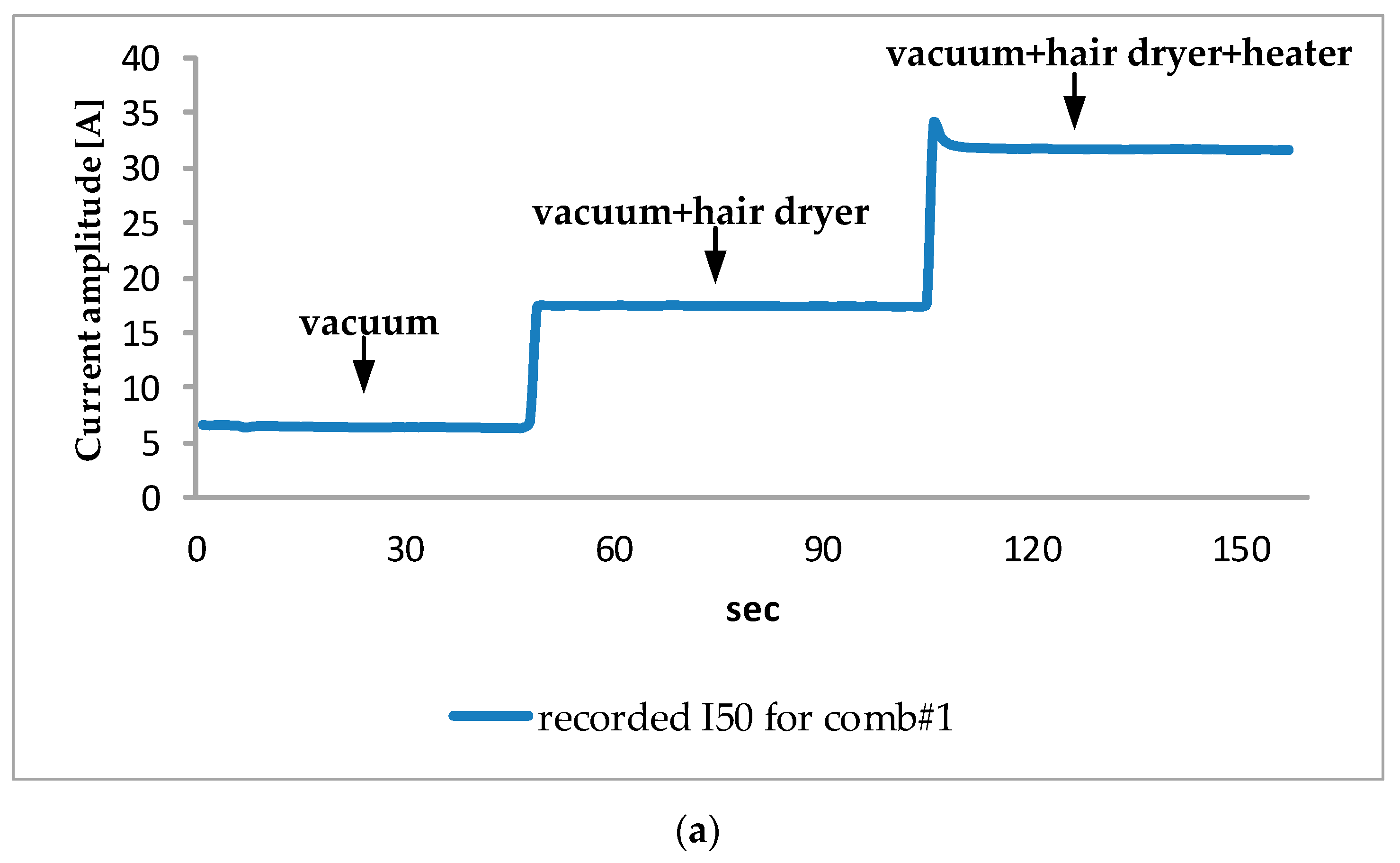
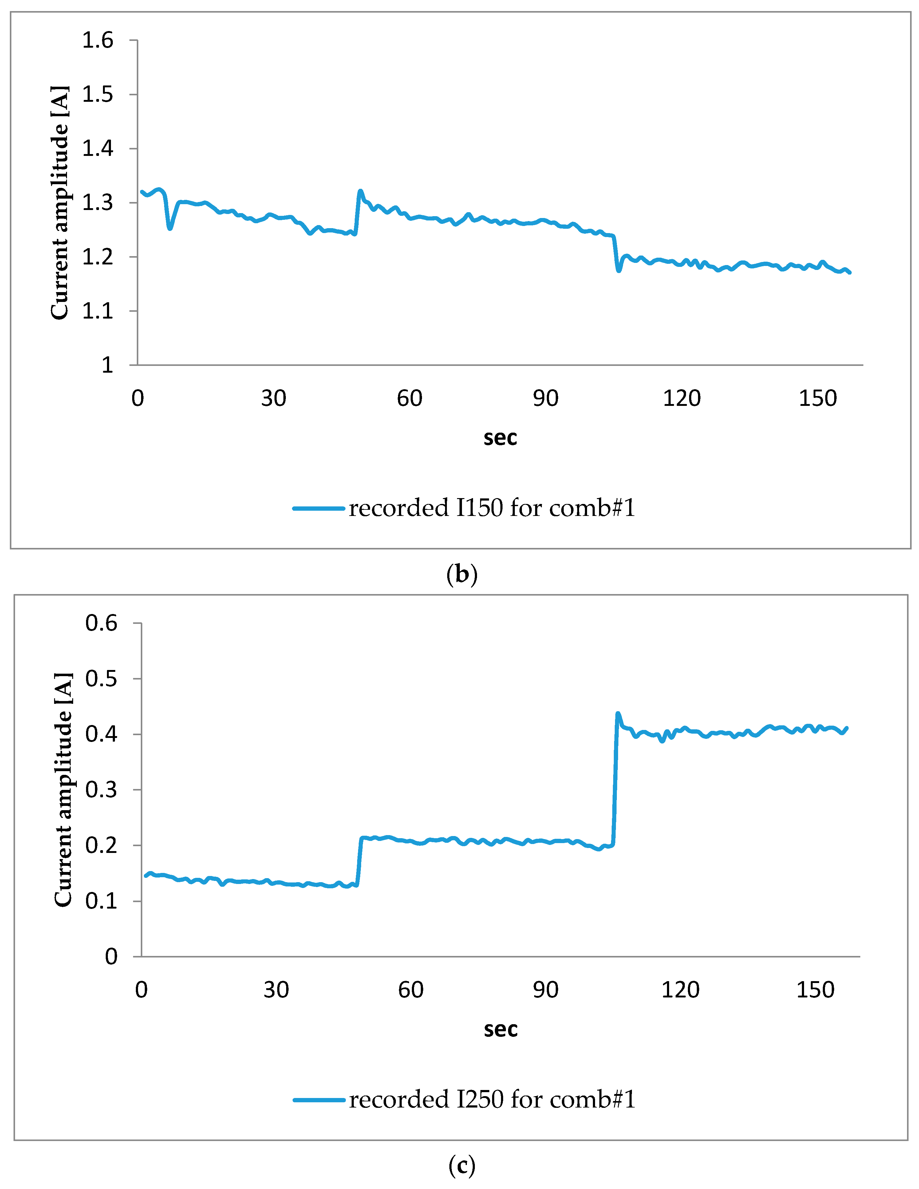
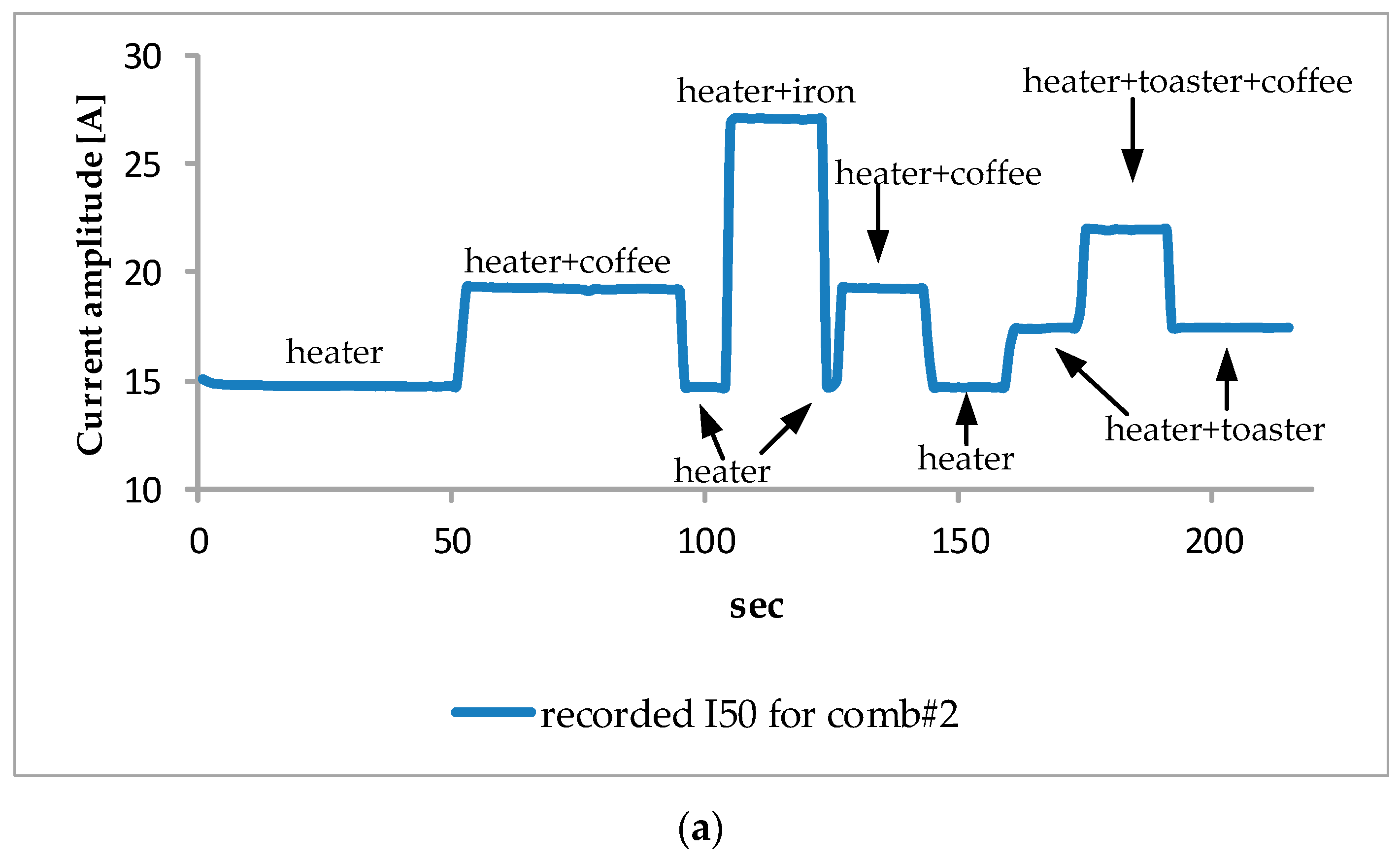
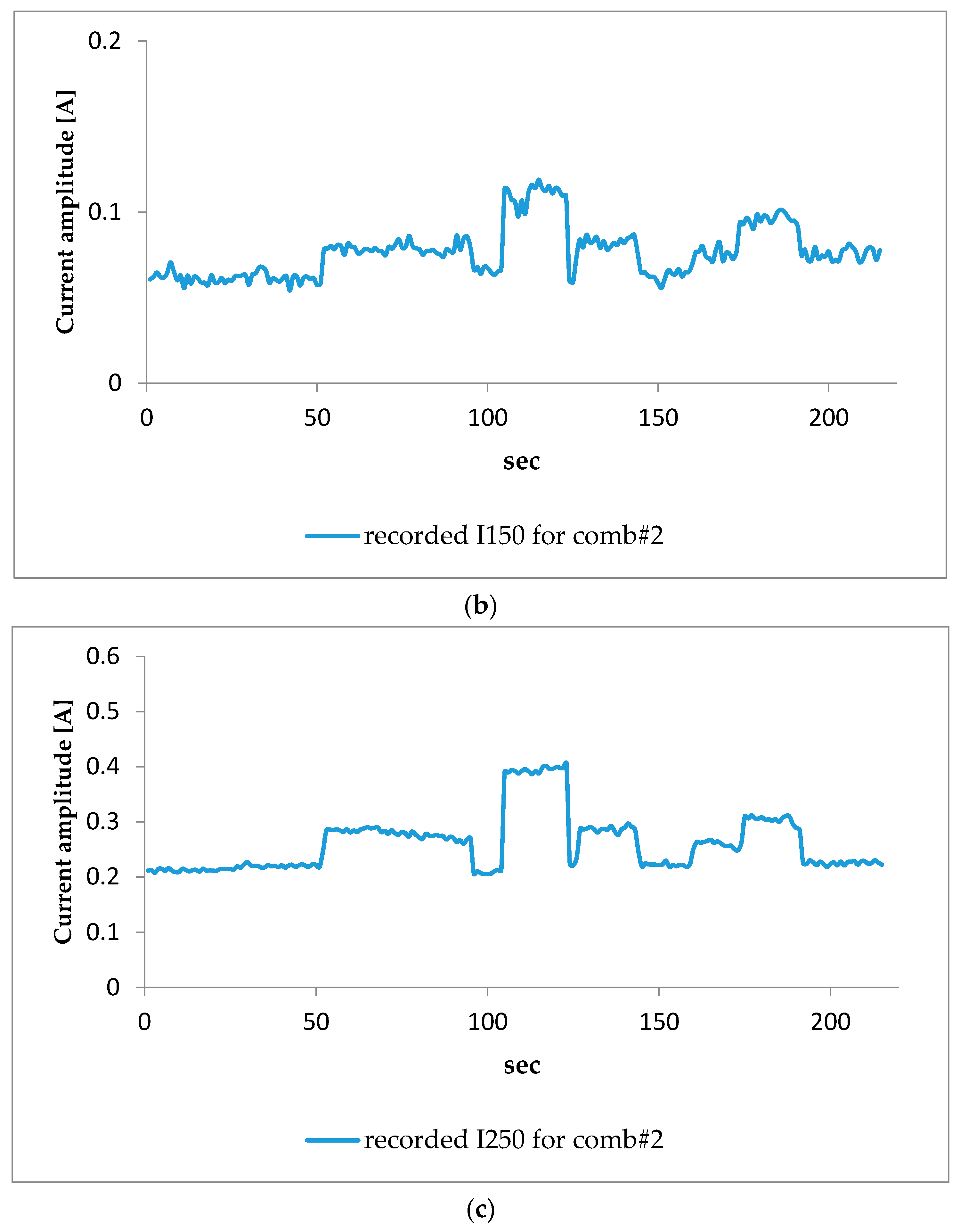
• Each appliance displays a relatively constant operational mode with smooth variations regarding the recorded current values.
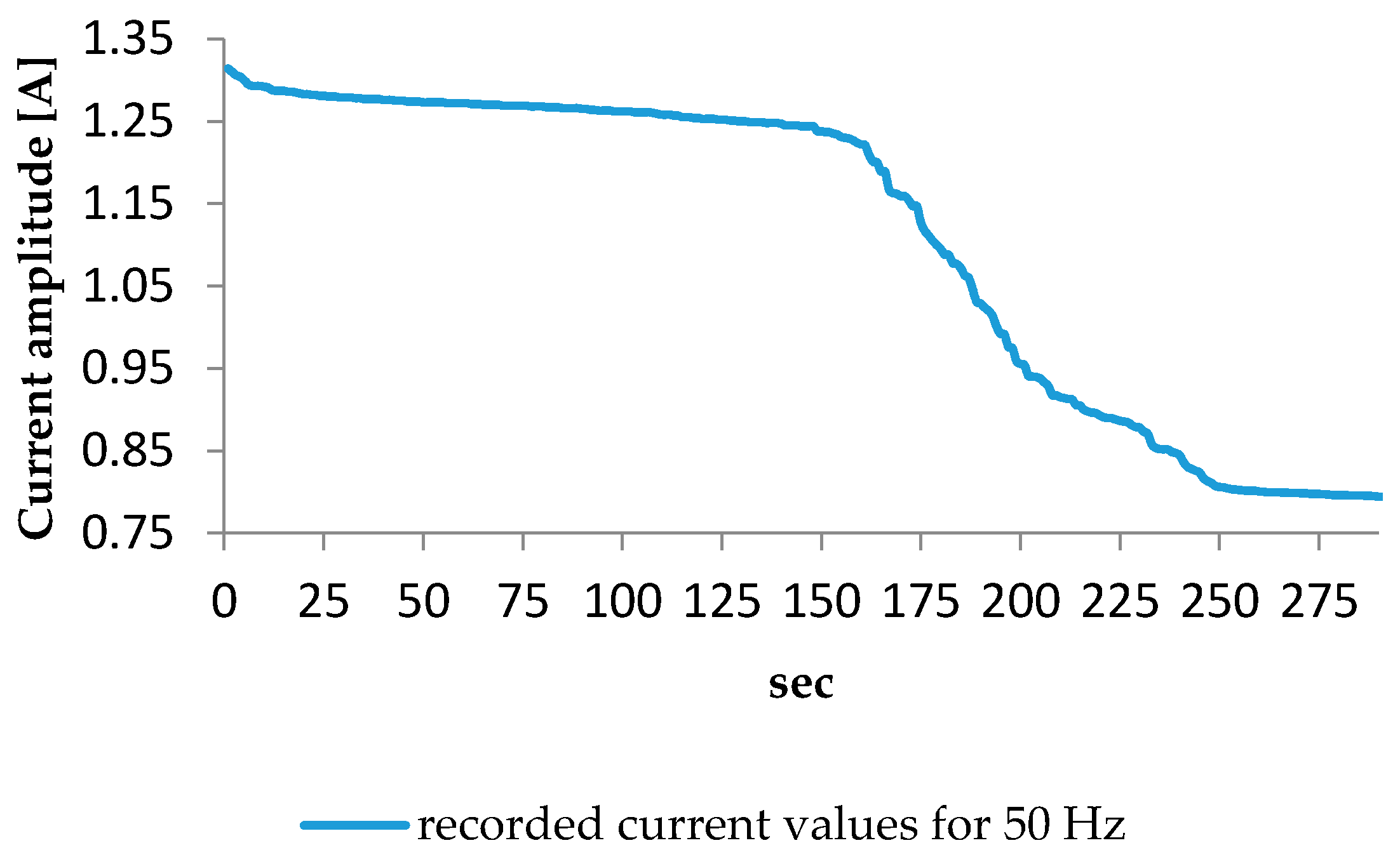
• Due to the high fundamental current of each appliance (i.e., I₅₀), when they operate simultaneously the variations of the aggregated fundamental current values could be higher than the current of small rated appliances. In this case the algorithm may incorrectly identify not operating appliances. Usually, such small rated appliances (e.g., TV or laptop) are not linear loads with significant 3rd and 5th order harmonic currents. Hence, in this case the OOHCs are expected to contribute by excluding these appliances from the identification procedure.

The loads are connected-activated sequentially in order to control the duration of appliances operating simultaneously (i.e., to know when each load has been activated and for how long it is operating). The latter is crucial during the disaggregation scheme since it enables the checking of the performance of the identification mode. When the second load is activated, the first one is still active, thus resulting in two appliances operating simultaneously. After the activation of the third load, three loads are operating simultaneously, and the same happens for the activation of the fourth load.

The second combination (comb#2) consists of the following three appliances: (a) resistive heater-coffee maker; (b) electric iron; (c) toaster. This set has been selected due to the fact that the operation of all appliances in the combination is ruled by thermostats. Thus, it is highly expected to record overlapping time periods regarding the activation-deactivation of the appliances.

The third combination (comb#3) consists of the following four appliances: (a) refrigerator; (b) coffee maker; (c) mixer; (d) toaster. This appliance set has been selected because it constitutes an excellent example of usual morning appliance operation related to breakfast preparation.

Finally, the fourth combination (comb#4) consists of five appliances, namely (a) PC; (b) TV; (c) vacuum cleaner; (d) heater and (e) iron. The interesting fact is that they all have OOHCs in their LSs and constitute a mix of small and large rated appliances.

In Figure 5a–c and Figure 6a–c the recorded current values for comb#1 and comb#2 are presented. It is clarified that the current values for the combinations are recorded per second and the NILM algorithm is applied accordingly. It should also be noted that the overlapping time periods regarding the activation-deactivation of the comb#2 is evident in Figure 6a for the current values at the fundamental frequency.

In Figure 7a,b and Figure 8a–c the recorded current values for comb#3 and comb#4 are also presented. It should be clarified that for comb#3 the recorded current values for the 3rd harmonic order was negligible.

In

Table 4. Disaggregation results and NILM performance.

comb#1
Appliance	Time Activated (s)	Correctly Identified (s)	NILM Performance	Min and Max Value of f
Vacuum	157	157	100%	0.044 0.423
Hair dryer (hot)	109	108	99%
Resistive heater	52	49	94%
comb#2
Resistive heater	215	208	97%	0.010 0.233
Coffee maker	78	78	100%
Electric iron	19	19	100%
Toaster	56	56	100%
2 times (at seconds 105 and 174) the algorithm identifies hairdryer-discarded.
comb#3
Refrigerator	243	195	80%	0.053 0.152
Coffee maker	97	97	100%
Blender	135	66	49%
Toaster	83	83	100%
failure to identify mixer is several cases—no irrelevant appliances proposed by the algorithm.
comb#4
PC (desktop)	300	163	54%	0.015 0.850
TV	240	0	0%
Vacuum	192	192	100%
Resistive heater	132	0	0%
Electric iron	24	24	100%
failure to identify TV (low current at 50 Hz falls within the variation ranges); failure to identify resistive heater due to the fact that Equation (2) was not valid for the aggregated current values of the 3rd and 5th harmonic currents.

the performance of the proposed NILM approach for the identification of the appliances for comb#1–comb#4 is illustrated. The performance is evaluated in terms of successful identification for each appliance per second. The latter is challenging since it could be considered to implement near real-time load identification. This is due to the fact that the NILM methodology is applied every second and the disaggregation scheme is performed in less than 1 s (the time varies but is always less than 1 s). Thus, the algorithm is fast enough to identify the operating appliances within the time frame of 1 s.

3.3. Results Evaluation

The basic conclusions derived by the results of Table 4 concerning the efficiency of the proposed LSs towards the NILM implementation are summarized below:

• The methodology for the LSs formulation could provide few and still representative current values that adequately cover the steady state operation of the appliances. A sensitivity analysis about the predefined SD threshold for each frequency could provide the optimal number of utilized current values for the formulation of the three parts of each LS.
• The proposed NILM scheme could be considered suitable for near real-time load identification. A NILM scheme with such high successful identification resolution could yield a detailed disaggregation of the consumption behavior of a residence and is highly appreciated by the retail energy providers. For example, the more detailed the knowledge of the consumption behavior of the customers the more efficiently demand response schemes can be designed and implemented.
• The identification approach performs almost flawlessly for combinations that include high consuming appliances without significant harmonic content. The latter is quite evident in comb#1 and comb#2 since Equation (2) is valid for the short LSs.
• For combinations with many appliances that present significant harmonic currents, the efficiency of Equation (2) is limited when only the harmonic current amplitudes are considered. In this case, the phase angle of each harmonic current should be also considered (using the fundamental voltage phase angle as the angular reference) because the aggregation should refer to vectors and not just amplitudes. For example, comb#4 includes five appliances that all present harmonic behavior. The summation of the harmonic current amplitudes shows high deviations from the considered recorded aggregated value of the combination. The latter explains the poor identification rate of the Resistive-heater appliance, since the algorithm identifies the Coffee-maker and Hair-dryer appliances instead. The problem here is that the contribution of the 5th harmonic current of the Resistive-heater is not identified in the aggregated recorded value. The TV appliance is not identified due to the same reason as well. Based on measurements in [29] the phase angle between the 5th harmonic currents of an LCD TV and a desktop PC is approximately 330°, thus the amplitudes should be almost subtracted concerning the aggregated respective amplitude under simultaneous operation.

In Figure 9 simple version of the flowchart regarding the disaggregation scheme of the proposed NILM algorithm is illustrated.

4. Conclusions

In this paper a novel approach regarding the implementation of a near real-time NILM algorithm is presented. The proposed methodology consists of two main parts: the first one analyzes the LS formulation and the second one the disaggregation scheme. For the former, only the current amplitudes at the fundamental frequency and the 3rd and 5th harmonic orders are utilized, while for the latter a simple disaggregation scheme is proposed. The analysis proposes the processing of the measured data of each appliance when operating individually in order to determine the most representative ones to be included in the LS.

Measurements have been performed under a developed measurement setup at the main feeding panel of a Low Voltage residence. Measurements included the stand-alone operation of the appliances for the formulation of the LS database, and four combinations concerning simultaneous operation of up to five appliances. For the four examined scenarios, involving different appliance combinations, the efficiency of the proposed methodology in terms of both the LS formulation and the disaggregation mode has been promising, even when the application rate is per second. More combinations should be examined in order to verify this finding. The disaggregation scheme follows a linear approach, thus, it is quite fast and appropriate for near real-time applications. The efficiency of the appliance identification is affected when the combinations include appliances with significant harmonic content. The problem in this case is that harmonic currents should be considered as vectors in order to properly account for their combined interaction in an aggregation mode. Therefore, in order to properly consider the summation of the harmonic currents we will examine the formulation of more efficient LSs under the consideration of the phase angles for the harmonic currents in a future work.

References

1. Paudyal, S.; Canizares, C.A.; Bhattacharya, K. Optimal Operation of Distribution Feeders in Smart Grids. IEEE Trans. Ind. Electron. 2011, 58, 4495–4503. [Google Scholar] [CrossRef]
2. Bouhouras, A.S.; Andreou, G.T.; Labridis, D.P.; Bakirtzis, A.G. Selective automation upgrade in distribution networks towards a smarter grid. IEEE Trans. Smart Grid 2010, 1, 278–285. [Google Scholar] [CrossRef]
3. Mehrshad, M.; Tafti, A.D.; Effatnejad, R. Demand side Management in the Smart Grid Based on Energy Consumption Scheduling by NSGA-II. Int. J. Eng. Pract. Res. 2013, 2, 197–200. [Google Scholar]
4. Chang, H.H.; Lin, C.L.; Lee, J.K. Load identification in nonintrusive load monitoring using steady-state and turn-on transient energy algorithms. In Proceedings of the 2010 14th International Conference on Computer Supported Cooperative Work in Design (CSCWD), Shanghai, China, 14–16 April 2010; pp. 27–32. [Google Scholar]
5. Liang, J.; Ng, S.K.K.; Kendall, G.; Cheng, J.W.M. Load signature studypart I: Basic concept, structure, and methodology. IEEE Trans. Power Deliv. 2010, 25, 551–560. [Google Scholar] [CrossRef]
6. Hart, G.W. Nonintrusive Appliance Load Monitoring. Proc. IEEE 1992, 80, 1870–1891. [Google Scholar] [CrossRef]
7. Laughman, C.; Lee, K.; Cox, R.; Shaw, S.; Leeb, S.; Norford, L.; Armstrong, P. Power signature analysis. IEEE Power Energy Mag. 2003, 1, 56–63. [Google Scholar] [CrossRef]
8. Lin, Y.-H.; Tsai, M.-S. A novel feature extraction method for the development of nonintrusive load monitoring system based on BP-ANN. In Proceedings of the 2010 International Symposium on Computer, Communication, Control and Automation, Tainan, Taiwan, 5–7 May 2010; Volume 2, pp. 215–218. [Google Scholar]
9. Yang, H.T.; Chang, H.H.; Lin, C.L. Design a neural network for features selection in non-intrusive monitoring of industrial electrical loads. In Proceedings of the 2007 11th International Conference on Computer Supported Cooperative Work in Design (CSCWD), Melbourne, Australia, 26–28 April 2007; pp. 1022–1027. [Google Scholar]
10. Ng, S.K.K.; Liang, J.; Cheng, J.W.M. Automatic appliance load signature identification by statistical clustering. In Proceedings of the 8th International Conference on Advances in Power System Control, Operation and Management (APSCOM 2009), Hong Kong, China, 8–11 November 2009; pp. 1–6. [Google Scholar]
11. Chang, H.H.; Chen, K.; Tsai, Y.P.; Lee, W.J. A New Measurement Method for Power Signatures of Nonintrusive Demand A New Measurement Method for Power Signatures of Nonintrusive Demand Monitoring and Load Identification. IEEE Trans. Ind. Appl. 2012, 48, 764–771. [Google Scholar] [CrossRef]
12. Du, Y.; Du, L.; Lu, B.; Harley, R.; Habetler, T. A review of identification and monitoring methods for electric loads in commercial and residential buildings. In Proceedings of the 2010 IEEE Energy Conversion Congress and Exposition (ECCE), Atlanta, GA, USA, 12–16 September 2010; pp. 4527–4533. [Google Scholar]
13. Shao, H.; Tech, V.; Marwah, M. A Temporal Motif Mining Approach to Unsupervised Energy Disaggregation. In Proceedings of the 1st International Workshop on Non-Intrusive Load Monitoring, Pittsburgh, PA, USA, 7 May 2012; pp. 1–2. [Google Scholar]
14. Li, J.; Yang, H. The investigation of residential load identification technologies. In Proceedings of the 2012 Asia-Pacific Power and Energy Engineering Conference (APPEEC), Shanghai, China, 27–29 March 2012; pp. 2–5. [Google Scholar]
15. Srinivasan, D.; Ng, W.S.; Liew, A.C. Neural-network-based signature recognition for harmonic source identification. IEEE Trans. Power Deliv. 2006, 21, 398–405. [Google Scholar] [CrossRef]
16. Ehrhardt-martinez, A.K.; Donnelly, K.A. Advanced Metering Initiatives and Residential Feedback Programs: A Meta-Review for Household Electricity-Saving Opportunities. Energy 2010, 123, 128. [Google Scholar]
17. Chang, H.H. Non-intrusive demand monitoring and load identification for energy management systems based on transient feature analyses. Energies 2012, 5, 4569–4589. [Google Scholar] [CrossRef]
18. Bacurau, R. Experimental Investigation on the Load Signature Parameters for Non-Intrusive Load Monitoring. Prz. Elektrotech. 2015, 1, 88–92. [Google Scholar] [CrossRef]
19. Hong, Y.Y.; Chou, J.H. Nonintrusive energy monitoring for microgrids using hybrid self-organizing feature-mapping networks. Energies 2012, 5, 2578–2593. [Google Scholar] [CrossRef]
20. Zoha, A.; Gluhak, A.; Imran, M.A.; Rajasegarar, S. Non-intrusive Load Monitoring approaches for disaggregated energy sensing: A survey. Sensors 2012, 12, 16838–16866. [Google Scholar] [CrossRef] [PubMed]
21. Huang, S.J.; Hsieh, C.T.; Kuo, L.C.; Lin, C.W.; Chang, C.W.; Fang, S.A. Classification of home appliance electricity consumption using power signature and harmonic features. Proceedings of 2011 IEEE Ninth International Conference on Power Electronics and Drive Systems, Singapore, 5–8 December 2011; pp. 596–599. [Google Scholar]
22. Bouhouras, A.S.; Milioudis, A.N.; Andreou, G.T.; Labridis, D.P. Load signatures improvement through the determination of a spectral distribution coefficient for load identification. In Proceedings of the 2012 9th International Conference on the European Energy Market (EEM), Florence, Italy, 10–12 May 2012; pp. 1–6. [Google Scholar]
23. Bouhouras, A.S.; Milioudis, A.N.; Labridis, D.P. Development of distinct load signatures for higher efficiency of NILM algorithms. Electr. Power Syst. Res. 2014, 117, 163–171. [Google Scholar] [CrossRef]
24. Semwal, S.; Shah, G.; Prasad, R.S. Identification residential appliance using NIALM. In Proceedings of the 2014 IEEE International Conference on Power Electronics, Drives and Energy Systems, Mumbai, India, 16–19 December 2014. [Google Scholar]
25. Srinivasan, G.; Anandan, C.; Jain, S.A.K.; Ahmed, S.S.; Vijayaraghavan, V. Low-cost Non-Intrusive Device Identification System. In Proceedings of the 2016 IEEE Circuits and Systems Conference (DCAS), Arlington, TX, USA, 10 October 2016; pp. 4–7. [Google Scholar]
26. Feng, C.Y.; Hoe, H.M.; Abdullah, P. Tracing of Energy Consumption by Using Harmonic Current. In Proceedings of the 2013 IEEE Student Conference on Research and Development (SCOReD), Putrajaya, Malaysia, 16–17 December 2013; pp. 16–17. [Google Scholar]
27. Tran, T.T.; Lee, G.-D.; Pham, T.X.; Kim, G.-J.; Van Dang, C.; Kim, J.-W.; Kang, B. Identification of In-Home Appliances Through Analysis of Current Consumption. In Proceedings of the 10th International Conference on Ubiquitous Information Management and Communication, Danang, Vietnam, 4–6 January 2016. [Google Scholar]
28. Gil-de-castro, A.; Moreno-muñoz, A. Street Lamps Aggregation Analysis through IEC 61000-3-6 Approach. In Proceedings of the 22nd International Conference on Electricity Distribution, Stockholm, Sweden, 10–13 June 2013; pp. 10–13. [Google Scholar]
29. Nassif, A.B.; Yong, J.; Xu, W.; Chung, C.Y. Indices for comparative assessment of the harmonic effect of different home appliances. Eur. Trans. Electr. Power 2014, 23, 638–654. [Google Scholar] [CrossRef]
Figure 1. (a) Recorded current amplitudes for laptop appliance for 50 Hz; (b) Recorded current amplitudes for laptop appliance for 150 Hz; (c) Recorded current amplitudes for laptop appliance for 250 Hz.
Energies 10 00538 g001aEnergies 10 00538 g001b
Figure 2. (a) Recorded current amplitudes for vacuum appliance for 50 Hz; (b) Recorded current amplitudes for vacuum appliance for 150 Hz; (c) Recorded current amplitudes for vacuum appliance for 250 Hz.
Energies 10 00538 g002aEnergies 10 00538 g002b
Figure 3. Recorded current amplitudes for PC (desktop) appliance for 50 Hz.
Energies 10 00538 g003
Figure 4. Proposed methodology flowchart for LS formulation.
Energies 10 00538 g004
Figure 5. (a) Recorded current values I50 for comb#1; (b) Recorded current values I150 for comb#1; (c) Recorded current values I250 for comb#1.
Energies 10 00538 g005aEnergies 10 00538 g005b
Figure 6. (a) Recorded current values I50 for comb#2; (b) Recorded current values I150 for comb#2; (c) Recorded current values I250 for comb#2.
Energies 10 00538 g006aEnergies 10 00538 g006b
Figure 7. (a) Recorded current values I50 for comb#3; (b). Recorded current values I250 for comb#3.
Energies 10 00538 g007
Figure 8. (a) Recorded current values I50 for comb#4; (b) Recorded current values I150 for comb#4; (c) Recorded current values I250 for comb#4.
Energies 10 00538 g008aEnergies 10 00538 g008b
Figure 9. Flowchart for the disaggregation scheme of the proposed NILM algorithm.
Energies 10 00538 g009