Reliability Assessment of Power Generation Systems Using Intelligent Search Based on Disparity Theory

Abstract

The reliability of the generating system adequacy is evaluated based on the ability of the system to satisfy the load demand. In this paper, a novel optimization technique named the disparity evolution genetic algorithm (DEGA) is proposed for reliability assessment of power generation. Disparity evolution is used to enhance the performance of the probability of mutation in a genetic algorithm (GA) by incorporating features from the paradigm into the disparity theory. The DEGA is based on metaheuristic searching for the truncated sampling of state-space for the reliability assessment of power generation system adequacy. Two reliability test systems (IEEE-RTS-79 and (IEEE-RTS-96) are used to demonstrate the effectiveness of the proposed algorithm. The simulation result shows the DEGA can generate a larger variety of the individuals in an early stage of the next population generation. It is also able to estimate the reliability indices accurately.

1. Introduction

One of the main challenges when planning power demand is evaluating the reliability of the generating system adequacy. Even though a considerable number of research have been carried out in the area of generating system reliability, there is still need for more suitable techniques that are more realistic and computationally flexible to represent the power generating adequacy [1,2,3,4].

Numerous new, robust computational intelligence techniques that are widely used in power system applications have been previously described by [5]. These techniques are often utilized to solve complex problems in power systems, which are difficult to solve with conventional methods. The objective of using metaheuristic optimization techniques is to present new algorithms that can solve complicated reliability analysis for electrical power systems, such as the increase in the complexity of the power systems infrastructure, low accuracy for reliability indices estimates, and large computation effort.

Many optimization algorithms have been developed utilizing the nature of population-based intelligent research; these algorithms use all possible solutions by iteratively and stochastically changing rather than focusing on improving a single solution. Examples of these algorithms include the ant colony system (ACS), genetic algorithm (GA), particle swarm optimization (PSO), intelligent state space pruning (ISSP), and evolutionary computation (EC) [6,7,8,9,10].

The GA is often selected to assess the reliability indices of the generating system so that the representations of most of the system expectation states can be easily encoded in binary maps. The GA can be defined as one of the metaheuristic search algorithms, which is based on biological evolution. It utilizes one form of the three parameters of selection, crossover, and mutation when implemented. Based on the optimization research mechanism, GA is utilized to scan, as well as to discover a particular failure state that has the most significant contribution to the assessment indices of the adequacy of the entire system.

Application of GA will reduce the search space and computational efforts in calculating reliability indices of a generating and composite system [11]. GA has the ability to locate failure states in a more effective manner, compared to the other conventional approach, whereby each sampling state for the power system represents a deficiency in the power system capacities.

There are many ways to implement a GA, such as implementing the modified GA using the state space pruning tool to scan the failure state of the system and calculating the reliability indices with Monte Carlo simulation (MCS) [12,13]. It was reported that these algorithms perform better than when only the analysis methods or the MCS are used. However, such an algorithm requires a longer computation period when the population size is too large [14]. The modified simple genetic algorithm (MSGA) approach has also been proposed [15,16]. It was utilized as a tool for sampling that could construct the generation system state array which represents the failure states of the system. To determine the adequacy indices of generating systems, convolution was carried out between load profiles and the state array of power generating states.

A listed series of aspects may or may not be customized to affect the diversity in the population through the spreading of the same individuals [10], leading to deceleration of evolution speed. In the MSGA approach, accurate results can be obtained by selecting suitable parameters, such as mutation probability, population size, and crossover probability. This procedure showed that the algorithm was not strongly dependent on the population size or crossover probability, but was affected by mutation probability. Furthermore, lower mutation probability values lead to high errors, while increased mutation probability values result in more errors because the search process is converted into a random search. Therefore, the efficient selection of the probability of mutation can lead to a significant improvement in the population fitness of the genetic algorithm.

The technique uses a GA as a search tool to find the most probable system failure states. In this paper, a novel DEGA is proposed, which is a combination of disparity theory and genetic algorithms. The developed technique can improve the simple genetic algorithm by increasing the generation of failure states of the system to provide a good approximation of the calculated reliability indices. An interesting feature of this technique is the accelerated evolution velocity, through the application of the variety of the probability of mutation. Thus, the number of failure states that are created by this algorithm are larger than the failure states obtained by the GA. In conclusion, the benefits of using the intelligent search techniques, is that an accurate assessment of reliability indices for the power generation system with less computational effort can be obtained. So far, the proposed method has shown to be efficient in obtaining an accurate evaluation of reliability indices, and reducing the computational burden, as compared to other algorithms used for the same purpose.

2. Related Work

2.1. Reliability Assessment of the Generating System

The reliable power supply has always been an important aspect in the electric generating system adequacy for future system capacity expansion. This is to ensure that the total installed capacity is sufficient to provide adequate electricity when needed. Consequently, the electric generating system may utilize one or more quantitative risk reliability indices as part of the criteria to decide the system risk model. The fundamental reliability indices evaluated in this paper are adopted to enable the estimation of the reliability level of the power generating systems; these comprise of, loss of load frequency (LOLF), loss of energy expectation (LOEE) and, loss of load expectation (LOLE).

The two main modes by which the load model is generally represented are chronological and non-chronological. Both of these modes can be used along with different intelligent search techniques. For example, the load duration curve (LDC) will generate values for each hour, hence, there will be (8736) individual values recorded for each year, conversely, the daily peak load variation curve (DPLVC) will generate (365) values for the year [17].

The chronological load sequence (N_t), is represented within this study, and the L_i, represents the discrete values for successive time for different levels of load, (I = 1, 2... N_t). Each one of these time steps possesses an equation that is equal, (t = t/N_t), where (t) represents the entire observation period for the load levels. As each time step takes one hour, the equation below can be used to calculate the LOLE (in hours) within the observation horizon (t):

$$\mathrm{LOLE}={\displaystyle \sum }_{i=1}^{N_t}{P}_{f_i}$$

(1)

The calculation for (LOEE) in megawatts hour is:

$$\mathrm{LOEE}={\displaystyle \sum }_{i=1}^{N_t}PN{S}_i$$

(2)

where PNS_i, is the power not supplied, and P_fi represents the load probability lost for hour t.

LOLF is defined as the frequency of a failure state, which involves two main components; the first component is frequency due to load fluctuation “FL”, due to load level transition from its current state to another load state, and the second component is the frequency of the generating system capacity “FG”, due to transition of generation units (probability of the capacities outage). The calculation for the LOLF that occurs throughout the time span of the observation is:

$$\mathrm{LOLF}=FG+FL$$

(3)

where FL is the frequency of the component due to the load fluctuation, which is caused by the uncertainty of the system demand, and FG is the frequency due to the uncertainty failure of conventional generating units for supplying the power [11].

2.2. Modified Simple Genetic Algorithm (MSGA)

A genetic algorithm is one of the most powerful and primary methods that can be applied as a stochastic search tool, and an optimization technique based on the concepts of evolution theory. Compared with other search methods, the GA is programmed to find the best solution to the search problem with respect to other search methods, such as the MCS and analysis methods for assessing the generating system reliability. Still, there are imperfections in the searching performance during the beginning and final stages of the GA due to the parameters of genetics. Mostly, the GA parameters include the normal constant rates for mutation, selection, and crossover rate [18]. Figure 1 illustrates the flow of GA.

On the other hand, according to Samaan and Singh [16], an MSGA is not significantly affected by initial population size or probability crossover (P_c), but it can be significantly affected by the probability of the permutation (P_m). Meanwhile, low values of P_m can result in a high number of errors, due to premature identifications of failure state probabilities. This condition decreases the probability of generating new states (i.e., similar individuals tend to be diffused into next generation populations). At the same time, errors can be increased with higher values of P_m. Consequently, such a condition can conjure a random search from the search process (increases the diversity of solutions, caused by a large number of evolutions in the P_m).

2.3. State Space

The state space in a power system consists of all possible states of components or generating units. The representation of each conventional generating unit in the system is conducted by, using a two-state model. In the Markovian two-state model, each unit can only have the success and failure states, while the generating units are regarded as either being completely out of service (down) or totally in service (up). Both the MCS and PIS (population-based intelligent search) methods have the state spaces, but are different in their mechanisms for sampling; with regards to MCS, the state of success or failure influences the reliability indices estimation. This implies that the sampling of the state of failure is less likely compared to the state of success. This condition explains why the convergence takes more computation effort in the reliability assessment of highly reliable systems. Meanwhile, for PIS, the system state of the failure probability system can guide the search [19]. Therefore, the state of a system that has a higher probability of failure can ensure greater chances to be nominated and evaluated. To date, this characteristic has enabled the PIS algorithms to be utilized to address various complex problems due to its higher efficiency.

3. The Proposed Method

3.1. DEG Algorithm

Figure 2 describes the proposed method, DEGA, which comprises of an improved mutation operator which adopts the modeling disparity theory of evolution as its method of the reproduction of genes.

According to this theory, the chromosome has two strands, the first is the one with low rates of mutation which is called the leading strand (le) and the second, one with high mutation rates is called the lagging strand (la). Figure 3 illustrates these two models.

By using DEGA, one parent’s chromosome can create two children, which occurs from the mutation of the (le) and (la) strands. Half of the child’s chromosome is selected as the population doubles in one step of the generation [18].

The mutation is equivalent to a random search, which can aid the algorithm to prevent the loss of genetic diversity. Therefore, the probability of the mutation for the chromosome leads to an apparent fitness improvement (fitness value high), but may have harmful results that can lead to random searching when it has a high probability rate [20].

3.2. Generation Reliability Based on DEG Algorithm

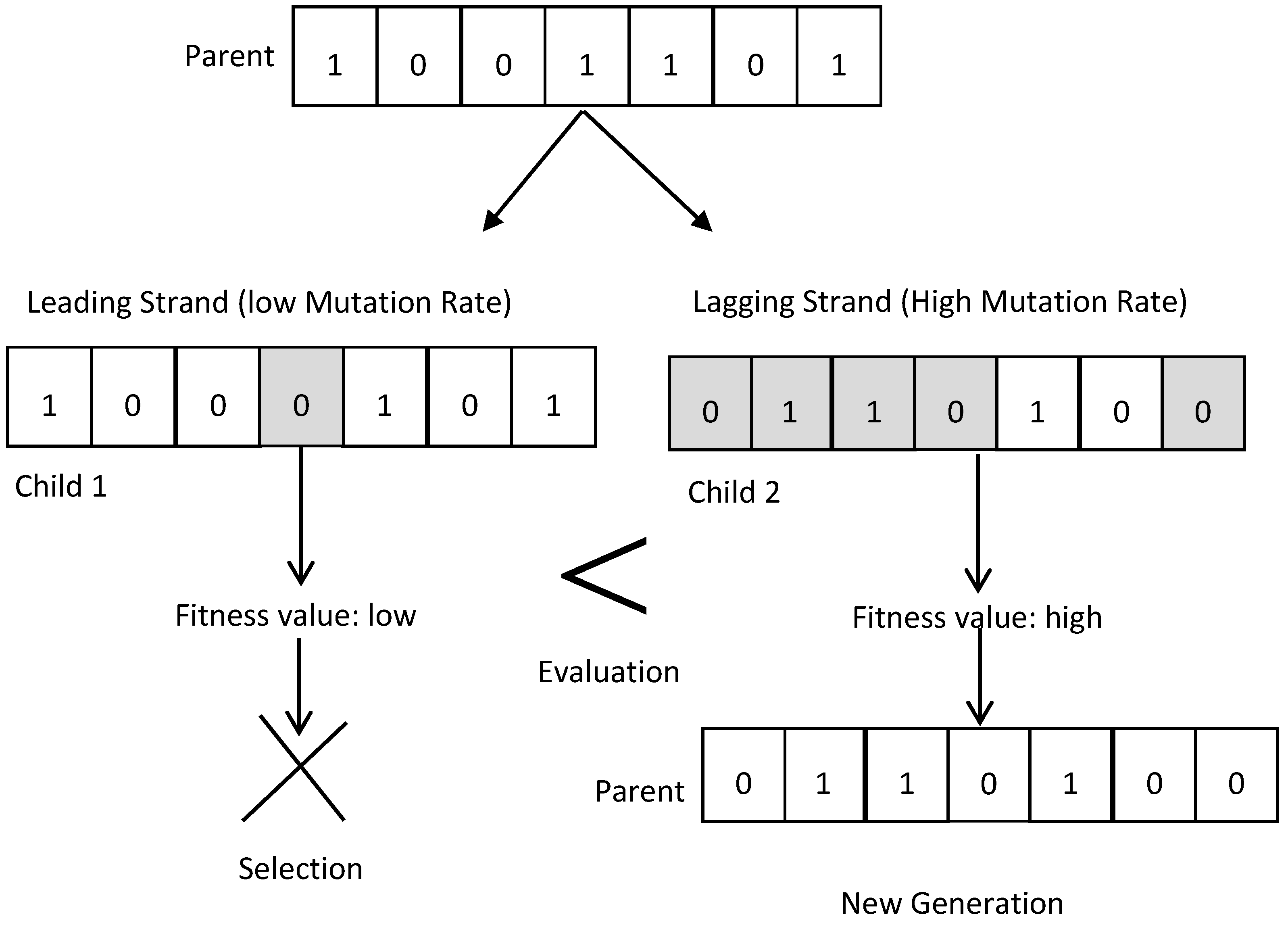
The DEGA uses PIS to simulate evolution. Under the survival rule, it calculates the fitness for each of the individual populations, which is randomly created. In DEGA, the individual inside the random population is called a chromosome. Each chromosome is represented by binary numbers {0, 1}, which also represent the generation unit. 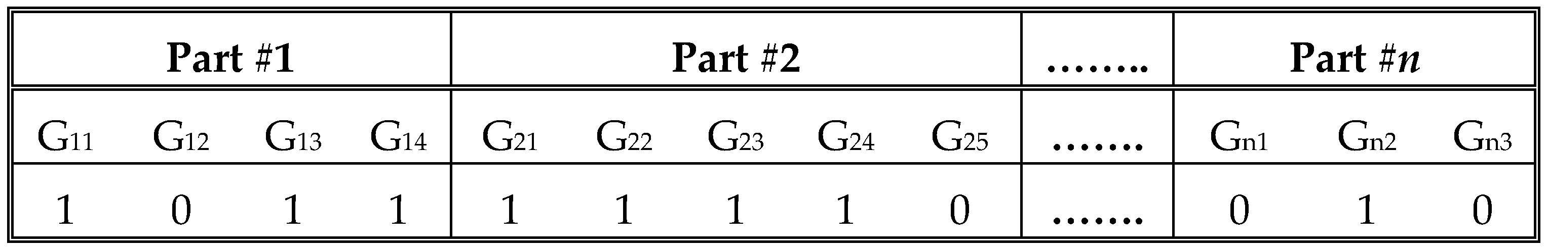During the simulation of the generating system reliability, it is assumed that there are two states, up and down, and the chromosome length “L” refers to the total number of components or generators system. Identical components or generators are split into groups, with each particular group representing a part of a chromosome. Thus, each chromosome will consist of “n” parts. Additionally, each chromosome represents the system states capacities. Figure 4 shows that, each chromosome is represented by a number of components.

In the process of evaluating the adequacy of power generation, the applied elementary model consists of a conventional generating unit model and a chronological load model. These two models are incorporated or superposed to produce the risk model. This study only considers any available generating capacity to represent the risk model in comparison with the expected load of the system.

Hence, by employing the DEGA, each chromosome represents a state in the system. In the space state of the system, the chromosome with a capacity that is higher than the total load represents a success state, while the chromosome with a capacity that is lower than the total load represents a failure state. In order to construct the system state array to estimate the generating system adequacy, this study considers chromosomes in the failure state during a search in the state space pruning of the system.

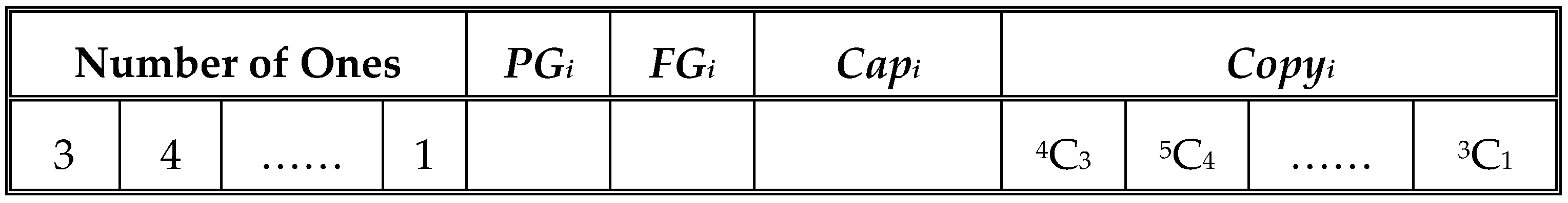
State array chromosomes are responsible for the highest contribution to the loss states in a load, which, therefore, consists of the binary data of the chromosomes after performing the evaluation process when selecting from random initial populations to be a store. The state array consists of fields that represent the information evaluated from the chromosomes. Such information is stored in these states array groupings. The first field has an array with several columns similar to the number of chromosome parts. The column includes several generators in the upstate mean (take bit one) in a similar part. In the remaining fields of state array area range, each of this state “i” contains generation capacity (Cap_i), probability (PG_i), the total number of equivalent permutations (Copy_i) and frequency (FG_i). 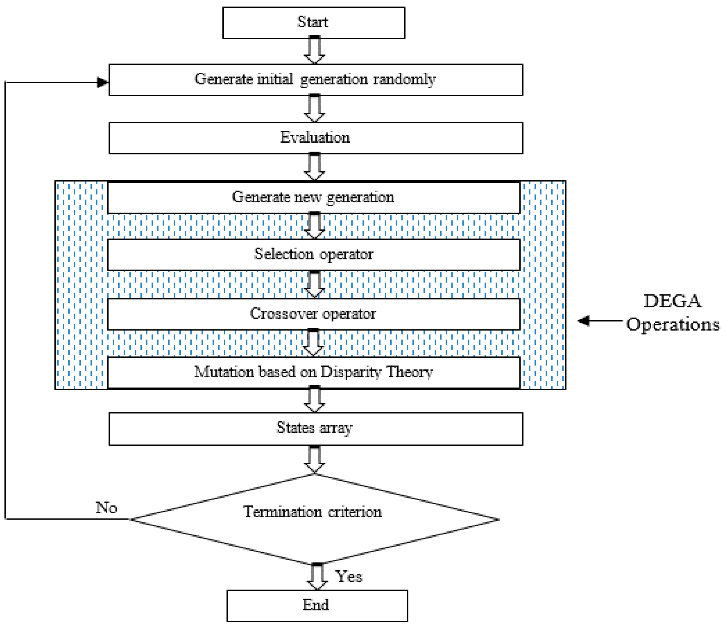Figure 5 depicts the construct of the state array which displays the chromosome stored in these fields.

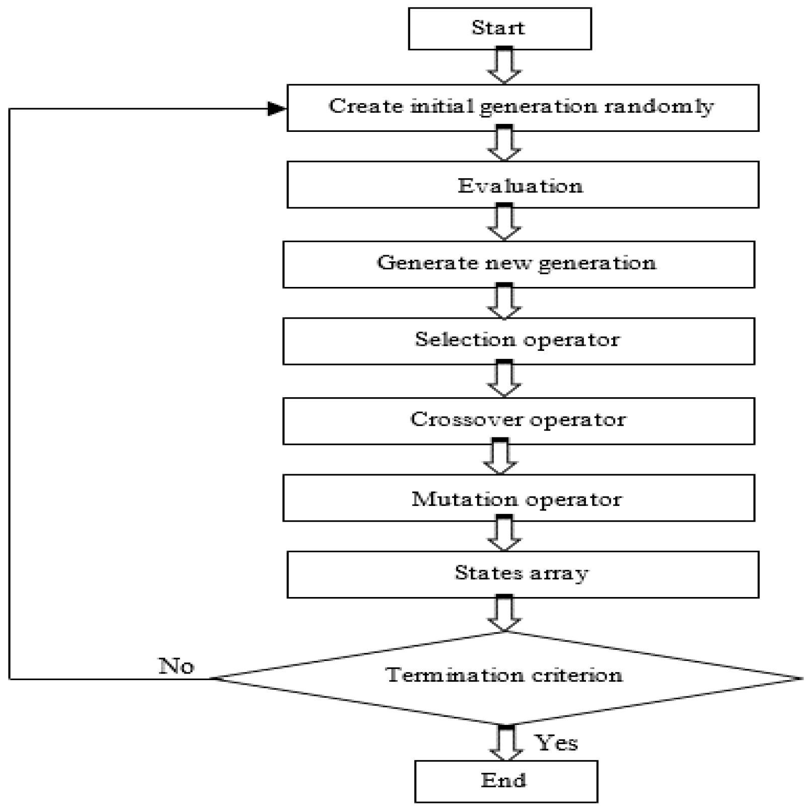
To evaluate the adequacy of the generating system, the initial procedure is in construct the array of failure-states with regards to the total load demand using DEGA. The next step is the indices for reliability, which is calculated through the convolution of the effective available capacity, where the chronological load is based on the state array previously achieved. The constructions of the state array are summarized as follows:

Step 1: The values of the control parameters of the DEGA is set, which include pop_size, P_c, and P_m, which has a double structure. Then, values are set, which include the probability of the leading strand (P_le), and of the lagging strand (P_la), and the reliability parameters (FOR, µ, λ) for the generation unit and threshold probability (t_p).

Step 2: Each chromosome is arranged in “n” parts; each part includes adjacent binary number representation for the conventional generating units, with the same reliability parameters and MW capacity.

Step 3: The length of the chromosome, when part number i is represented as L_i:

$$m={\displaystyle \sum }_{i=1}^n{L}_i$$

(4)

Step 4: Therefore, each chromosome represents the system state capacity.

Step 5: The initial population is randomly generated, with each bit having a random binary number [0, 1]; this procedure is repeated for all initial populations of the chromosomes.

Step 6: The state array that must be saved is constructed.

Step 7: The effective generating capacity of system state i; is calculated:

$$Ca{p}_i={\displaystyle \sum }_{j=1}^{m_g}{b}_j·g_j$$

(5)

where b_j represents the state of the generating unit j; m_g refers to the number of generating units; g_j refers to the MW capacity of each unit. If the capacity Cap_i > L_mxa, it represents the chromosome state of success, therefore, the fitness of its corresponding chromosome is allocated a very small value so as to reduce its chance to influence the next generation population.

Step 8: The failure state of the system state “i” is calculated; if Cap_i < L_mxa, then the state is in the failure state. Therefore, the chromosome failure probability is calculated as follows:

$$P_i={\displaystyle \prod }_{j=1}^{m_g}{P}_j$$

(6)

where m_g is the number of generating unit j; P_j is the probability value, which can take one of these two values: if b_j = 1, then P_j = 1 − FOR_j, and if b_j = 0, then P_j = FOR_j.

The number of all the possible permutations for the evaluated state i is identified as follows:

$$Cop{y}_i=\left(\begin{array}{c}{L}_1\\ O_1\end{array}\right)x,\dots x\left(\begin{array}{c}{L}_j\\ O_j\end{array}\right) ,\dots ,x\left(\begin{array}{c}{L}_n\\ O_n\end{array}\right)$$

where O_j refers to the number of “noes” in group j of length L_n.

Equation (7) is used to calculate the fitness of the system state:

$$Fi{t}_i=Cop{y}_i · P_i or Fi{t}_i=P_i$$

(7)

The objective function is applied in this algorithm and maximized by the DEGA based optimizer search.

The frequency is determined according to the method described by [16]. In this study, the system state is determined by:

$$F{G}_i=P_i ·\left({\displaystyle \sum }_{j=1}^m(1-b_j)·{\mu }_j-{{\displaystyle \sum }}_{j=1}^m{b}_j·{\lambda }_j\right)$$

(8)

where b_j refers to the generating unit state; while µ_j, and, λ_j indicate the respective rates for repair and failure of the generating unit j.

Step 9: The information on eligible chromosome state is saved.

The above process is repeated for all the chromosomes until all the remaining states are evaluated. All chromosomes are checked before being evaluated to ensure that they are not previously saved from another evaluation step. If the state has been saved previously, a very small number of the fitness is assigned so that the probability of this state could be multiplied to reduce the chance of it appearing in the next generation. This state is disregarded and is not added to the state array.

Step 10: The number of iterations is increased by one.

Step 11: Each stopping criterion is checked to determine whether it is met, so that the algorithm could be paused, and the output of the state array can be derived. If the stopping criterion is not met, step 12 will be conducted.

Step 12: Different DEGA operators are adopted to produce the next generation, then, Steps 6 to 9 are repeated until all stopping criteria are met.

Step 13: The reliability indices were calculated based on the previously achieved state arrays.

3.3. Calculating Reliability Indices

Any of the stopping criteria mentioned in [16] could be used to stop the DEGA. The reliability indices for LOLE, LOEE, and LOLF are calculated based on the achieved state arrays and the convolution of the hourly load values. This study considers the L_i, to represent the discrete values for the load levels at the hour (t). The loss of load probability (LOLP) load value is evaluated as shown:

$$\mathrm{LOLP}(L{H}_i)={\displaystyle \sum }_{j=1}^{\mathrm{sa}}{S}_j·P_j·Cop{y}_j$$

(9)

where sa represents the total number of state arrays, while, the status of the system state is S_j. The status value will be equal zero if it is a success state, i.e., Cap_j ≥ LH_i, while the status value is equal to one if it is a failure state, i.e., Cap_j < LH_i. After the LOLP is done for all load levels, the LOLE per year in an hour is measured using Equation (10):

$$\mathrm{LOLE}={\displaystyle \sum }_{j=1}^{8736}\mathrm{LOLP}(L{H}_j)$$

(10)

The expected power not supplied (PNS) in each load level per hour (in megawatts) is calculated using the following Equation (11):

$$PNS(L{H}_i)={\displaystyle \sum }_{j=1}^{sa}{S}_j P_j·Cop{y}_j·(L{H}_i-Ca{p}_j)$$

(11)

$$\mathrm{LOEE}={\displaystyle \sum }_{j=1}^{8736}PNS(L{H}_j)$$

(12)

The calculation for LOLF involves two main components; frequency due to load fluctuation FL, and frequency of generating system capacity FG [11]. Each component is calculated independently, as follows:

$$\mathrm{LOLF}(L{H}_i)={\displaystyle \sum }_{j=1}^{sa}{S}_j·F{G}_j·Cop{y}_j$$

(13)

$$FG={\displaystyle \sum }_{j=1}^{8736}\mathrm{LOLF}(L{H}_j)$$

(14)

$$FL={\displaystyle \sum }_{j=2}^{8736}{V}_j·[\mathrm{LOLP}(L{H}_j)-\mathrm{LOLP}(L{H}_{j-1})]$$

(15)

The V_j equals “zero” when negative value represents the value between the brackets and is equal to “one” otherwise. Meanwhile, the indices for annual LOLF occurrences can be calculated using Equation (3).

This algorithm has several advantages, such as in the construct of the probability outage capacity table of the generating system. It can also determine how much the combinations of the generating unit contribute to the failure state of the system. This is useful in increasing these units’ reliability or when there is an attempt to add more units into the system.

4. Results and Discussion

The IEEE-RTS-79 and RTS-96 were developed to fulfill the need for a standardized database that can test and compare results between proposed algorithms for the reliability assessment of the generating system. The simulation is implemented using a PC computer with the following specifications: Intel(R) Core (TM) i7, CPU 2.40 Hz, and 16 GB RAM. The algorithm was run by using MATLAB R2015b.

4.1. Case (1): IEEE RTS-79

The IEEE Reliability Test System-79 [21], was chosen as the test to examine the proposed DEGA. The IEEE-RTS-79 consisted of 32 generation units, with unit capacities ranging from 12 MW to 400 MW. In the meantime, the system had total power output of 3405 MW, and the peak load of 2850 MW.

To select parameters for DEGA the following steps should be considered. For a certain system, it is suggested to begin by choosing any set of parameters. In this particular simulation, constant mutation rate was utilized in both the leading and lagging strand. The range of P_c should be from 0.1 to 0.9 and the initial population size is required to be higher when compared to the total number of components of the system or generation units [16]. As the system size increases, the threshold probability (t_p) is expected to decrease. Parameter running is required to be carried out just once on a particular system, depending on size.

The recorded value settings of the control parameters for the DEGA, were taken as follows: pop_size = 40, P_c = 0.6. P_m in this regard, there were two components, which were set according to the following values; P_le = 0.06; and P_la = 0.6, while the reliability parameters (FOR, µ, λ) for generation unit settings followed the data reported in [22], and t_p = 1 × 10⁻¹⁵. The load model, load duration curve, was used to generate hourly values, which gave (8736) individual values for the given year. The DEGA was stopped after producing 750 individual generations. Consequently, the overall number of elements that had been saved in the state array was 11,487 states, while the overall permutation number was 3.034497 × 10⁸, compared with the results given in [23], whereas state array was 10,428 states and permutation number was 1.91983 × 10⁷. The DEGA has many advantages over the MSGA through the accelerated evolution velocity, through the application of the variety into the probability of mutation (P_m). The previous work in [23] used a GA with the initial pop_size of 40, P_m = 0.06, and was run for 750 generations. In comparison DEGA has a pop_size of 40, P_le = 0.06; P_la = 0.6, and was run for 750 generations. Subsequently, these 750 generations will be able to generate the totality of the state’s array. Thus, the number of state arrays that was created by this algorithm was larger than the state array obtained by the MSGA. Meanwhile, the same cut-off threshold value was used.

These DEGA results obtained were compared with results obtained from algorithms reported in [16,21,24], as listed in

Table 1. DEGA results for IEEE-RTS-79.

Reliability Indices	Monte Carlo [21]	Unit Addition Algorithm [24]	MSGA [16]	DEGA
LOLE (h/year)	9.371	9.355	9.324	9.360
LOLE Error (%)	0.24%	0.42%	0.74%	0.36%
LOEE (MWh/year)	1197	1168	1163	1183
LOEE Error (%)	−1.78%	0.68%	1.1%	−0.59%
LOLF (occ/year)	1.919	2.019	2.003	2.400
LOLF Error (%)	0%	−5.21%	−4.37%	−25.06%

. The results represent the comparison in reliability indices between three algorithms from the literature. The absolute values of this comparison came from a single run of the DEGA, and of the MSGA to obtain the exact results. The DEGA was stopped after producing 100 individual generations.

To confirm the strength and confidence of the DEGA, a series of 100 runs of the algorithm have been made in the same conditions as previously discussed, and the results are listed in

Table 2. Results of 100 repeated runs of DEGA.

Reliability Indices	Analysis Method [25]	DEGA (Mean)	Error (%)
LOLE (h/year)	9.394	9.384	0.10%
LOEE (MWh/year)	1176	1122	4.59%
LOLF (occ/year) [21]	1.919	1.856	3.28%

. The results from DEGA are compared with results reported in [25].

The computational burden for the proposed method is evaluated against the MCS, unit addition, and MSGA algorithms as listed in

Table 3. Computational time comparison between unit addition, MSGA, and MCS method.

Techniques	Monte Carlo [21]	Unit Addition [24]	MSGA [16]	DEGA
			No. of Generations = 750	No. of Generations = 100
LOLE (h/year)	9.541	9.355	9.324	9.360
time (s)	372	50	177	9

. The computational effort for the proposed method is compared with unit addition and MSGA algorithms, and depends upon the desired accuracy. Meanwhile, the comparison with MCS based on the simulation is stopped when the coefficient of variation reaches 5% [21]. As can be seen from Table 3, the DEGA computational time is faster than the other methods.

Another form of data that can be gathered from state array, is the table for the generating outage capacity. Consequently, this method is advantageous as the outage capacity table obtained is near to the precise outage capacity, and does not have any round-off. Furthermore, one can construct a table based on the state array by putting the states in ascending order based on their capacities. In this regard, the state arrays from the DEGA were sequenced based on the probabilities for their total failure, as listed in

Table 4. State array from the DEGA for IEEE-RTS-79.

No. of Ones									Total Prob.	Capacity (MW)	Copy
Part 1	Part 2	Part 3	Part 4	Part 5	Part 6	Part 7	Part 8	Part 9
4	3	6	4	3	3	3	0	1	0.00012837	2468	160
5	4	5	4	3	3	3	0	1	0.00068744	2450	48
5	4	6	3	2	4	3	0	1	0.00076037	2479	24
5	3	5	4	3	4	3	0	1	0.00173031	2585	48
4	4	6	4	3	4	3	0	1	0.00361543	2643	10
5	4	5	4	3	4	3	0	1	0.01006852	2605	12
5	4	6	4	2	4	3	0	1	0.01127081	2555	6
5	4	5	4	3	4	3	1	0	0.01451494	2555	12

.

Moreover, the DEGA has the ability to construct a state array that is neutral of the system load curve. Thus, only the maximum values from the load curve maximum value set are required if we need to calculate the reliability for varied load curves for the system configuration. DEGA can utilize these values to find out the state array in the system state space. Moreover, as shown by the state array obtained, it has become apparent how each system state contributes to the total system adequacy, and the capacity outage table can also be built from it. Furthermore, as long as the actual peak load is not larger than the one used for deriving the state array, the state array achieved can always be used to calculate the actual adequacy indices for various scenarios with different peak loads.

Table 5. DEGA results offer a LOLE hours per year comparison.

Max. Load (MW)	2750 MW	2850 MW	2950 MW	3050 MW
Monte Carlo	4.85	9.37	17.369	30.717
Unit addition algorithm	4.84	9.35	17.499	31.031
MSGA	4.82	9.34	17.461	31.017
DEGA	4.71	9.36	17.330	30.800

,

Table 6. The DEGA results offer a LOEE per year comparison.

Max. Load (MW)	2750 MW	2850 MW	2950 MW	3050 MW
Monte Carlo	586.49	1197.44	2335.73	4385.69
Unit addition algorithm	561.80	1168.00	2311.50	4379.90
MSGA	558.58	1165.89	2310.10	4383.72
DEGA	529.32	1186.00	2579.69	4314.26

and

Table 7. The DEGA results offer a LOEF occurrences per year comparison.

Max. Load (MW)	2750 MW	2850 MW	2950 MW	3050 MW
Monte Carlo	1.034	1.919	3.422	5.865
Unit addition algorithm	1.084	2.019	3.634	6.191
MSGA	1.076	2.009	3.624	6.190
DEGA	1.030	1.920	3.390	5.460

show a comparison of the results obtained for different load curves using the MCS [21], unit addition algorithm [24], the MSGA [16], and the DEGA method. The state array in this study was constructed using the maximum load of 3050 MW. It was then superposed with the four different load curves. It can be seen from Table 5, Table 6 and Table 7 that the DEGA has given acceptable results compared to the previous algorithm, which was mentioned earlier.

4.2. Case (2): IEEE RTS-96

Since the RTS-79 system was published it has become useful in assessing different reliability modeling and evaluation methodologies for several types of research. Additionally, since then, few modifications have been made in the electric utility industry and this implies a multi-area RTS can be designed by integrating additional data. The configuration of the IEEE-RTS-96 was updated from a version of the original RTS-79. Therefore, it is designed to consist of three areas from RTS-79, which are connected together by transmission lines. The IEEE Reliability Test System-96 [26] was also chosen to test the proposed DEGA. The IEEE-RTS-96, consisting of 96 generation units, used unit capacities that ranged from 12 MW to 400 MW. The total power output of the system was 10,215 MW, and the system had a peak load of 9000 MW. The values of the control parameters for the DEGA were set as follows: pop_size = 100, P_c = 0.6; P_le = 0.01; P_la = 0.4. The reliability parameters (FOR, µ, λ) for generation unit settings followed the data of [24], and t_p = 1 × 10⁻²⁰. The load duration curve was used to generate hourly individual values for the given year. The DEGA was stopped after producing 350 individual generations. The results obtained from DEGA were compared with the results obtained from the algorithm in [14], as listed in

Table 8. DEGA results for IEEE-RTS-96.

Reliability Indices	MSGA	DEGA	Percentage Error
LOLE (h/year)	1.113	1.110	0.26%
LOEE (MWh/year)	220.5	254.2	15.2%

. Furthermore, this Table represents the comparisons in the reliability indices between algorithms represented in absolute values from a single run of the DEGA, and of the MSGA, to obtain the exact results.

5. Conclusions

This paper introduces a novel DEGA, in which the performance of the probability of mutation in an MSGA was improved by incorporating features from a paradigm into disparity theory. Moreover, the DEGA can increase the production of a variety of individuals in an early stage of the next population generation, and it is also an efficient search tool when using the disparity theory of evolution. Test systems, IEEE-RTS-79 and IEEE-RTS-96, were used to demonstrate the effectiveness of the developed algorithm. Furthermore, the simulation steps and the results of the reliability assessment of the generating system were demonstrated, by comparing them with other methods so that the efficiency of the algorithm proposed could be validated. This study has confirmed that the efficiency of selection for the probability of mutation can lead to significant improvements in the population fitness due to the use of the disparity model. Therefore, this technique is promising for the improvement of the GA by increasing and doubling the generated majority of failure states to provide a good approximation of the assessment of reliability indices to be calculated.