Adaptive State Feedback—Theory and Application for Wind Turbine Control

Abstract

A class of adaptive disturbance tracking controllers (ADTCs) is augmented with disturbance and state estimation and adaptive state feedback, in which a controller and estimator, which are designed on the basis of a lower-order model, are used to control a higher-order nonlinear plant. The ADTC requires that the plant be almost strict positive real (ASPR) to ensure stability. In this paper, we show that the ASPR property of a plant is retained with the addition of disturbance and state estimation and state feedback, thereby ensuring the stability of the augmented system. The proposed adaptive controller with augmentation is presented in the context of maximum power extraction from a wind turbine in a low-wind-speed operation region. A simulation and comparative study on the National Renewable Energy Laboratory’s (NREL’s) 5 MW nonlinear wind turbine model with an existing baseline Proportional-Integral-Derivative(PID) controller shows that the proposed controller is more effective than the existing baseline PID controller.

1. Background

Electrical energy generated from wind power is one of the major sources of renewable energy. The size of the wind turbine has to be large in order to reduce the cost of the energy; however, this increase in size comes with the cost of added weights in its structures [1]. For large wind turbines, the blade is one of the most important structures that needs to be considered for both fatigue life and weights. Using stiff materials to construct wind turbine blades increases the blade’s life, but it also increases its weight significantly. This requires a larger foundation and tower to support the blades, which results in high installation costs and an increase in the cost of energy. On the other hand, using lightweight materials reduces the weight significantly, but the blade becomes highly flexible, which makes it prone to damage by different types of aerodynamic and structural loading. Stiffening the blade is not a viable option for a large wind turbine. However, advents in modern control theory have made it possible to reduce the blade loading significantly, thereby making a flexible blade design a viable option [2]. Besides blade loading, other structural loading, such as drivetrain and tower loading, also needs to be considered to increase the life span of the wind turbine, which directly affects the cost of energy. Maximizing the power captured while operating the wind turbine at a below-rated wind speed is another important aspect of a wind turbine control system [3]. Modern wind turbines are capable of operating at variable rotor speeds to accompany the maximum power point tracking algorithm.

A wind turbine is a highly complex dynamical system containing multiple structures connected together. The inclusion of aerodynamics and an aeroelastic interaction with a highly flexible blade makes the system more complex, which introduces uncertainties during modeling. A wide spectrum of controller architecture, such as traditional Proportional-Integral-Derivative (PID) [4], multivariable [5,6], robust [7,8], model predictive [9,10] architecture, and so forth, have been used to achieve different performance goals. However, an adaptive control architecture is very attractive because of its capability to incorporate the uncertainty involved in the system. A class of adaptive controls accompanied with a system identification algorithm has also been successfully used [3]. Intelligent adaptive control strategies have also been used to achieve different control goals for a wind turbine [11,12,13].

A class of adaptive controllers has been developed and studied by Balas [14,15,16], one of the authors of this paper, and was successfully implemented to reject the persistent disturbance on flexible space structures [17] and suppress persistent rotor vibration [18]. Frost and Balas [19] extended this adaptive control theory to control the wind turbine rotor speed in the high-wind-speed region. Another extension of this adaptive control theory, developed by Balas et al., is to maximize the power captured by a wind turbine where the wind speed is assumed to be directly measured [20]. The direct measurement of wind speed is either expensive when LiDAR is used or unreliable when a cup anemometer is used; therefore, we extended this theory to incorporate wind-speed estimation based on the lower-order linear model of wind turbines [21,22]. We demonstrate the effectiveness of this extended control system with wind-speed estimation through controller implementation and simulation on the National Renewable Energy Laboratory’s (NREL’s) 5 MW nonlinear wind turbine model [23]. In this paper, we present the stability analysis of the proposed extension of the adaptive controller. The foundation for the stability of the class of adaptive controllers is presented in [14,24] and it is shown that the system needs to satisfy the almost strict positive real (ASPR) conditions to ensure the stability. We show that the augmentation of state estimation and state feedback still preserves the ASPR properties and hence the stability of the original system.

The rest of the paper is structured as follows. The problem of maximum power point tracking at below-rated wind speeds is formulated in Section 2. Section 3 presents an overview of the wind turbine as a linear time-invariant (LTI) system, introduces the idea of a disturbance generator, and lays out the foundation for partial state estimation with wind-speed estimation. The proposed adaptive control algorithm and the corresponding stability analysis are presented in Section 4; these are followed by the illustration of the proposed controller through the simulation with the 5 MW wind turbine model in Section 5. Section 6 presents the concluding remarks and future research direction for the paper.

2. Problem Formulation

A variable-speed wind turbine has three regions of operation based on the wind speed. Region I is a start-up region, and no power is produced because the wind speed is very low. In Region II, the wind speed is sufficiently high to produce power, and the wind turbine operates at a below-rated speed producing electrical energy. When the wind speed is high enough to produce rated power, the wind turbine operates in Region III. A variable-speed wind turbine is capable of maximizing the power captured while operating in Region II, which is typically achieved by controlling the generator torque.

The power captured by a typical horizontal-axis wind turbine is given by the following [25]:

$$P=\frac{1}{2}\rho A{C}_p{V}^3$$

(1)

where P is the mechanical power captured, A is the rotor disc area, $C_p$ is the power coefficient, $\rho$ is the air density, and V is the free-stream wind velocity.

The power coefficient, which typically represents the fraction of the total wind power converted to mechanical energy in the wind turbine, depends on the tip-speed ratio ($\lambda$) and blade-pitch angle ($\beta$), which can be expressed as follows:

$$\lambda =\frac{\mathsf{\Omega }R}{V}$$

(2)

where $\mathsf{\Omega }$ is the rotor speed and R is the rotor radius.

In the below-rated wind speed region, the wind turbine blades are held at a constant pitch angle; hence the power coefficient is a function of the tip-speed ratio only. The power coefficient initially increases with the increase in the tip-speed ratio and starts decreasing if it is further increased beyond a certain point. Hence, to maximize the power captured by the wind turbine, the power coefficient has to be maximized. This is achieved by operating the wind turbine at a constant tip-speed ratio pertaining to the maximum power coefficient.

To formulate the power maximization problem as the tip-speed-ratio tracking problem, we define the tip-speed-ratio tracking error ($\epsilon$) as the deviation of the current tip-speed ratio from the operating tip-speed ratio as follows:

$$\epsilon =\lambda -{\lambda }_{OP}=\frac{\mathsf{\Omega }R}{V}-\frac{{\mathsf{\Omega }}_{OP}R}{V_{OP}}=\frac{R}{V}\left(\mathsf{\Omega }-\frac{{\mathsf{\Omega }}_{OP}}{V_{OP}}V\right)$$

(3)

where $V_{OP}$ is the operating wind speed in Region II, and ${\mathsf{\Omega }}_{OP}$ is the corresponding operating rotor speed to have the optimum tip-speed-ratio value (${\lambda }_{OP}$). Here we have restated the tip-speed tracking error in some observable quantities, R, $\mathsf{\Omega }$, and V.

Now, assuming both the rotor speed ($\mathsf{\Omega }$) and wind velocity (V) are available, part of Equation (3) can be redefined as the tracking error as follows:

$$e_y=\mathsf{\Omega }-QV$$

(4)

where $Q=\frac{{\mathsf{\Omega }}_{OP}}{V_{OP}}$ is defined as the tracking ratio. Equations (1)–(4) suggest that driving the output tracking error ($e_y$) or tip-speed-ratio tracking error ($\epsilon$) to zero leads to the optimum tip-speed-ratio tracking and hence maximizes the power captured by the wind turbine. To achieve this, a proportional change in the rotor speed is necessary when the wind speed changes, where the constant of proportionality is given by the tracking ratio (Q). To use this formulation, both the wind speed and the rotor speed need to be observed and the rotor speed is changed through the generator torque control scheme.

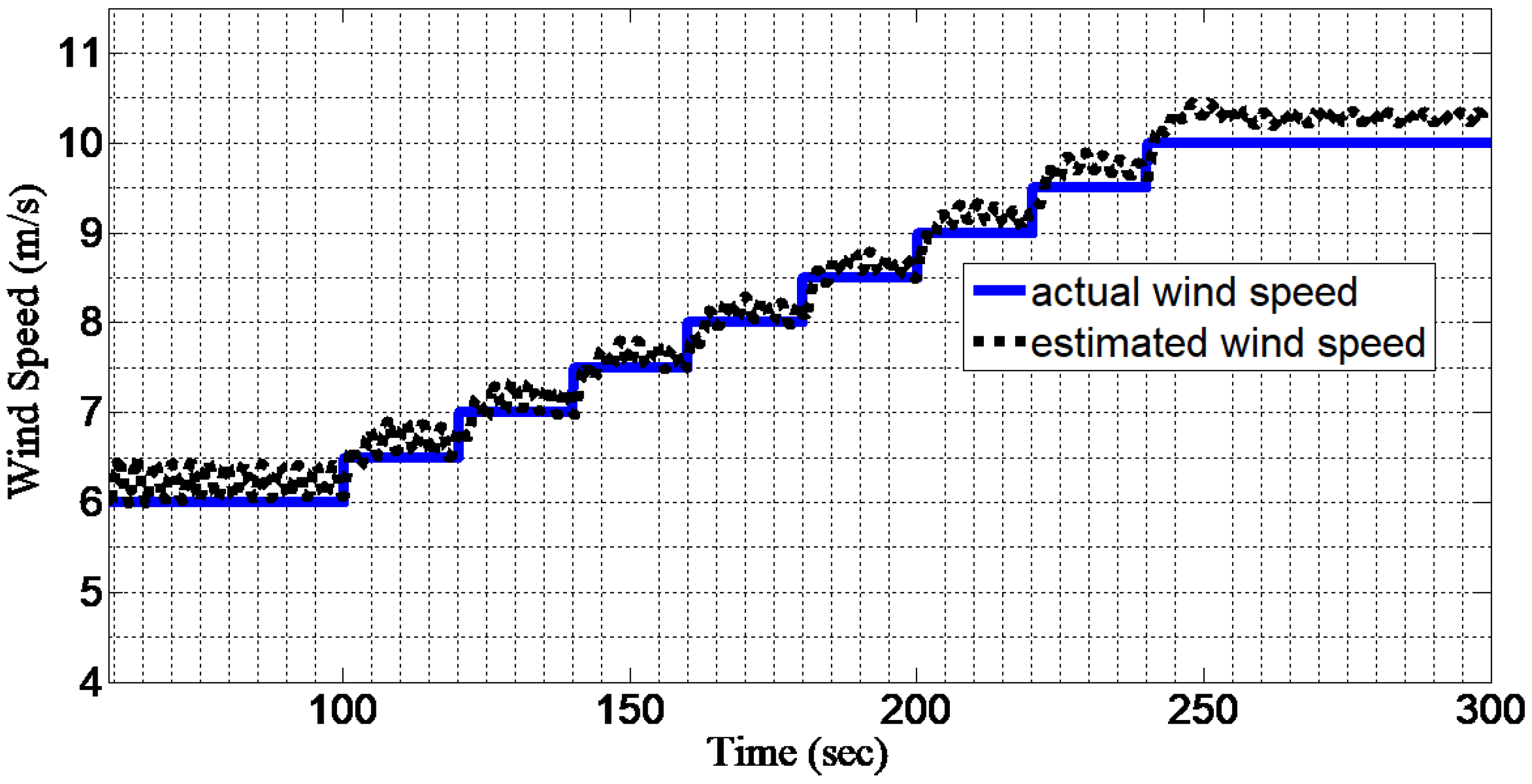
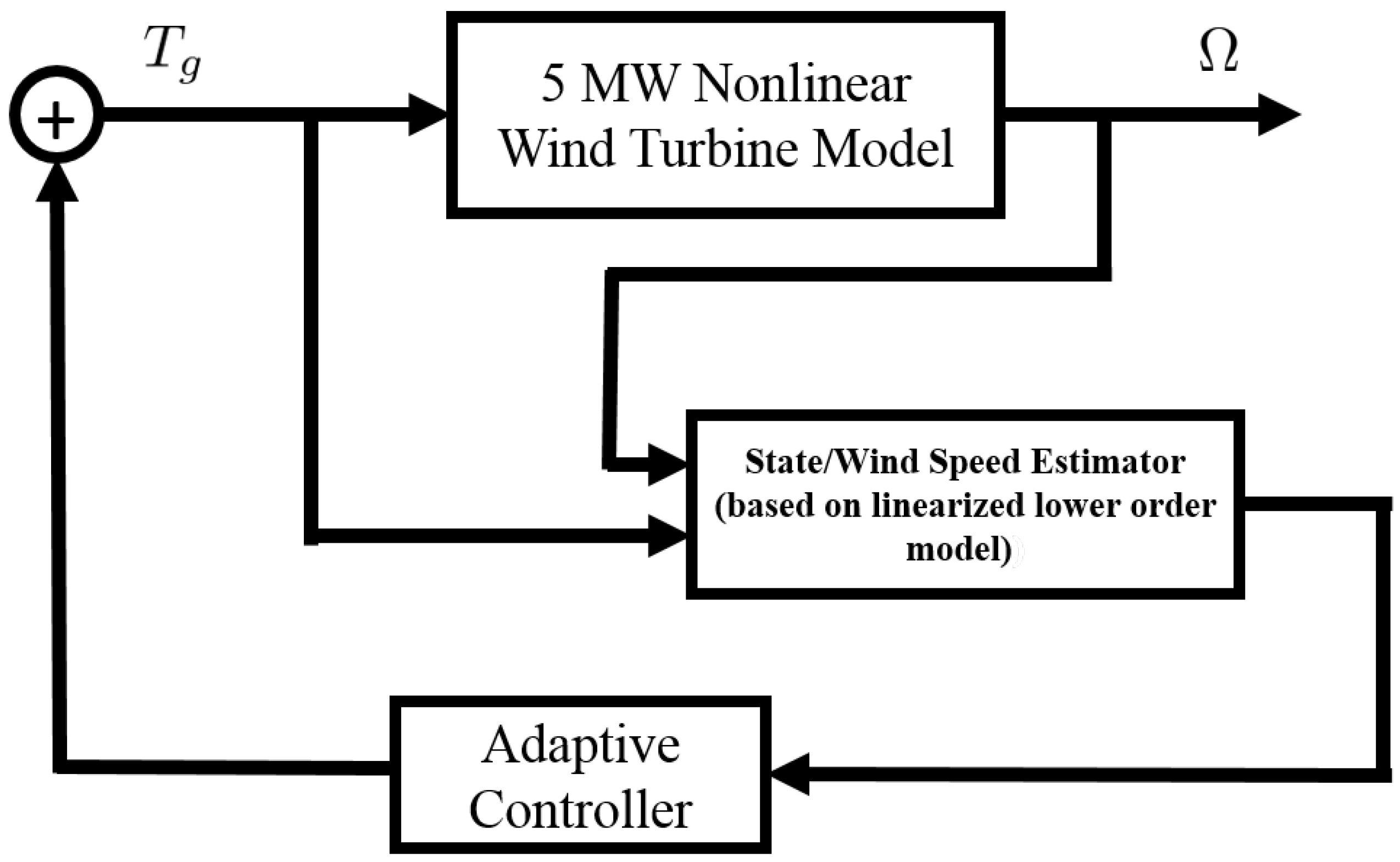
3. System Description and Wind-Speed Estimation

As noted in the previous section, we need to observe both the wind speed and rotor speed to incorporate the output error and tip-speed-ratio tracking error equations (Equations (3) and (4)) in the control system design. A simple rotary encoder would be sufficient to measure the rotor speed. However, the wind speed measurement is not an obvious task. A cup anemometer and LiDAR are the two most extensively used technologies for in situ measurements of wind speed. A cup anemometer lacks the accuracy to be incorporated in the control system loop. LiDAR, on the other hand, is a very expensive solution to measure wind speed accurately. Moreover, LiDAR measures the wind speed well ahead of the wind turbine, and hence its measurement must be accompanied with a wind evolution model to predict the wind speed at the rotor [26]. Therefore, we propose a method to estimate the wind speed from the rotor speed measurement.

We suppose the wind turbine dynamics is modeled as a LTI state-space formulation as follows:

$$\begin{array}{cc}\hfill \dot{x}& =Ax+Bu+\Gamma u_D\hfill \\ \hfill y& =Cx+Du\hfill \end{array}$$

(5)

where x is an N-dimensional state vector, u is a P-dimensional input vector, $u_D$ is a $p_D$-dimensional disturbance input vector, and y is an M-dimensional measurement vector. $A,B,C,D$, and $\Gamma$ are matrices having appropriate dimensions obtained from the physical parameters of the wind turbine. Because the matrix D is zero for most of the practical systems and because this also holds true for the system under study, we do not incorporate this term for simplicity in the analysis; however, the inclusion of this term does not alter the analysis in later sections.

Because we are interested in the control of a higher-order model using a subset of states, a lower-order representation of Equation (5) can be written as follows:

$$\begin{array}{cc}\hfill {\dot{x}}_m& =A_m{x}_m+B_m{u}_m+\Gamma u_D\hfill \\ \hfill y& =C_m{x}_m\hfill \end{array}$$

(6)

Here we assume the same set of measurements for both the full state and lower-order system, therefore representing the output with the same symbol y.

To align this system with the wind-speed tracking problem formulation of the previous section, $u_m$ is taken as a generator torque command, $u_D$ is taken as the wind speed (noting that both $u_D$ and V are used interchangeably to represent the wind speed), and y is taken as the rotor speed (also noting that we use y and $\mathsf{\Omega }$ interchangeably to represent the rotor speed). The state vector ($x_m$) consists of many system response parameters and/or a combination of these as per the control system performance requirement.

Taking reference from [27], we assume that the wind comes from a disturbance generator of the following form:

$$\begin{array}{cc}\hfill u_D& =\Theta z_D\hfill \\ \hfill {\dot{z}}_D& =F{z}_D;z_D\left(0\right)=z_0\hfill \end{array}$$

(7)

where the disturbance or wind speed vector ($u_D$) is assumed to have evolved from disturbance states ($z_D$), and $\Theta$ and F are the appropriate matrices representing a known form of disturbance [17].

Assuming that the form of disturbance is known (e.g., sinusoidal, step, etc.), the disturbance state vector ($z_D$) can be composed from the appropriate basis functions (${\phi }_D$) as follows:

$$z_D=L{\phi }_D$$

(8)

where L is the matrix combining the known basis functions for the disturbance (${\phi }_D$).

For this paper, we assume the wind to be a step disturbance. This assumption is also valid for turbulent disturbance because we can assume the turbulent wind profile to be formed from the combination of steps. Then, the disturbance-state basis function can be taken as ${\phi }_D=1$. Additionally, because a step function consists of a constant value, its derivative will be zero; hence it is imperative to use $F=0$ in Equation (7). Because only the form of disturbance is known, hence we assume that the exact values of L and $\Theta$ are unknown. For a step disturbance generator, we could ideally assume $\Theta =constant$ and use $\Theta =1$ when needed. In conclusion, Equations (7) and (8) represent a disturbance generator model from which the wind speed is assumed to be generated.

To estimate the wind speed, Equations (6) and (7) are combined together to form an augmented model as follows:

$$\begin{array}{cc}\hfill \left[\begin{array}{c}{\dot{x}}_m\\ {\dot{z}}_D\end{array}\right]& =\underset{{\overline{A}}_m}{\underbrace{\left[\begin{array}{cc}{A}_m& \Gamma \Theta \\ 0& F\end{array}\right]}}\underset{z}{\underbrace{\left[\begin{array}{c}{x}_m\\ z_D\end{array}\right]}}+\underset{{\overline{B}}_m}{\underbrace{\left[\begin{array}{c}{B}_m\\ 0\end{array}\right]}}u\hfill \\ \hfill y& =\underset{{\overline{C}}_m}{\underbrace{\left[\begin{array}{cc}{C}_m& 0\end{array}\right]}}\hfill \end{array}$$

(9)

Typically the pair (${\overline{A}}_m,{\overline{C}}_m$) is observable and an appropriate state estimator can be designed on the basis of Equation (9) as follows:

$$\begin{array}{cc}\hfill \dot{\widehat{z}}& ={\overline{A}}_m\widehat{z}+{\overline{B}}_{m}u+\overline{K}(y-\widehat{y})\hfill \\ \hfill \widehat{y}& ={\overline{C}}_m\widehat{z}\hfill \end{array}$$

(10)

where ($\widehat{.}$) represents the estimated quantities.

The estimated state vector ($\widehat{z}$) in Equation (10) consists of both lower-order wind turbine states (${\widehat{x}}_m$) and the states corresponding to the wind speed (${\widehat{z}}_D$). Therefore, this equation provides an estimation of the wind speed along with the desired plant states. In particular, the estimated wind speed can be obtained from the disturbance generator of Equation (7) as follows:

$${\widehat{u}}_D=\Theta {\widehat{z}}_D$$

(11)

We note that the measured variable (y) is the rotor speed ($\mathsf{\Omega }$) for this particular case.

The output tracking error of Equation (4) can now be updated according to the estimated wind speed as follows:

$${\widehat{e}}_y=\mathsf{\Omega }-Q{\widehat{u}}_D$$

(12)

where $u_D$ in Equation (4) is replaced with the estimated wind speed (${\widehat{u}}_D$). Then the control objective is to drive the estimated output error (${\widehat{e}}_y$) to zero by controlling the measured rotor speed ($\mathsf{\Omega }$ or y) through a torque controller.

4. Adaptive Controller

To drive the estimated output tracking error of Equation (12) to zero, we use an adaptive controller of the following form:

$$u=G_e{\widehat{e}}_y+G_x{\widehat{x}}_m+G_D{\phi }_D$$

(13)

with the gain adaption laws:

$$\begin{array}{cc}\hfill {\dot{G}}_e& =-{\widehat{e}}_y{\widehat{e}}_y^T{\gamma }_e;{\gamma }_e>0\hfill \\ \hfill {\dot{G}}_D& =-{\widehat{e}}_y{\varphi }_D^T{\gamma }_D;{\gamma }_D>0\hfill \\ \hfill {\dot{G}}_x& =-{\widehat{e}}_y{x}_m^T{\gamma }_x;{\gamma }_{x_m}>0\hfill \end{array}$$

(14)

where $G_e$, $G_D$, and $G_x$ are the adaptive gains with corresponding gain adaption laws from Equation (14), and ${\gamma }_D,{\gamma }_e,$ and ${\gamma }_x$ are the arbitrary positive definite matrices that should be tuned to obtain the desired performance.

Equation (14) presents only the statement of gain adaption laws, and details of these gain adaption laws can be found in [14]. The focus of this paper is to prove that the proposed adaptive laws and the corresponding gain adaption laws are stable under certain conditions.

Closed-Loop System Formulation

In this section we formulate the dynamics of a closed-loop system on the basis of the wind turbine dynamics represented by Equations (5) and (6) that incorporates the adaptive control law of Equation (13) with the adaptive gains of Equation (14). We begin with the sufficient condition for the stability and convergence of the closed-loop system incorporating the proposed adaptive controller that does not have adaptive state feedback. We only state the conditions here, and the necessary proof can be found in [28].

Theorem 1.

A system represented by state-space matrices ($A,B,C,D$) will be stable under the adaptive feedback control given by Equations (13) and (14) (without adaptive state feedback term $G_x{\widehat{x}}_m$ or corresponding gain adaption term ${\dot{G}}_x=-{\widehat{e}}_y{x}_m^T{\gamma }_x$) if ${\phi }_D$ is bounded and the system is ASPR. A system is ASPR if

• it is non-minimum-phase;
• the product $CB$ of system matrices is positive (or $CB>0$).

(We refer to [24] for a detailed discussion.)

Because Theorem 1 in [28] does not incorporate the adaptive state feedback term, it is imperative to prove that the stability of the system is preserved with augmentation of adaptive state feedback. For this, we form a closed-loop system for the system under study and show that the corresponding pseudo-open-loop system (this will be clear later) preserves the ASPR properties.

The state estimation Equation (10) can be re-stated as follows:

$$\begin{array}{c}\hfill \dot{\widehat{z}}=L_{21}y+L_{22}\widehat{z}+L_{23}u\end{array}$$

(15)

where each variable y, $\widehat{z}$, and u in Equation (10) is separated, and $L_{21},$$L_{22}$, and $L_{23}$ represent the corresponding matrices from Equation (10).

To have a more general formulation, we assume that the lower-order augmented state vector (z) is obtained from a linear transformation of the full-order state vector augmented with a disturbance generator, or $z=Tw\ni w\equiv {\left[x{u}_D\right]}^T$. Then, the estimation error can be expressed as follows:

$$\begin{array}{ccc}& \hfill e& =\widehat{z}-z=\widehat{z}-Tw\hfill \\ \hfill \Rightarrow & \hfill \widehat{z}& =Tw+e\hfill \end{array}$$

(16)

and the dynamics of the full-order state model represented by Equation (9) augmented with the disturbance generator model of Equation (7) can be presented as follows:

$$\begin{array}{cc}\hfill \dot{w}& =\underset{\overline{A}}{\underbrace{\left[\begin{array}{cc}A& \Gamma \Theta \\ 0& F\end{array}\right]}}w+\underset{\overline{B}}{\underbrace{\left[\begin{array}{c}B\\ 0\end{array}\right]}}u\hfill \\ \hfill y& =\underset{\overline{C}}{\underbrace{\left[\begin{array}{cc}C& 0\end{array}\right]}}w\hfill \end{array}$$

(17)

The output tracking error of Equation (4) can also be expressed in terms of the full-order augmented state vector w as follows:

$$\begin{array}{cc}\hfill e_y& =y-Q{u}_D\hfill \\ & =Cx-Q\Theta z_D\hfill \\ & =\underset{{\overline{C}}_e}{\underbrace{\left[\begin{array}{cc}C& -Q\Theta \end{array}\right]}}w\hfill \end{array}$$

(18)

where $w={\left[x{u}_D\right]}^T$ is the full-order augmented state vector.

Now, we define an ideal trajectory for the system to achieve the desired control goal as follows:

$$\begin{array}{cc}\hfill {\dot{w}}_{*}& =\overline{A}{w}_{*}+\overline{B}{u}_{*}\hfill \\ \hfill y_{*}& =\overline{C}{w}_{*}\hfill \\ \hfill e_y^{*}& ={\overline{C}}_e{w}_{*}=0\hfill \end{array}$$

(19)

In Equation (19), $e_y^{*}$ is assumed to be zero, because it is the ideal tracking error and the ideal control objective is to make this zero.

Assuming the existence of a liner transformation $S_1$ that takes a disturbance state vector ($z_D$) to a plant state vector (x), the augmented state (z) can then be expressed as follows:

$$w_{*}=\left[\begin{array}{c}{x}_{*}\\ z_D\end{array}\right]=\underset{{\overline{S}}_1}{\underbrace{\left[\begin{array}{c}{S}_1\\ I_D\end{array}\right]}}{z}_D\equiv {\overline{S}}_1{z}_D$$

(20)

where $I_D$ is the identity matrix of appropriate dimension.

The ideal control input, which results in the desired ideal trajectory, can then be expressed as follows:

$$\begin{array}{c}\hfill u_{*}=S_2{z}_D+G_z^{*}{z}_{*}\end{array}$$

(21)

Now the perturbation of the true system from the ideal trajectory is expressed as follows:

$$\begin{array}{cc}\hfill \Delta w& =w-w_{*}\hfill \\ \hfill \Delta u& =u-u_{*}\hfill \\ \hfill \Delta y& =y-y_{*}\hfill \\ \hfill \Delta e_y& =e_y-e_y^{*}=e_y(\because e_y^{*}=0\mathrm{From}\mathrm{Equation}(19\left)\right)\hfill \end{array}$$

(22)

The dynamics of the perturbation Equation (22) can be expressed as follows:

$$\begin{array}{cc}\hfill \Delta \dot{w}& =\overline{A}\Delta w+\overline{B}\Delta u\hfill \\ \hfill \Delta y& =\left[C0\right]\Delta w\hfill \\ \hfill e_y& =\Delta e_y={\overline{C}}_e\Delta w\hfill \end{array}$$

(23)

Thus, the estimated output tracking can be expressed in terms of the perturbed state vector ($\Delta w$) and augmented state estimation error (Equation (16)) as follows (see Proof 1 in Appendix A):

$${\widehat{e}}_y={\overline{C}}_e\Delta w-Q\Theta H_{D}e$$

(24)

where $H_D=\left[0I_D\right]$.

Noting that the adaptive control law from Equation (13) is $u=G_e{\widehat{e}}_y+G_D{\phi }_D+G_z\widehat{z}$ and assuming the deviation in the control gain ($\Delta G=G-G^{*}$ with $G=\left[G_e{G}_D{G}_z\right]$) as the difference between the true and the ideal gain, the input deviation equation can be expressed as follows (see Proof 2 in Appendix A):

$$\begin{array}{c}\hfill \Delta u=(G_e^{*}\overline{C}+G{z}^{*}T)\Delta w+(G{z}^{*}-G_e^{*}Q\Theta H_D)e+h\end{array}$$

(25)

where $h\equiv [\Delta G_e\Delta G_D\Delta G_z]{\left[{\widehat{e}}_y{\phi }_D\widehat{z}\right]}^T$.

Using this control input in the dynamic equation represented by Equation (23), we obtain the following (see Proof 3 in Appendix A):

$$\begin{array}{cc}\hfill \Delta \dot{w}& =[\overline{A}+\overline{B}(G_e^{*}\overline{C}+G_z^{*}T)]\Delta w+\overline{B}(G_z^{*}-G_e^{*}Q\Theta H_d)e+\overline{B}h\hfill \end{array}$$

(26)

The estimation error dynamics can be expressed as follows (see Proof 4 on Appendix A):

$$\begin{array}{c}\hfill \dot{e}=\dot{\widehat{z}}-z=L_{22}e\end{array}$$

(27)

Now combining the feedback dynamic Equation (26) and error dynamic Equation (27), we can give a closed-loop system as follows:

$$\begin{array}{cc}\hfill \left[\begin{array}{c}\Delta \dot{w}\\ \dot{e}\end{array}\right]& =\underset{{\tilde{A}}_c}{\underbrace{\left[\begin{array}{cc}\overline{A}+\overline{B}(G_e^{*}\overline{C}+G_z^{*}T)& \overline{B}(G_z^{*}-G_e^{*}Q\Theta H_d)\\ 0& L_{22}\end{array}\right]}}\left[\begin{array}{c}\Delta w\\ e\end{array}\right]+\underset{\tilde{B}}{\underbrace{\left[\begin{array}{c}\overline{B}\\ 0\end{array}\right]}}h\hfill \\ \hfill {\widehat{e}}_y& =\underset{\tilde{C}}{\underbrace{[\overline{C}-Q\Theta H_d]}}\left[\begin{array}{c}\Delta w\\ e\end{array}\right]\hfill \end{array}$$

(28)

Now, the closed-loop matrix ${\tilde{A}}_c$ can be decomposed into a pseudo-open-loop system as follows:

$$\begin{array}{c}\hfill {\tilde{A}}_c=\underset{\tilde{A}}{\underbrace{\left[\begin{array}{cc}\overline{A}+\overline{B}{G}_e^{*}T& \overline{B}{G}_z^{*}\\ 0& L_{22}\end{array}\right]}}+\underset{\tilde{B}}{\underbrace{\left[\begin{array}{c}\overline{B}\\ 0\end{array}\right]}}{G}_e^{*}\underset{\tilde{C}}{\underbrace{[\overline{C}-Q\Theta H_d]}}\end{array}$$

(29)

In other words, the closed-loop matrix ${\tilde{A}}_c$ can be viewed as being stemmed from a pseudo-open-loop system represented by ($\tilde{A}$, $\tilde{B}$, $\tilde{C}$) with an output feedback through a feedback gain of $G_e^{*}$. We note that this is just an analogy for the convenience in a closed-loop system analysis.

Now we give three lemmas to prove that the pseudo-open-loop system of Equation (29) is ASPR (see Proof in Appendix A), which will allow us to apply Theorem 1 to prove the stability of the closed-loop system given by Equation (28).

Lemma 1.

The system matrices product ($CB$) of the pseudo-open-loop system is equal to that of the true system or $\tilde{C}\tilde{B}=CB$.

Lemma 2.

The transfer function of the pseudo-open-loop system can be expressed as follows:

$$\tilde{P}\left(s\right)=C{[sI-(A+B{G}_z^{*}{T}_1)]}^{-1}B$$

This system is equivalent to state feedback via a feedback gain of $G_z^{*}$.

Lemma 3.

The state feedback (in the form of Lemma 2) does not alter the minimum phase of a transfer function; or, if the system transfer function $P\left(s\right)=C{(sI-A)}^{-1}B$ is minimum-phase, then $\tilde{P}\left(s\right)$ will also be minimum-phase.

Lemmas 1, 2, and 3 state that, if the system ($A,B,C$) is ASPR, then the resulting system ($\tilde{P}\left(s\right)$) from adaptive state feedback will also be ASPR. Combining this fact with Theorem 1 concludes the following:

Theorem 2.

If

• the system $P\left(s\right)$ is minimum-phase;
• the product of system matrices $CB$ is positive (or $CB>0$);
• ${\phi }_D$ is bounded;

then the adaptive control and state-estimator pair:

$$\begin{array}{cc}\hfill u& =G_e{\widehat{e}}_y+G_D{\phi }_D+G_z\widehat{z}\hfill \\ \hfill \dot{\widehat{z}}& =L_{21}y+L_{22}\widehat{z}+L_{23}u\hfill \end{array}$$

with adaptive gains of

$$\begin{array}{cc}\hfill {\dot{G}}_e& =-{\widehat{e}}_y{\widehat{e}}_y^T{\gamma }_e;{\gamma }_e>0\hfill \\ \hfill {\dot{G}}_D& =-{\widehat{e}}_y{\phi }_D^T{\gamma }_D;{\gamma }_D>0\hfill \\ \hfill {\dot{G}}_z& =-{\widehat{e}}_y{\widehat{z}}^T{\gamma }_z;{\gamma }_z>0\hfill \end{array}$$

produce the desired tracking of

$$\begin{array}{cc}\hfill \Delta w& \stackrel{t\to \infty }{\to }0\mathit{state}\mathit{deviation}\mathit{from}\mathit{ideal}\mathit{trajectory}\hfill \\ \hfill e& \stackrel{t\to \infty }{\to }0\mathit{estimation}\mathit{error}\hfill \\ \hfill {\widehat{e}}_y& \stackrel{t\to \infty }{\to }0\mathit{estimated}\mathit{output}\mathit{tracking}\mathit{error}\hfill \\ \hfill e_y& \stackrel{t\to \infty }{\to }0\mathit{output}\mathit{tracking}\mathit{error}\hfill \end{array}$$

Theorem 2 follows from Theorem 1 because of the fact that the system with adaptive feedback will be ASPR if the system itself is ASPR in the first place.

Here, we have assumed a LTI plant to prove the stability of the proposed controller and its augmentation; however, the adaptive controller itself is not a linear controller, and its implementation is not restricted to a linear plant, as we demonstrate in the next section. Because the ASPR properties presented are applicable for LTI systems only, one way to ensure the ASPR property for a nonlinear plant is to linearize the plant at different operating points and evaluate the ASPR requirements at these points [29,30].

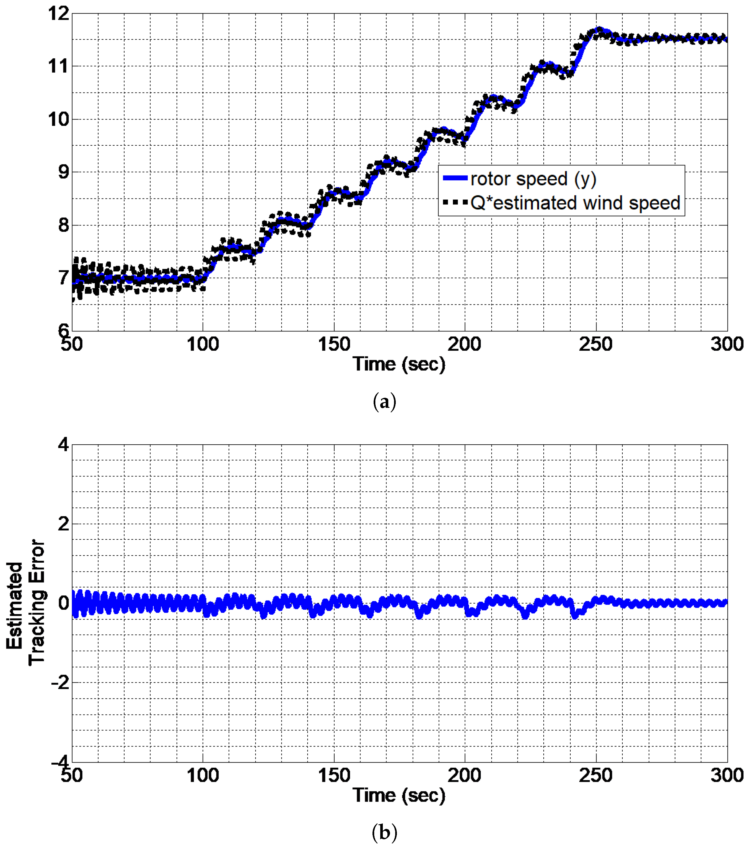
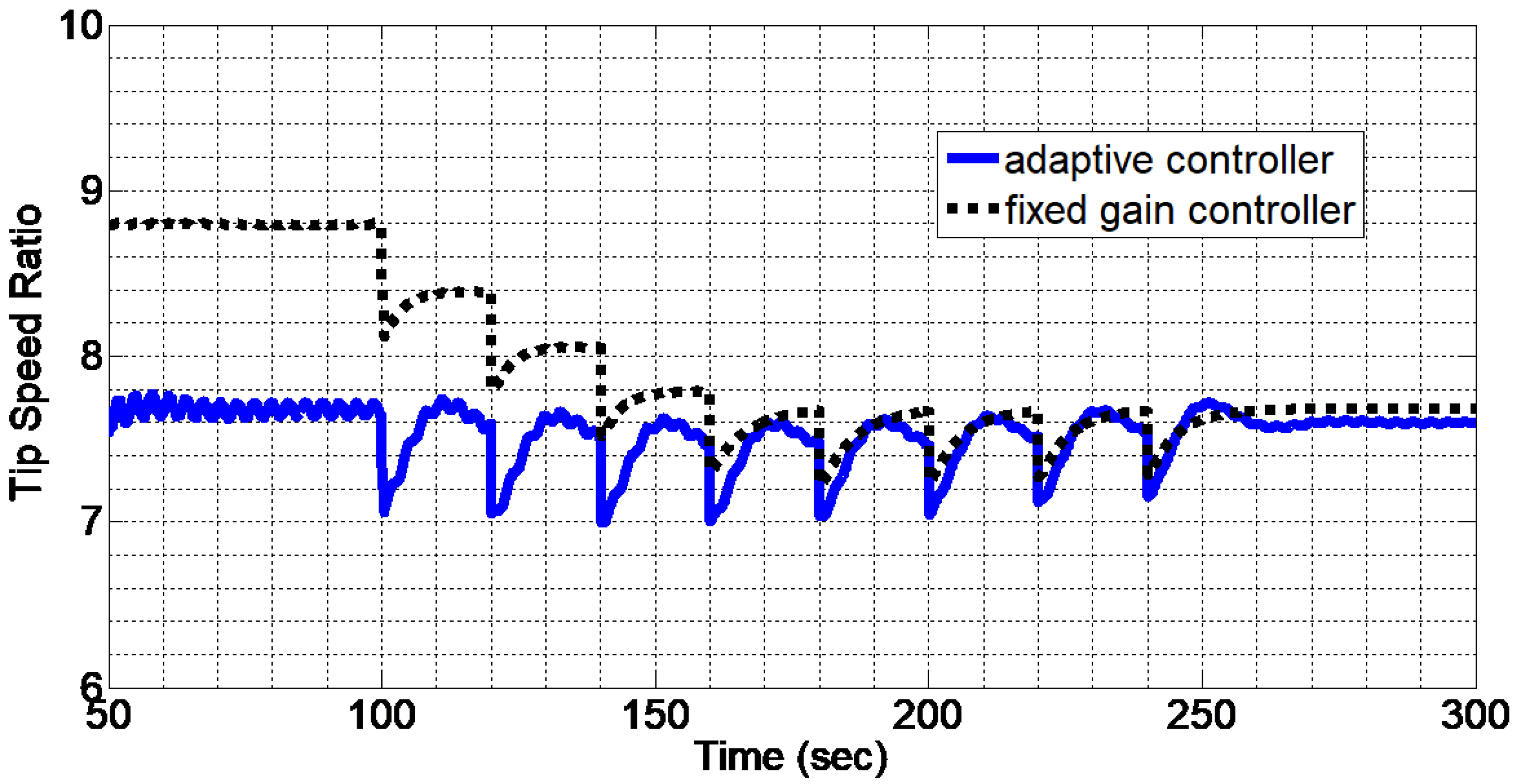
5. Illustration of Adaptive State Feedback

The proposed adaptive state feedback was used for tip-speed-ratio tracking of the NREL’s 5 MW wind turbine model [31]. This is a horizontal-axis wind turbine with a rotor radius of 63 m. It has a rated wind speed of 11.4 m/s, a rated rotor speed of 12.1 rpm, and a rated tip-speed ratio of 7.55 (this is the tip-speed ratio for maximum power extraction). It is a nonlinear wind turbine model; however, the full-order model for this wind turbine consists of 31 states when linearized at a certain operating point, and all of these are stable in Region II operation. As described previously, our aims are to augment the disturbance generator to the lower-order plant model, to estimate the corresponding states along with the wind speed, and to use this lower-order model as an adaptive state feedback for the full-order nonlinear model. The estimated wind speed, on the other hand, is used for adaptive tip-speed-ratio tracking. The schematic of the proposed estimator/controller is shown in Figure 1. The input for the wind turbine is the generator torque ($T_g$), and the rotor speed ($\mathsf{\Omega }$) is assumed as the measured variable.

The desired lower-order model containing three states arising from the generator Deegres of Freedom (DoF) and drivetrain DoF was generated by linearizing the nonlinear model at a blade pitch angle of $0^{\circ }$ and wind speed of 8 m/s. A step wind-speed profile ranging from 6 to 11 m/s was used to investigate the performance of the proposed controller. Ideally, any positive values of gains ${\gamma }_e$, ${\gamma }_D$, and ${\gamma }_z$ would be sufficient for stability of the feedback system. However, these values affect the system transients as well as the overall performance. For this particular case, we used a trial and error method to obtain satisfactory values of these gains, as we have not yet developed a systematic way to tune the gains. The performance of the proposed adaptive controller is compared to that of existing baseline PID torque controllers [31]. As stated previously, one of the main aims of this simulation was to estimate the wind speed from the rotor speed measurement using the disturbance generator model of Equation (7) and the state estimation Equation (10).

A step wind profile was used as the input to the system, and the corresponding wind estimation is presented in Figure 2. This figure shows that the proposed disturbance generator model and estimation scheme are capable of estimating the wind speed closely.

The next objective was to track the tip-speed ratio (an optimum value of 7.45 for this particular wind turbine) of the wind turbine to maximize the power capture.

Figure 3 indicates that the proposed adaptive controller is very effective in tracking the desired tip-speed ratio regardless of the large fluctuation in the wind speed.

Driving the estimated tracking error (Equation (12)) to zero is another objective of the proposed adaptive controller. Figure 4 shows that the rotor speed is very close to the quantity $Q{u}_D$ and that the resulting estimated tracking error (${\widehat{e}}_y=\mathsf{\Omega }-Q{u}_D$) is close to zero.

6. Conclusions

We have extended a class of adaptive disturbance tracking controllers developed by Balas et al. to incorporate state and wind-speed estimation and adaptive state feedback. This adaptive controller requires an ASPR system to retain stability and convergence. Therefore, we proved that the augmentation of the state and disturbance does not alter the ASPR properties of the system, thereby preserving its stability. The stability analysis was performed under the assumption that the system is LTI, although the implementation of the controller is not restricted to LTI systems so long as the nonlinear system retains ASPR properties when linearized within the set of operating points, as demonstrated by Li et al. [29]. The simulation results obtained using the NREL’s nonlinear wind turbine model show that the proposed control system is more effective compared to the baseline PID controller.

As presented by Li [29] and Yuan [30], one way to analyze the ASPR property of a nonlinear system is to linearize it at different operating points and verify whether the system is non-minimum-phase and whether the product of matrices $CB$ is positive. However, this results in an infinite number of operating points to be analyzed. One of the future endeavors is to incorporate nonlinear systems directly into analysis. Additionally, the theory does not reveal the optimal values of gains in gain adaption equations. A systematic study on finding effective values of gains to satisfy certain control performance is another research direction that we would like to explore.

References

1. Laks, J.H.; Pao, L.Y.; Wright, A.D. Control of wind turbines: Past, present, and future. In Proceedings of the American Control Conference, St. Louis, MO, USA, 10–12 June 2009; pp. 2096–2103. [Google Scholar]
2. Bossanyi, E. Wind turbine control for load reduction. Wind Energy 2003, 6, 229–244. [Google Scholar] [CrossRef]
3. Johnson, K.E.; Pao, L.Y.; Balas, M.J.; Fingersh, L.J. Control of variable-speed wind turbines: Standard and adaptive techniques for maximizing energy capture. IEEE Control Syst. 2006, 26, 70–81. [Google Scholar] [CrossRef]
4. Jonkman, J.; Butterfield, S.; Musial, W.; Scott, G. Definition of a 5-MW Reference Wind Turbine for Offshore System Development; Technical Report; National Renewable Energy Laboratory (NREL): Golden, CO, USA, 2009.
5. Wright, A.D. Modern Control Design for Flexible Wind Turbines; Technical Report; National Renewable Energy Laboratory (NREL): Golden, CO, USA, 2004.
6. Gao, R.; Gao, Z. Pitch control for wind turbine systems using optimization, estimation and compensation. Renew. Energy 2016, 91, 501–515. [Google Scholar] [CrossRef]
7. Sloth, C.; Esbensen, T.; Stoustrup, J. Robust and fault-tolerant linear parameter-varying control of wind turbines. Mechatronics 2011, 21, 645–659. [Google Scholar] [CrossRef]
8. Fragoso, S.; Garrido, J.; Vázquez, F.; Morilla, F. Comparative analysis of decoupling control methodologies and H∞ multivariable robust control for variable-speed, variable-pitch wind turbines: Application to a lab-scale wind turbine. Sustainability 2017, 9, 713. [Google Scholar] [CrossRef]
9. Schlipf, D.; Schlipf, D.J.; Kühn, M. Nonlinear model predictive control of wind turbines using LIDAR. Wind Energy 2013, 16, 1107–1129. [Google Scholar] [CrossRef]
10. Song, D.; Yang, J.; Dong, M.; Joo, Y.H. Model predictive control with finite control set for variable-speed wind turbines. Energy 2017, 126, 564–572. [Google Scholar] [CrossRef]
11. Jaramillo-Lopez, F.; Kenne, G.; Lamnabhi-Lagarrigue, F. A novel online training neural network-based algorithm for wind speed estimation and adaptive control of PMSG wind turbine system for maximum power extraction. Renew. Energy 2016, 86, 38–48. [Google Scholar] [CrossRef]
12. Narayana, M.; Sunderland, K.M.; Putrus, G.; Conlon, M.F. Adaptive linear prediction for optimal control of wind turbines. Renew. Energy 2017, 113, 895–906. [Google Scholar] [CrossRef]
13. Hatami, A.; Moetakef-Imani, B. Innovative adaptive pitch control for small wind turbine fatigue load reduction. Mechatronics 2016, 40, 137–145. [Google Scholar] [CrossRef]
14. Wen, J.T.Y.; Balas, M.J. Robust adaptive control in Hilbert space. J. Math. Anal. Appl. 1989, 143, 1–26. [Google Scholar] [CrossRef]
15. Fuentes, R.J.; Balas, M.J. Direct adaptive rejection of persistent disturbances. J. Math. Anal. Appl. 2000, 251, 28–39. [Google Scholar] [CrossRef]
16. Fuentes, R.J.; Balas, M.J. Robust model reference adaptive control with disturbance rejection. In Proceedings of the 2002 American Control Conference, Anchorage, AK, USA, 8–10 May 2002; Volume 5, pp. 4003–4008. [Google Scholar]
17. Balas, M.; Fuentes, R.; Erwin, R. Adaptive control of persistent disturbances for aerospace structures. In Proceedings of the AIAA Guidance, Navigation, and Control Conference and Exhibit, Dever, CO, USA, 14–17 August 2000; p. 3952. [Google Scholar]
18. Matras, A.L.; Flowers, G.T.; Fuentes, R.; Balas, M.; Fausz, J. Suppression of persistent rotor vibrations using adaptive techniques. J. Vib. Acoust. 2006, 128, 682–689. [Google Scholar] [CrossRef]
19. Frost, S.A.; Balas, M.J.; Wright, A.D. Direct adaptive control of a utility-scale wind turbine for speed regulation. Int. J. Robust Nonlinear Control 2009, 19, 59–71. [Google Scholar] [CrossRef]
20. Balas, M.; Li, Q.; Peterman, R. Adaptive disturbance tracking control for large horizontal axis wind turbines in variable speed region II operation. In Proceedings of the 48th AIAA Aerospace Sciences Meeting Including the New Horizons Forum and Aerospace Exposition, Orlando, FL, USA, 4–7 January 2010; p. 248. [Google Scholar]
21. Balas, M.; Thapa, K.; Li, Q. Adaptive disturbance tracking control for large horizontal axis wind turbines with disturbance estimator in Region II operation. In Proceedings of the ASME Wind Symposium, Orlando, FL, USA, 4–7 January 2011. [Google Scholar]
22. Magar, K.S.T.; Balas, M.J.; Frost, S.A. Adaptive Disturbance Tracking Control With Wind Speed Reduced Order State Estimation for Region II Control of Large Wind Turbines. In Proceedings of the ASME 2012 Conference on Smart Materials, Adaptive Structures and Intelligent Systems, Stone Mountain, GA, USA, 19–21 September 2012; pp. 329–333. [Google Scholar]
23. Magar, K.T.; Balas, M.J.; Frost, S.A. Direct adaptive torque control for maximizing the power captured by wind turbine in partial loading condition. Wind Energy 2016, 19, 911–922. [Google Scholar] [CrossRef]
24. Balas, M.; Fuentes, R. A non-orthogonal projection approach to characterization of almost positive real systems with an application to adaptive control. In Proceedings of the American Control Conference, Boston, MA, USA, 30 June–2 July 2004; Volume 2, pp. 1911–1916. [Google Scholar]
25. Wilson, R.E.; Lissaman, P. Applied Aerodynamics of Wind Power Machines; Oregon State University: Corvallis, OR, USA, 1974. [Google Scholar]
26. Wang, N.; Johnson, K.E.; Wright, A.D. FX-RLS-based feedforward control for LIDAR-enabled wind turbine load mitigation. IEEE Trans. Control Syst. Technol. 2012, 20, 1212–1222. [Google Scholar] [CrossRef]
27. Johnson, C. Theory of disturbance-accommodating controllers. Control Dyn. Syst. 1976, 12, 387–489. [Google Scholar]
28. Thapa Magar, K.; Balas, M.; Feng, Y.; Frost, S. Adaptive Pitch Control for Speed Regulation of Floating Offshore Wind Turbine: Preliminary Study. In Proceedings of the 51st AIAA Aerospace Sciences Meeting including the New Horizons Forum and Aerospace Exposition, Grapevine, TX, USA, 7–10 January 2013; p. 454. [Google Scholar]
29. Li, N. Adaptive Control of Flow Over Wind Turbine Blade. Ph.D. Thesis, University of Wyoming, Laramie, WY, USA, 2013. [Google Scholar]
30. Yuan, Y.; Tang, J. Adaptive pitch control of wind turbine for load mitigation under structural uncertainties. Renew. Energy 2017, 105, 483–494. [Google Scholar] [CrossRef]
31. Jonkman, J.M.; Buhl, M.L., Jr. Development and verification of a fully coupled simulator for offshore wind turbines. In Proceedings of the 45th AIAA Aerospace Sciences Meeting and Exhibit, Reno, NV, USA, 8–11 January 2007. [Google Scholar]
Figure 1. Schematic of the estimator/controller implementation.
Energies 10 02145 g001
Figure 2. True and estimated wind speed.
Energies 10 02145 g002
Figure 3. Tip-speed-ratio comparison between existing Proportional-Integral-Derivative (PID) controller and proposed adaptive controller.
Energies 10 02145 g003
Figure 4. (a) Rotor speed; (b) estimated tracking error.
Energies 10 02145 g004