Abstract
The growing development of hybrid electric vehicles (HEVs) has seen the spread of architectures with transmission based on planetary gear train, realized thanks to two electric machines. This architecture, by continuously regulating the transmission ratio, allows the internal combustion engine (ICE) to work in optimal conditions. On the one hand, the average ICE efficiency is increased thanks to better loading situations, while, on the other hand, electrical losses are introduced due to the power circulation between the two electrical machines mentioned above. The aim of this study is then to accurately evaluate electrical losses and the average ICE efficiency in various operating conditions and over different road missions. The models used in this study are presented for both the Continuously Variable Transmission (CVT) architecture and the Discontinuously Variable Transmission (DVT) architecture. In addition, efficiency maps of the main components are shown. Finally, the simulation results are presented to point out strengths and weaknesses of the CVT architecture.
1. Introduction
The increasing spread of medium size HEVs in the market has been led by CVT architectures equipped with a power-split device (PSD) able to continuously vary the transmission ratio thanks to the synergy with two motor-generators. This architecture is sketched in Figure 1, the main components are: internal combustion engine (ICE), two motor-generators (MG1 and MG2), planetary gear train, i.e., Sun gear (S), Ring gear (R), Carrier gear (C), and the battery (B).
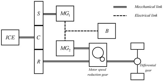
Figure 1.
CVT architecture.
In HEVs, the alternative to this structure is given by a discontinuously variable transmission (DVT) equal to that used in conventional vehicles, typically with six different values of transmission ratio. This architecture is sketched in Figure 2 (note that only one motor-generator is used).
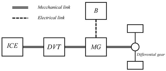
Figure 2.
DVT architecture.
The optimal energy management of the two transmission is fundamental to provide drive comfort and reduce fuel consumption. In scientific literature, one can find various studies on the implementation of optimal control logics, regarding the two architectures described.
In [1], an optimized control logic for the power split device (PSD) based architecture is proposed. In [2], a particular energy management system (EMS) is studied for the DVT architecture. Both the CVT structure and the DVT structure are considered for the optimization logic described in [3]. Many variables affect the optimization of the entire hybrid powertrain; in particular, the driving style can play a crucial role, as analyzed in [4]. In [5,6], more sophisticated methods based on neural networks and fuzzy logic are proposed.
Thus, it is then important to study optimal control techniques, but to evaluate the energy virtuosity of CVT based vehicles, analyzing electrical losses is essential. In [7,8,9], experimental tests were conducted with the aim of determining the efficiency of electric drives used in the HEVs available on the market today. Knowing this parameter is a key step in designing control logic aiming at optimizing these components [10]. Indeed, the CVT architecture allows an optimal energy management of the ICE, but at the cost of certain of electrical losses which are absent in the DVT architecture. Thus, one can find various works on the PSD based vehicles in scientific literature, however, they do not deal with a combined evaluation of electrical losses and ICE efficiency improvement deriving from the CVT system.
The main aim of this paper is to quantify these losses in every possible operating condition and compare them with the ICE energy savings obtainable by continuously regulating the transmission ratio. Firstly, the PSD model is presented; secondly, the electrical losses model is shown; and, finally, the EMS is described. In addition, a brief description is reported of the MATLAB/Simulink (2017b, Mathworks, Natick, MA, USA) DVT and CVT powertrain models.
Particular attention is paid during the results analysis not only to the electrical-loss quantification but also to the ICE management in both architectures.
In fact, to compare the energy efficiency of the two architectures a combined evaluation of electrical losses and ICE efficiency is of primary importance.
2. Model
2.1. Power Split Device Energy Model
To mathematically describe the PSD, the energy convention depicted in Figure 3 has been chosen.
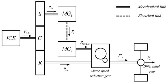
Figure 3.
CVT energy convention.
In Figure 3, the power flows are positive in the direction shown by the arrows. The analysis carried out in this study, due to the limited influence of the inertial terms of the planetary gear train components on the overall efficiency, does not consider these terms. Thus, the equations shown below are only algebraic equations and are to be considered as a stationary model.
The variable meanings are explained in Table 1.

Table 1.
Variable meanings.
It is first necessary to identify the relationship between the different velocity of the components of the PSD; Willis formula can be applied (valid if the planetary rings are merged into a single one externally toothed together):
where:
While zS and zR represent the sun gear and ring-gear-tooth number, zR is conventionally a negative number because the teeth are internal. By conveniently combining:
One obtains:
From which:
Based on the three following equations, once the value of k has been chosen, it is possible to acquire a relationship between the mechanical ring gear power and the mechanical sun gear power:
Hence:
where:
By analyzing the vehicle energy scheme, it can be immediately understood that the possible configurations in terms of power flows are various; to describe them all, this work would be overburdened. The energy configurations considered in this paper are the ones practically exploited during the vehicle usage. In addition, regenerative braking and pure electric traction are not considered here because the resulting configurations do not have any degree of freedom allowing optimization study.
Note that the input to the systems are:
Case 1 (MG1 motor, MG2 generator):
Combining the following equations:
One has:
After some passages:
Finally:
Furthermore:
Hence:
Case 2 (MG1 generator, MG2 motor):
Combining the following equations:
Repeating the same calculations as above, one has:
Case 3 (MG1 generator—only from a mechanical point of view, MG2 generator):
This particular configuration is rather frequent and it occurs in low sun gear velocity situations; in this case, the mechanical power delivered by the sun gear is not enough to overcome electrical losses in MG1, hence MG2 has to provide the remaining power. Thus:
Since the torque of the two motor generators is determined in each configuration, and their speed is known thanks to the Willis formula, once the ratio k is found (goal of the optimization process, see Section 2.3), the electrical losses can be computed (as shown in Section 2.2), and all the other variables of interest can easily be obtained.
2.2. Electrical Losses and Internal Combustion Engine Modeling
The aim of this paper being to evaluate losses in the CVT system to implement a control logic able to consider these losses, similar to that proposed in [10], the modeling of electric machines and their converters is of primary importance.
As regards electrical machines, electrical losses were modeled exploiting the results presented in [11]. These loss data are available for a specific size permanent magnet synchronous motor, in order to use these results for machines of different size (torque, speed), and losses were put in per unit, as suggested in [12]. The losses in the inverters were estimated starting from the results shown in [13], which were interpolated in accordance to that proposed in [14] and finally put in per unit.
By doing so, these maps can be used in the simulation environment for machines of different (but comparable) size.
Hence, a look up table was created for each contour map; these look up tables are formed by almost 10,000 points. To obtain a halfway loss value, linear interpolation is used. This was implemented thanks to available interpolation blocks in Matlab/Simulink environment.
The electrical losses of each electric drive are presented in per unit in Figure 4.
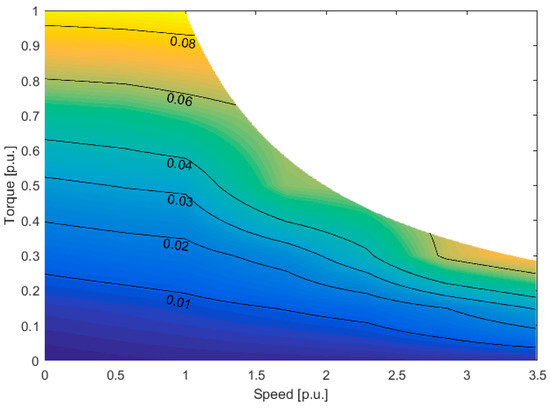
Figure 4.
Electric drive losses in per unit (p.u).
Please note that the speed value 1 is not for the maximum speed but for the base speed instead.
To evaluate the ICE efficiency, the spark ignition engine presented in [15] was considered; the fuel consumption data available in [15] were elaborated to obtain the efficiency map. This contour map is shown in Figure 5.
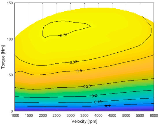
Figure 5.
ICE efficiency contour map.
2.3. CVT Powertrain Efficiency Optimization
The goal of this study is to obtain for each couple (wheel speed and wheel torque) the optimal transmission ratio k able to minimize fuel consumption. This process is not a mere search for the k value which maximizes the ICE efficiency, but it is a broader study aiming at the maximization of the entire powertrain. In fact, given the same power delivered to the wheels, the electrical losses must be compensated by a higher ICE power generation with its consequent consumption increase. To carry out this optimization process, a MATLAB/Simulink model in accordance to that proposed at Section 2.1 and Section 2.2 was created. A sufficiently numerous finite set of couples (wheel speed and wheel torque) was created to consider the variable k a continuous kopt = kopt(ωw; Tw). The PSD model and the ICE model were necessary to perform the optimization. Therefore, a combination of different value of ωw and Tw were provided as input to the model, together with all the possible k values to evaluate the fuel consumption in every operating condition. The k value, corresponding to the minimum value of fuel consumption for that particular operating condition, was then selected as a kopt value. The logical scheme of this process is represented in Figure 6.
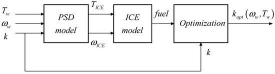
Figure 6.
CVT optimization conceptual scheme.
Thanks to the code implemented, the optimal transmission ratio function of wheel speed and wheel torque was found. In particular, due to the model implemented, this function is a “collection” of steady state points. The optimization result is shown in Figure 7.
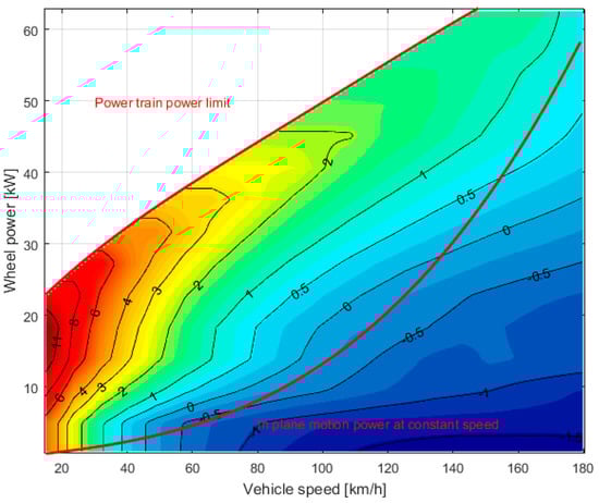
Figure 7.
k steady state function for each operating condition—CVT.
The ICE work points deriving from the optimization process are shown in Figure 8a. In Figure 8b, the ICE work points declared by Toyota are shown [16]. It is easy to notice how the optimization result is the same as that declared by Toyota, and it basically corresponds to the ICE efficiency maximization; in other terms, the electrical losses do not count in the optimization process (although they are not negligible), if compared to the losses in the ICE power generation. Please note that this conclusion could not have been drawn a priori.
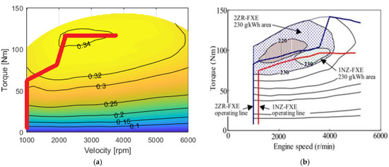
Figure 8.
(a) ICE optimal work points; and (b) Toyota ICE work points (Reprint with permission [16]; Copyright 2012, VDI-Verlag).
2.4. DVT Powertrain Effciency Optimazation
The DVT powertrain optimization is a simpler process compared to the previous one; indeed, there is only one variable to optimize, i.e., the ICE efficiency (equivalent to the fuel consumption). It is sufficient to find for each couple (wheel speed and wheel torque) the transmission ratio able to satisfy the ICE range of functioning and to maximize its efficiency. The result of this optimization process is shown in Figure 9.
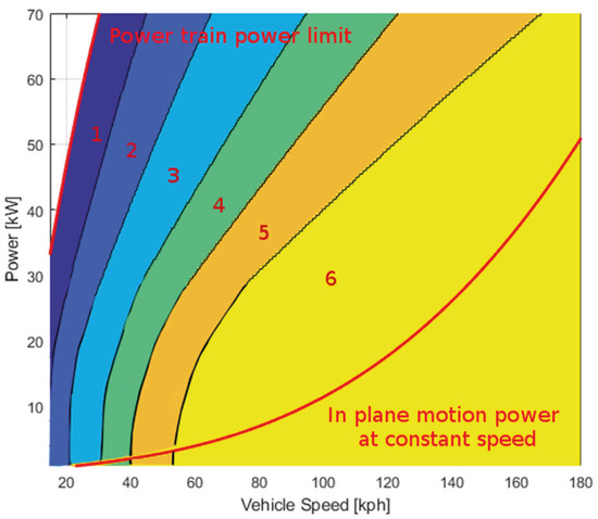
Figure 9.
Optimal transmission ratio—DVT.
2.5. MATLAB/Simulink Model
2.5.1. Power Split-Device Vehicle MATLAB Simulink Model
To quantify the variable of interest, the implementation of the two powertrain models in MATLAB/Simulink was necessary. In Figure 10, the CVT powertrain model is shown while the DVT powertrain model is shown in Figure 11. The battery and its control system were neglected because they do not intervene in the computation of the electrical losses due to the realization of the transmission ratio k. Indeed, the role played by this component is the same in the two architectures; the same control logics can be applied and the benefits deriving from regenerative braking and electric traction are identical in both configurations.
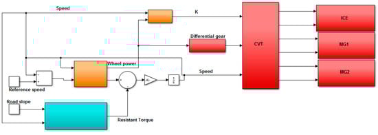
Figure 10.
CVT MATLAB/Simulink model.
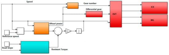
Figure 11.
DVT MATLAB/Simulink model.
Implementing control logic for the storage system management and its accurate modeling are important, for instance, to determine fuel consumption, emission evaluation, etc. It is not necessary in this study but would be to evaluate the electrical losses associated with the realization of the transmission ratio (in the CVT architecture) and to determine the average ICE efficiency.
The red blocks in Figure 10 represent the model of physical components, the light blue block computes the resistant torque and the orange blocks implement the control logic. The complete model is necessary to simulate the powertrain response to the various road missions with respect to the reference speed and road slope. On the contrary, the light blue block is not necessary to calculate electrical losses and the ICE efficiency; therefore, the inputs in this case are the vehicle speed and the wheel power directly, which are provided as ramp signals to compute the desired parameters in each operating condition.
2.5.2. DVT MATLAB/Simulink Model
Similar to that implemented for the CVT architecture, one model for the DVT powertrain was created. The same considerations previously mentioned, as far as the role of each block is concerned, remain valid.
2.6. Vehicle Features
The vehicle features are reported in Table 2; the parameters common to the two architectures are characterized by the same values to allow a fair comparison.
Table 2.
Vehicle features.
2.7. Road Mission Features
As previously described, the electrical-loss evaluation is firstly carried out considering every possible operating condition of the powertrain. However, some operating conditions are much more important and more frequent than others during the real usage of the vehicle, hence the importance of the simulation of the powertrain response over actual road missions.
The vehicle speed and road slope data (inputs to the vehicle models) were experimentally collected via GPS, in particular these missions were distinguished in: urban mission, extra urban mission and a highway mission. In addition, simulations were also carried out on three American type approval tests (HWFET, US06, and UDD6).
The main characteristics of these three missions are listed in Table 3.
Table 3.
Vehicle features.
Detailed results are only reported for real missions; however, the powertrain efficiency is evaluated on the totality of the described missions.
3. Results
3.1. Electrical Losses in Power-Split Device
3.1.1. Electrical Losses in Power-Split Device over Different Operating Condition
Once the optimization is performed, it is possible to obtain the electrical losses in operating conditions necessary to realize the desired transmission ratio k. Note that only the operation of the two electric drives during the transmission ratio realization is analyzed. The operation of the two machines during regenerative braking and electric traction is not relevant to this study, as it is that of the battery as mentioned above.
Therefore, the electrical losses considered in this study are only associated with the CVT architecture because of the electrical power circulation between the two motor-generators necessary to realize the transmission ratio, thus these losses are completely absent in the DVT powertrain.
In Figure 12a, the electrical losses are plotted again for each operating condition; it is also useful to compare these losses with the power generated by the ICE. In Figure 12b, the same losses are shown in percentage with respect to the power delivered by the ICE in the same work point. One can easily notice how relevant these losses are; in addition, most of the powertrain operating conditions are placed in areas characterized by losses higher than 10%.
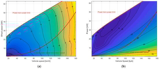
Figure 12.
(a) Electrical losses (kW) as a function of wheel power and vehicle speed; and (b) electrical losses (%) in percentage with respect to ICE power, as a function of wheel power and vehicle speed.
3.1.2. Electrical Losses in Power-Split Device over Different Real-Road Missions
With the aim of quantifying the impact of these losses during real operating conditions, it is useful to locate the work points of the different missions. The urban mission work points are shown in Figure 13 on a zoomed area of the electrical-loss contour map. Figure 14 shows the extra urban mission work points, while Figure 15 shows the ones associated with the highway mission.
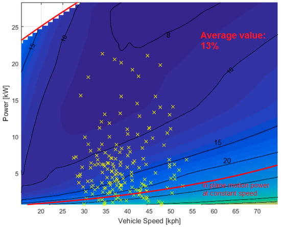
Figure 13.
Urban mission work points on the electrical-loss (%) contour map.
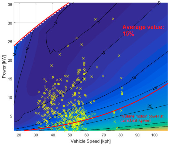
Figure 14.
Extra-urban mission work points on the electrical-loss (%) contour map.
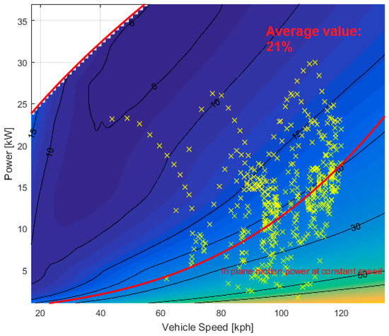
Figure 15.
Highway mission work points on the electrical-loss (%) contour map.
As simulations pointed out, electrical losses have a considerable effect on the powertrain efficiency. The results obtained for the missions considered show that electrical losses are nearly 13% of the total energy delivered by the ICE and reach 21% for highway missions.
3.2. ICE Efficiency
3.2.1. ICE Efficiency over Different Operating Condition
It is shown in Section 3.1 that the amount of electrical losses in the CVT architecture can reach 20% of the ICE generated power. However, this structure allows the engine to work more efficiently by continuously varying the transmission ratio. Thus, to perform a comprehensive energy evaluation of both powertrain typologies, an in-depth study of the ICE efficiency during real operating conditions in both cases is crucial.
In Figure 16, the global ICE efficiency is shown as a function of vehicle speed and wheel power. This contour map does not plot the ICE efficiency as a function of its speed and torque but rather plots the efficiency as a function of road variables; this result can only be obtained once the transmission ratio is known for every operating condition. Hence, the relationship between ICE variables (torque and speed) and road variables (vehicle speed and wheel power) is unique.
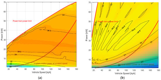
Figure 16.
ICE efficiency [%] contour map as a function of road variables: (a) CVT; and (b) DVT.
In other terms, these plots were obtained starting from the same ICE efficiency contour map (Figure 5) applying the control logics presented in Section 2.3 and Section 2.4.
In Figure 16b, one can notice six areas characterized by efficiency values higher than 34.5%. These areas correspond to the six transmission ratios available for the DVT architecture. It can also be immediately seen in Figure 16a that the efficiency area of values higher than to 34.5% is much wider and it extends even for high vehicle speed. In particular, Figure 16a, as previously described, is another way of looking at Figure 8a. In fact, only the work points on that red line are those entirely plotted here with respect to road variables.
3.2.2. ICE Efficiency over Different Real Road Mission
Similar to Section 3.1.2, the ICE efficiency was evaluated over real road missions; this analysis is indeed extremely important because it allows us to draw conclusions on CVT structure energy virtuosity. Specifically, it shows whether the ICE efficiency increase can compensate for the electrical losses.
In Figure 17, Figure 18 and Figure 19, the vehicle work points are placed on a zoomed area of the two ICE efficiency contour maps. What was previously mentioned is thus confirmed: the CVT architecture in fact enables the ICE to work at higher efficiency values. In particular, this benefit is more relevant during high-speed missions thanks to the overdrive.
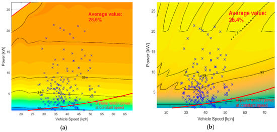
Figure 17.
Urban mission work points: (a) CVT; and (b) DVT.
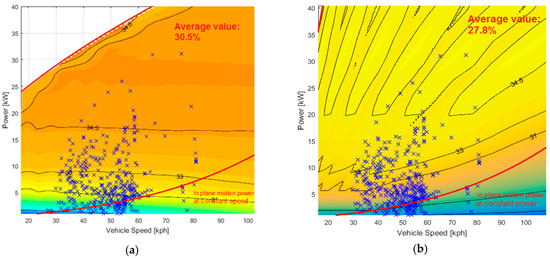
Figure 18.
Extra-urban mission work points: (a) CVT; and (b) DVT.
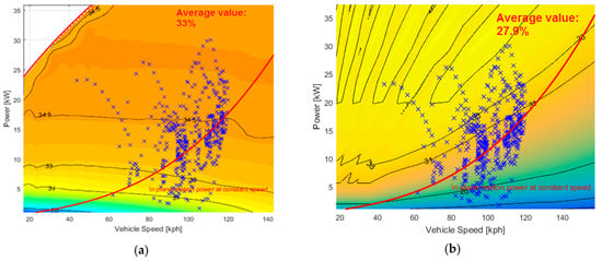
Figure 19.
Highway mission work points: (a) CVT; and (b) DVT.
3.3. Powertrain Global Efficiency
To quantify the combined effect of electrical losses due to the transmission ratio realization and the ICE efficiency increase, the powertrain global efficiency, defined by the following equation, is computed over all the missions presented:
This value accounts for the ICE efficiency, the electrical losses and the mechanical efficiency of the transmission and differential gear. The powertrain efficiency values of the different missions are listed in Table 4.
Table 4.
Powertrain efficiency over different road missions.
4. Conclusions
The PSD energy model and losses in the electric drives are modeled in this paper. Subsequently, the MATLAB/Simulink model for the CVT and DVT architectures are described. The CVT electrical-loss contour map is then presented. To estimate the impact of the two different transmissions on the ICE operating conditions, contour maps of the ICE as a function of road variables are obtained for both the parallel configurations by knowing the transmission ratio associated for each work point (acquired by the fuel consumption minimization process).
Finally, three real road missions were simulated to locate the work points on the different contour maps, evaluating strengths and weaknesses of both architectures.
The results obtained confirmed what was previously speculated: the CVT configuration allows the engine to work at higher efficiency rate, but at the cost of consistently high electrical losses.
Again, the CVT architecture is characterized by an 8% ICE efficiency increase in the urban mission (28.6% vs. 26.4%), 9% efficiency increase in the extra-urban mission and 16% in the highway mission.
Nevertheless, this improvement is not sufficient to compensate for the large amount of electrical losses generated by the continuously variable transmission on the three missions: 13%, 15% and 21% of the ICE generated energy.
Although the CVT based hybrid electric vehicles are widely spread in the medium size car market sector, they do not prove to be the best energy solution.
Further developments of this study will include the experimental validation of the results achieved via simulations by means of prototyping in collaboration automotive companies.
Acknowledgments
The authors would like to wholeheartedly thank Alessandro Pini Prato for his suggestions, assistance, and encouragement throughout this work.
Author Contributions
Damiano Lanzarotto and Massimiliano Passalacqua created the models. Renato Procopio and Mario Marchesoni provided useful information about the permanent magnet synchronous motors and revised the manuscript while Matteo Repetto provided useful data on the ICE. Massimiliano Passalacqua, Damiano Lanzarotto and Andrea Bonfiglio implemented the models in the simulator, performed the simulations and elaborated the results. Damiano Lanzarotto and Massimiliano Passalacqua wrote the paper.
Conflicts of Interest
The authors declare no conflict of interest.
References
- Xia, C.; Du, Z.; Zhang, C. A single-degree-of-freedom energy optimization strategy for power-split hybrid electric vehicles. Energies 2017, 10, 896. [Google Scholar] [CrossRef]
- Lee, H.; Park, Y.I.; Cha, S.W. Power management strategy of hybrid electric vehicle using power split ratio line control strategy based on dynamic programming. In Proceedings of the 2015 15th International Conference on Control, Automation and Systems (ICCAS), Busan, Korea, 13–16 October 2015; pp. 1739–1742. [Google Scholar]
- Fan, J.; Zhang, J.; Shen, T. Map-based power-split strategy design with predictive performance optimization for parallel hybrid electric vehicles. Energies 2015, 8, 9946–9968. [Google Scholar] [CrossRef]
- Lee, S.; Choi, J.; Jeong, K.; Kim, H. A study of fuel economy improvement in a plug-in hybrid electric vehicle using engine on/off and battery charging power control based on driver characteristics. Energies 2015, 8, 10106–10126. [Google Scholar] [CrossRef]
- Chen, Z.; Mi, C.C.; Xu, J.; Gong, X.; You, C. Energy management for a power-split plug-in hybrid electric vehicle based on dynamic programming and neural networks. IEEE Trans. Veh. Technol. 2014, 63, 1567–1580. [Google Scholar] [CrossRef]
- Abdelsalam, A.A.; Cui, S. A fuzzy logic global power management strategy for hybrid electric vehicles based on a permanent magnet electric variable transmission. Energies 2012, 5, 1175–1198. [Google Scholar] [CrossRef]
- Burress, T.A.; Coomer, C.L.; Campbell, S.L.; Seiber, L.E.; Marlino, L.D.; Staunton, R.H.; Cunningham, J.P. Evaluation of the 2007 Toyota Camry Hybrid Synergy Drive System; ORNL/TM2007/190, Revised; UT-Battelle, Oak Ridge National Laboratory: Oak Ridge, TN, USA, 2008.
- Burress, T.A.; Coomer, C.L.; Campbell, S.L.; Wereszczak, A.A.; Cunningham, J.P.; Marlino, L.D. Evaluation of the 2008 Lexus LS 600h Hybrid Synergy Drive System; ORNL/TM-2008/185; UT-Battelle, Oak Ridge National Laboratory: Oak Ridge, TN, USA, 2009.
- Burress, T.A.; Campbell, S.L.; Coomer, C.L.; Ayers, C.W.; Wereszczak, A.A.; Cunningham, J.P.; Marlino, L.D.; Seiber, L.E.; Lin, H.T. Evaluation of the 2010 Toyota Prius Hybrid Synergy Drive System; Technical Report ORNL/TM2010/253; Oak Ridge National Laboratory (ORNL), Power Electronics and Electric Machinery Research Facility: Oak Ridge, TN, USA, 2011.
- Son, H.; Park, K.; Hwang, S.; Kim, H. Design methodology of a power split type plug-in hybrid electric vehicle considering drivetrain losses. Energies 2017, 10, 437. [Google Scholar] [CrossRef]
- Pellegrino, G.; Vagati, A.; Guglielmi, P.; Boazzo, B. Performance comparison between surface-mounted and interior pm motor drives for electric vehicle application. IEEE Trans. Ind. Electron. 2012, 59, 803–811. [Google Scholar] [CrossRef]
- Mahmoudi, A.; Soong, W.L.; Pellegrino, G.; Armando, E. Efficiency maps of electrical machines. In Proceedings of the 2015 IEEE Energy Conversion Congress and Exposition (ECCE), Montreal, QC, Canada, 20–24 September 2015; pp. 2791–2799. [Google Scholar]
- Kim, H.; Chen, H.; Zhu, J.; Maksimović, D.; Erickson, R. Impact of 1.2kv SiC-MOSFET EV traction inverter on urban driving. In Proceedings of the 2016 IEEE 4th Workshop on Wide Bandgap Power Devices and Applications (WiPDA), Fayetteville, AR, USA, 7–9 November 2016; pp. 78–83. [Google Scholar]
- Passalacqua, M.; Lanzarotto, D.; Repetto, M.; Marchesoni, M. Advantages of using supercapacitors and silicon carbide on hybrid vehicle series architecture. Energies 2017, 10, 920. [Google Scholar] [CrossRef]
- Königstein, A.; Grebe, U.D.; Wu, K.-J.; Larsson, P.-I. Differentiated analysis of downsizing concepts. MTZ Worldw. 2008, 69, 4–11. [Google Scholar] [CrossRef]
- Adachi, S.; Hagihara, H. The Renewed 4-Cylinder Engine Series for Toyota Hybrid System. In Proceedings of the 33rd International Vienna Motor Symposium, Vienna, Austria, 26–27 April 2012; pp. 1–24. [Google Scholar]
© 2017 by the authors. Licensee MDPI, Basel, Switzerland. This article is an open access article distributed under the terms and conditions of the Creative Commons Attribution (CC BY) license (http://creativecommons.org/licenses/by/4.0/).