Article

Distribution and Presence of Polymers in Porous Media

1
School of Energy Resources, China University of Geosciences (Beijing), No. 29 Xueyuan Road, Haidian District, Beijing 100083, China
2
Key Laboratory of Marine Reservoir Evolution and Hydrocarbon Enrichment Mechanism, Ministry of Education, Beijing 100083, China
3
Beijing Key Laboratory of Unconventional Natural Gas Geological Evaluation and Development Engineering, Beijing 100083, China
*
Author to whom correspondence should be addressed.
Energies 2017, 10(12), 2118; https://doi.org/10.3390/en10122118
Submission received: 6 September 2017 / Revised: 1 December 2017 / Accepted: 6 December 2017 / Published: 13 December 2017

Abstract

:
In order to better utilize the residual polymers formed after polymer flooding, the distribution and the presence of the polymers after polymer flooding were studied. This paper studied the vertical and plane distribution of the hydrophobically-associating polymer in addition to measuring the parameters after polymer flooding, which is important for numerical reservoir simulation. The results showed that the polymers mainly enter into the high permeability zone and distribute in the mainstream line area with only a small portion in the wing area. Based on the comparison of various experimental methods, double-slug experiments were chosen to measure the inaccessible pore volume and retention, which is considered to be the most accurate, most time-consuming and most complex method. Following this, we improved the processing method of experimental data by reducing it to one experiment with two parameters. At the same time, we further enhanced the accuracy of the experimental results. The results show that at 1750 mg/L, the inaccessible pore volume of the polymer is 25.8%. When the detention is 68.2 µg/g, the inaccessible pore volume constituted 22% of the total polymer, with the other 77.7% being the dissolved polymer. Moreover, the static adsorption and dynamic detention were measured, with the results showing that the static adsorption is larger than dynamic detention. Therefore, in the numerical reservoir simulation, using the static adsorption capacity instead of the dynamic detention is unreasonable. The double-slug method was chosen since it is more accurate for the determination of various parameters. Meanwhile, in order to enhance the accuracy of results, we improved the treatment of data.

1. Introduction

During the development of an oilfield, oil recovery can be improved obviously by injecting polymers [1,2,3,4,5] into the formation, and some scholars have provided extensive reviews of the polymer concentrations, viscosities, and bank sizes used during existing and previous polymer floods. It is believed that the polymer flooding technology needs to be improved in many aspects, such as the risk of mechanical degradation, the produced fluid processing, the large number of polymers remaining in the formation after polymer flooding [6,7], and so on. The residual polymer will be industrial waste if it is not fully utilized. Furthermore, a large gap will occur between predicted results and the actual situation without experimental evidence since the dynamic prediction needs to be adjusted according to the experience of the reservoir engineer [8]. The distribution of the polymer in the formation is affected by many factors, such as heterogeneity [9], polymer concentration [10], polymer molecular weight [11], injection rate [12] and so on. Clarifying the distribution of polymers can provide the criteria for the next step to fully utilize the residual polymer. The presence [13,14,15,16] of polymers in porous media can be divided into two parts: polymers in the inaccessible pore volume (VIP) or polymers in the accessible pore volume. The latter has two states: detention [17] (including adsorption and captation) and dissolved polymers, which is shown in Figure 1. The inaccessible pore volume occurs primarily because polymer molecules are large relative to solvent molecules and pores in the reservoir rock [18]. The VIP for polymer flooding has both positive and negative effects [19,20]. It is known that VIP affects the rate of movement of polymer molecules through the medium. It is also probable that solvent interactions affect the flow and dispersion of solvent in which the polymers are dissolved. Table 1 shows a model [21], which depicts the serious impact of VIP on the polymer flooding development index and on deciding follow-up operations. However, due to the complexity of the experiment, the VIP is hardly measured with the requirement for adjustment of parameters in the numerical models. If the VIP is not chosen to be a suitable value, it will lead to an inaccurate prediction of the polymer breakthrough time [22].
In polymer flooding, polymer retention is defined to include the combined effects of polymer adsorption on rock and mechanical entrapment of the polymer in pores. Polymer retention can have a major impact on polymer-slug propagation and economics. Manichand and Seright [23] calculated that a 1240-ppm polymer solution exhibiting a retention value of 100 mg/g would require injection of 50% more polymer to reach a target distance in a formation (relative to the case for no polymer retention). They also reported field polymer (HPAM) retention values ranging from 50 to 250 mg/g for the Tambaredjo polymer flood in Suriname. Detention is also an important basis for the engineering design and the input data for the numerical reservoir simulation [24,25], which affects the formation permeability reduction factor. The numerical simulation often uses static adsorption instead of the dynamic detention, although there is a significant difference between them. The static adsorption is unable to represent the real reservoir retention law, because it does not measure the losses caused by the mechanical trapping and hydrodynamic retention of polymers in the pore. Sometimes we use the material balance method [13] to measure the dynamic retention, but the error of material balance method is relatively large. The material balance method consists of injecting polymer into the core until the adsorption is saturated, and the amount of polymer injected minus the amount of polymer produced is the amount of dynamic retention. Because of the polymer remaining in the injection pipeline, the experimental error is particularly large. It is frequently difficult to obtain the VIP and dynamic retention for polymer flooding numerical simulations, which seriously affects the results of numerical simulation and prediction of the dynamic field.
The distribution of polymers was studied in a macroscopic view, while the parameters, such as VIP and detention, are determined in microscopic scales. The primary objectives were (1) to study the distribution of polymer concentration and viscosity in the formation, (2) to determine the microscopic state of existence which provides basic parameters for a mathematical model, (3) to prove that the double-slug method is feasible, and that one experiment can yield two data sets including VIP and dynamic retention of the polymer at the same time. This study has significance in guiding the numerical simulation of polymer and dynamic monitoring.

2. Materials and Method

2.1. Experimental Materials

The chemicals include hydrophobic associating polymers (molecular weight of 1250 × 104 g/mol, solid content of about 90% and degree of hydrolysis of about 25%), the simulated oil, of which the oil viscosity is 73 mPa·s at 65 °C, and the API of crude oil is 15. For the experimental water, we prepared the synthetic brine according to the current polymer flooding situation of the oilfield, with the composition shown in Table 2, and other materials shown in Table 3.
The experimental instruments mainly include two kinds of artificial core: one is a cylindrical core and the other is a three-dimensional slab model, and the model’s parameters are shown in Table 3. In laboratory experiments, we frequently use artificial cores, including the slab model, instead of the precious natural cores. The artificial cores consist of quartz sand and cement. The method for measuring the permeability of the slab model is as follows: in the process of core manufacture, we make a very big model first, and then cut a small piece, which can be made into one dimensional core for example a cylindrical core. We can measure the permeability of the small core. The composition of the whole slab model is the same, so the permeability of the small core represents the permeability of the whole slab model.

2.2. Methods

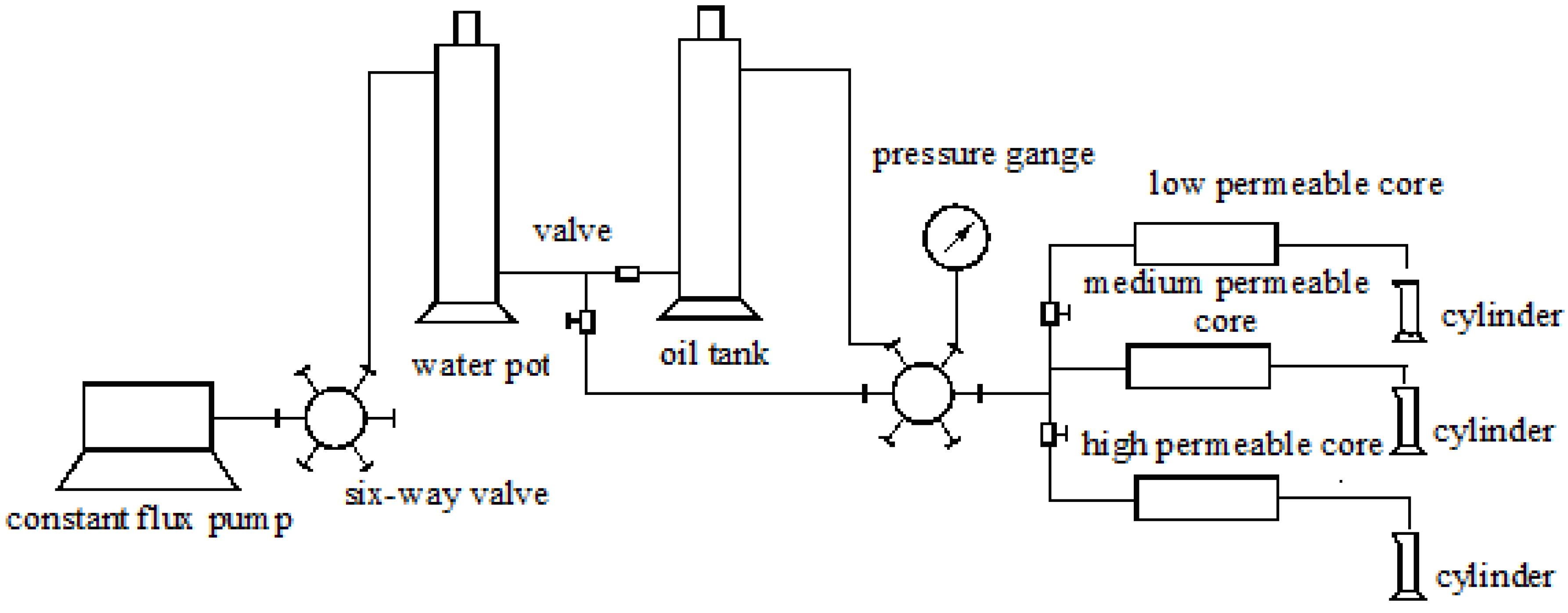
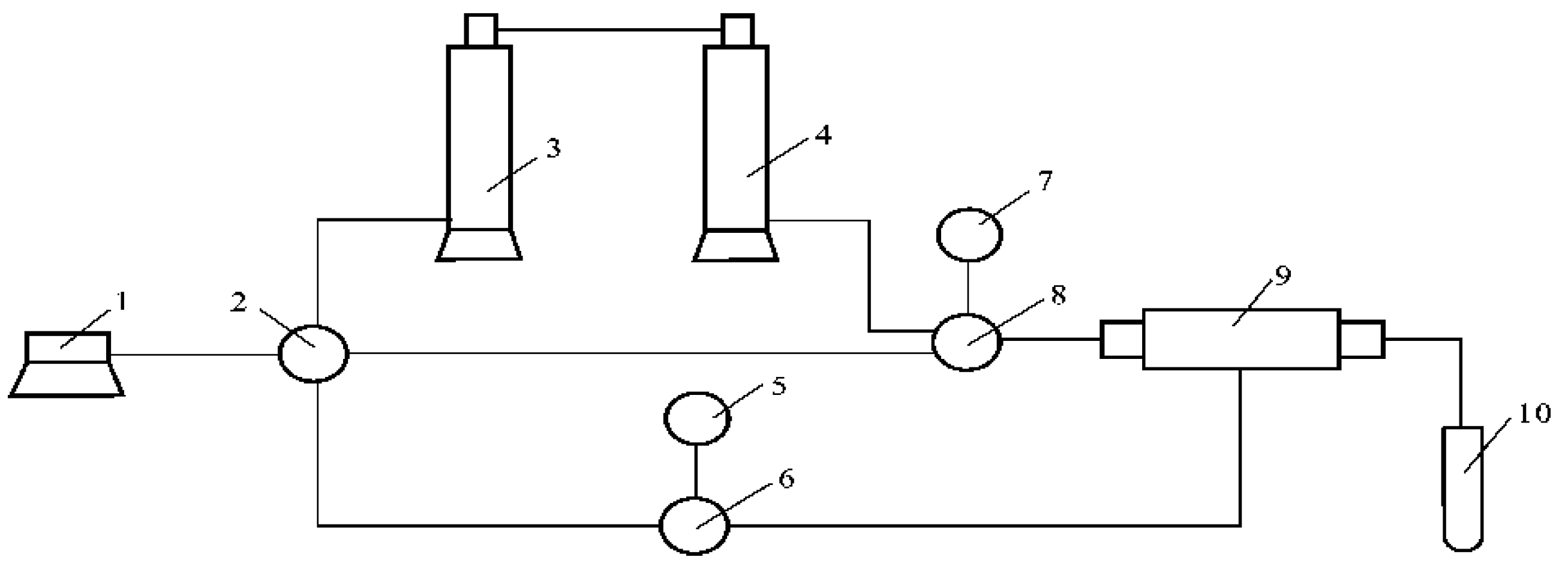
2.2.1. Three Parallel Core Experiments

The temperature is set at 65 °C, which is under the reservoir conditions, while the injection rate is 0.5 mL/min. Parallel cores were used to determine the effect of heterogeneity on the polymer distribution, with the schematic drawing of the flow shown in Figure 2. The testing procedure includes the following steps. ① Fill the pack with sand and obtain the dry weight, before saturating it with water, measuring the wet weight and calculating the pore volume. ② Flood with water and measure the permeability after the pressure is stable, with the permeability of cores being 300 × 10−3 μm2, 900 × 10−3 μm2 and 2700 × 10−3 μm2 respectively. ③ Inject the oil into the core to establish irreducible water saturation (short for Swi). ④ Install the three cores in parallel and flood with water until the water cut is 98%. ⑤ Inject the polymer solution at 1500 mg/L to a maximum of 0.57 PV. According to the oilfield development plan, the injection process will be ended after injection of the 0.57 PV polymer. ⑥ Record the fluid output volume of each core, which is equal to the injection volume of the polymer.

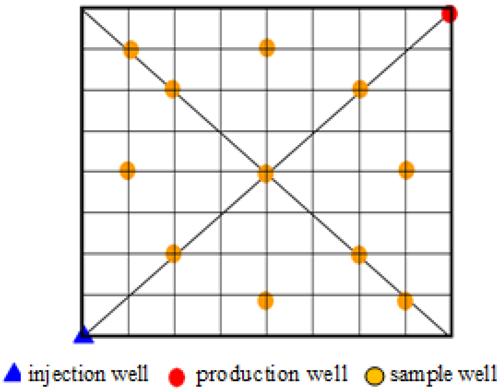
2.2.2. Three-Dimensional Slab Model Experiment

The three-dimensional slab model was used to measure the polymer’s viscosity and concentration distribution after polymer flooding, with the model parameters shown in Table 4. The model and well spacing pattern is shown in Figure 3. The test procedure involves the following steps. ① Measure the dry weight of the model. ② Saturate model with water, measure the wet weight of the model and calculate the pore volume of the model. The value of pore volume equals the ratio of the difference between wet weight and dry weight to water density. ③ Calculate the initial oil saturation (short for Soi) after injecting the simulated oil in the model, which equals the ratio of volume of injected oil to pore volume of the model. ④ Inject polymer solution at 1500 mg/L to a maximum of 0.57 PV. ⑤ Take the samples from the sampling wells, before measuring the viscosity and concentration. ⑥ Draw the isograms of viscosity and concentration using Sufer8.0 software (Golden Software, Golden, CO, USA).

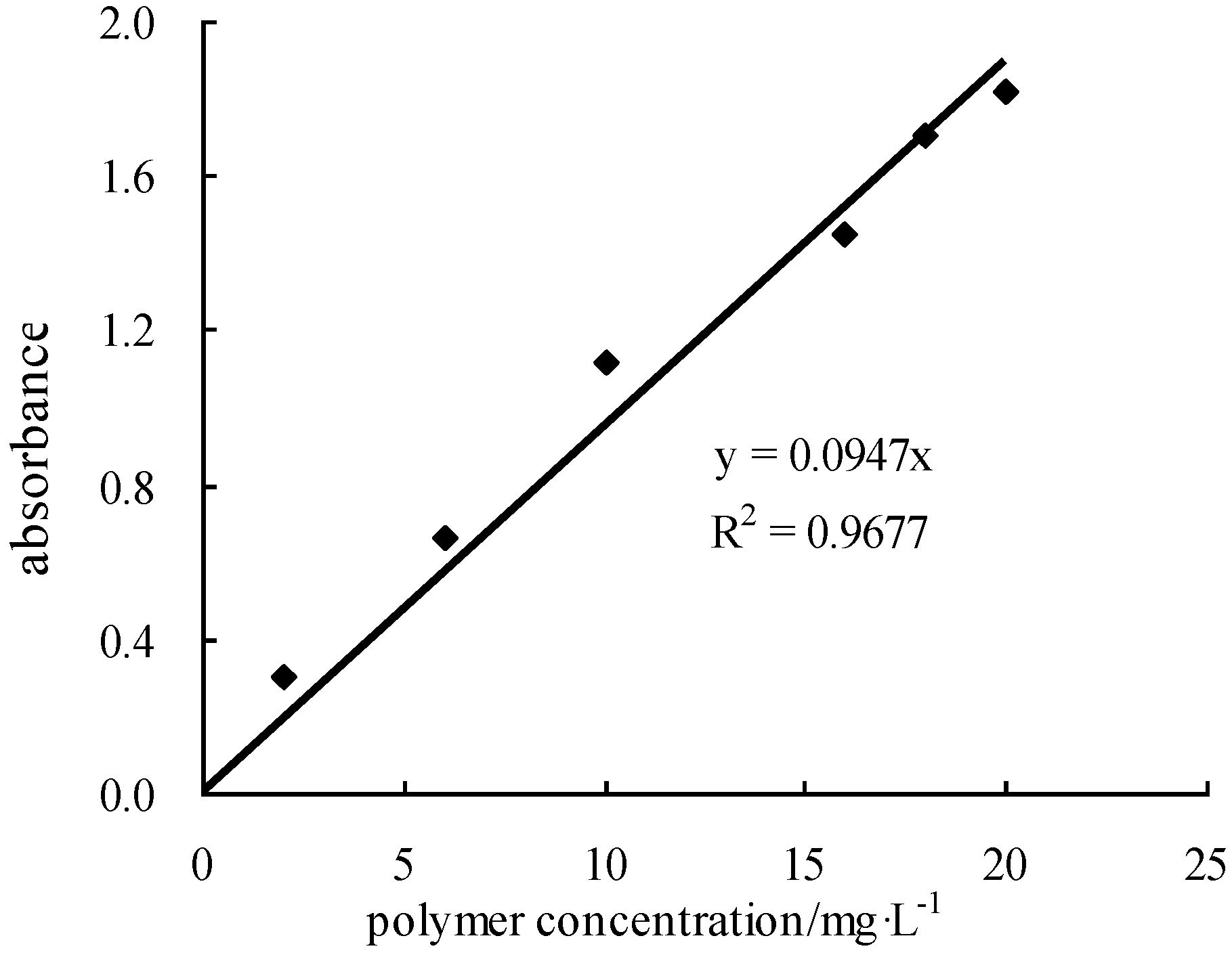
2.2.3. Polymer Concentration Determination Method

The starch–cadmium iodide method [26] is used to measure the polymer concentration, with the concentration–absorbance standard curve shown in Figure 4. The method can directly determine the polymer concentration, with simple operation and a fast detection rate. R2 is the linear correlation coefficient, which represents the linear correlation of two columns of data.

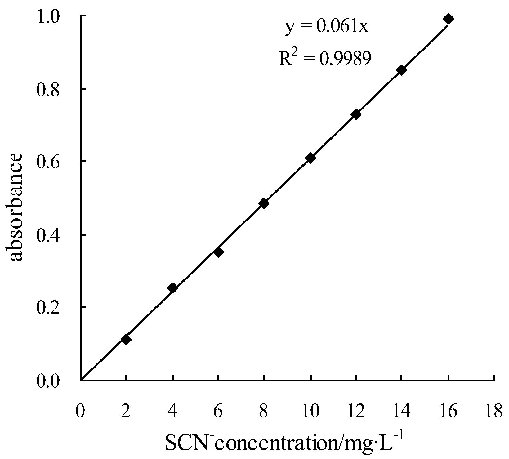
2.2.4. Potassium Thiocyanate Tracer Determination Method

The spectrophotometer method [27] was applied to determine the concentration of the potassium thiocyanate tracer, with the tracer concentration–absorbance standard curve shown in Figure 5.

2.2.5. Static-Equilibrium Adsorption

The static-adsorption tests were performed on sand particles at 65 °C, and the particle size of quartz sand was 0.25–1 mm. The polymer solutions were added to clean, dry sands with a liquid: solid ratio of approximately 5:1. Then, the mixtures were stirred for 15 min to ensure adequate contact, and left quiescent for 24 h. Next, the supernatant was decanted from the mixtures and centrifuged at 300 r/min for further separation. Then, the fully separated polymer solutions were tested by the starch–cadmium iodine method [26]. The static-adsorption was determined by the polymer concentration change of the solution, volume of polymer solution, and the mass of sand particles:
The   static   adsorption = the   polymer   concentration   change   × volume   of   polymer   solution the   mass   of   sand   particles

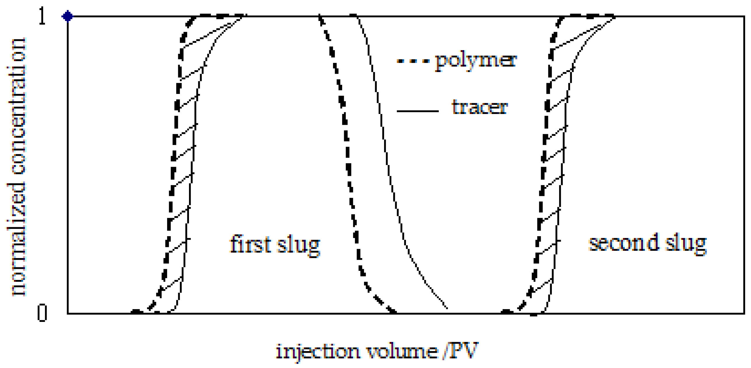
2.2.6. Double-Slug Experiments

The experiments described in this paper were all single-phase displacements of polymer solutions through consolidated sandstone. All the cores were prepared by evacuating and saturating with brine, with the pore volumes of the cores measured at this time. The experimental floods reported were conducted in severe steps, as depicted in Figure 6. The test procedure included the following steps. ① Prepare 500 mg/L polymer solution and select potassium thiocyanate (short for KSCN) as the tracer at a concentration of 300 mg/L. ② Blend the 1750 mg/L polymer solution and 300 mg/L KSCN solution, before injecting the first mixed fluid slug into the core. ③ Monitor the pressure changes and sample the outflow mixed fluid, before determining the concentration of polymer and thiocyanate root (short for SCN). ④ Continuously inject the mixed fluid system until the pressure is stable, before injecting the formation water until there is no polymer in the effluent. ⑤ Inject the second mixed fluid slug into the core, which contains 500 mg/L polymer solution and 300 mg/L KSCN solution. ⑥ Monitor the pressure changes and sample the outflow of mixed fluid, before determining the concentration of polymer and SCN. ⑦ Continuously inject the mixed fluid system until the pressure is stable, before injecting the formation water until there is no polymer in the effluent. The schematic diagram of the experimental results is shown in Figure 7. Although the tracer dissolves in the polymer solution, the curve is still separated. Two reasons lead to the first slug separation, one is the inaccessible pore volume caused the forefront of the polymer slug advance to break through, the other is the detention caused the forefront of the polymer slug to be delayed. Separation of the second slug was caused by the inaccessible pore volume. In Section 3.2.1, we will explain the reason why in detail and explain how to get the parameters for VIP and polymer retention.

3. Results and Discussion

3.1. Distribution of Polymer

3.1.1. Vertical Distribution

Using the three parallel cores which permeability (short for K) are shown in Table 5, the variation coefficient of permeability is 0.78 and the total pore volume is 44.3 mL. After injecting 0.57 pore volume (short for PV) polymer solution into the three parallel cores, the polymer concentration is 1750 mg/L. Table 5 shows that 68.3% of the polymer solution flows into the high permeability layer. Because the polymer solution is not a Newtonian fluid, the results presented in this table do not follow Darcy’s Law.

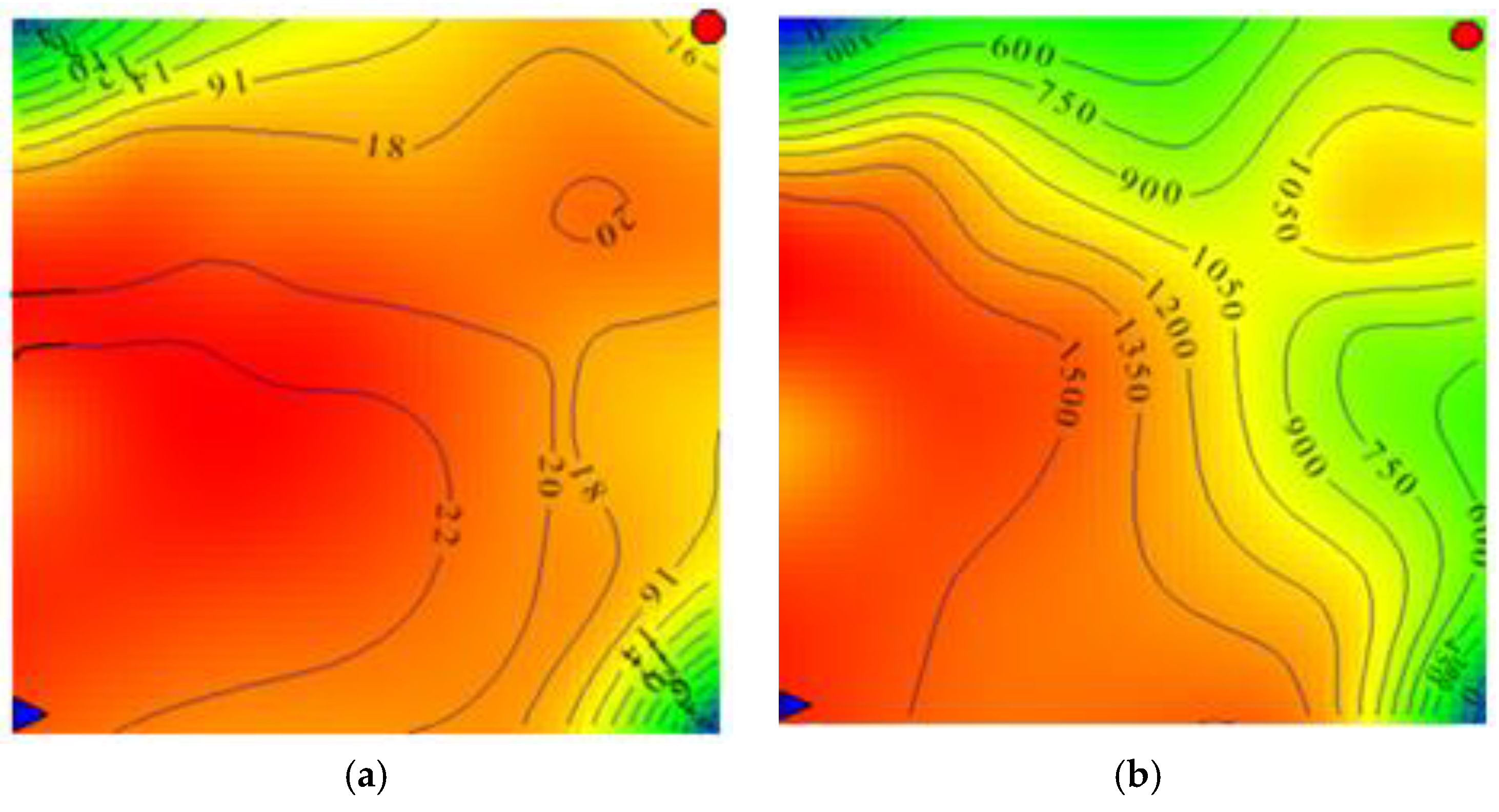
3.1.2. Plane Distribution

The three-dimensional slab model experiment is applied to determine the viscosity and concentration distribution after the polymer flooding. The relationship between viscosity of the polymer solution and concentration is shown in Figure 8. The viscosity distribution is shown in Figure 9a with units of mPa·s, while the concentration distribution is shown in Figure 9b with units of mg/L. The Energies 10 02118 i001 represents the injection well and Energies 10 02118 i002 represents the production well.
Figure 9 shows that the polymer mainly distributes in the injection–production well mainstream line area. One reason is that the polymer flooding front is constantly diluted by the formation water. The other is that regarding the retention of the polymer, the farther from the injection well, the lower the concentration. Therefore, we deduced that the residual oil mainly distributes in the two wings away from the mainstream line of injection and production wells.

3.2. Present State of Polymers

This paper mainly determines the parameters to characterize the polymers’ present state, including inaccessible pore volume, detention (including adsorption and capture) and dissolved polymers.

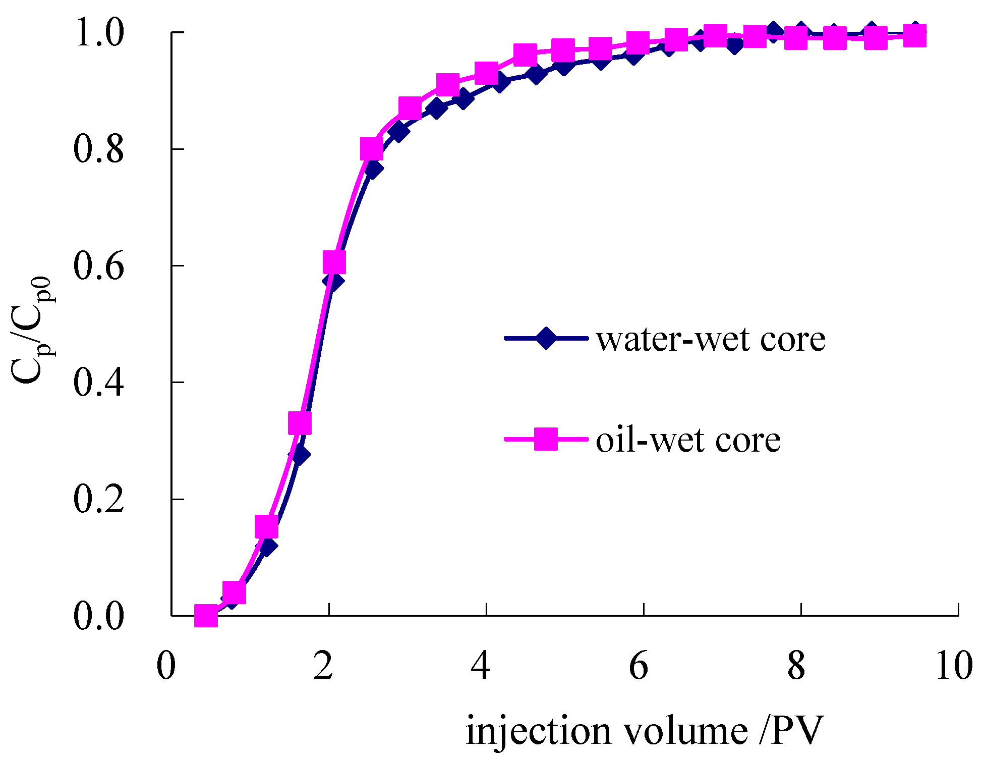
3.2.1. Determination of Inaccessible Pore Volume

The VIP and dynamic retention can be obtained by a double-slug experiment. We used the double-slug method to determine the VIP of polymers at 65 °C and 1750 mg/L, and the experimental process follows 2.2.6, with the core parameters shown in Table 6. The gas slippage effect causes the significant difference between brine and gas permeabilities. Often, the gas permeability is larger than the brine permeability in the same rock.
The normalized concentration of polymer is defined as:
Cp* = Cp/Cp0
where Cp is the concentration of the produced polymer and Cp0 is the initial concentration of the injected polymer.
The normalized concentration of tracer SCN is defined as:
Cs* = Cs/Cs0
where Cs is the concentration of produced SCN and Cs0 is the initial concentration of injected tracer. When the injection volume is in the interval [0 PV, 10.27 PV], the polymer concentration profile and tracer concentration profile separates. There are two reasons that lead to this separation: one is the inaccessible pore volume causing the forefront of the polymer slug to break through, while the other is the detention causing a delay in the forefront of the polymer slug. Figure 10 shows that the inaccessible pore volume has a greater impact on separation. When the injection volume is in the interval [10.27 PV, 20.13 PV], the inaccessible pore volume causes separation, but the water displacing the polymer solution leads to the inhomogeneous displacement. When the injection volume is in the interval [20.13 PV, 29.79 PV], since the polymer has been balanced in the first polymer slug, the inaccessible pore volume causes the separation, while the polymer solution displacing the water leads to a uniform displacement. C/C0 means the normalized concentration. Therefore:
VIP = 20.13 29.79 ( C p * C s * ) dPV / PV   =   25.8 %

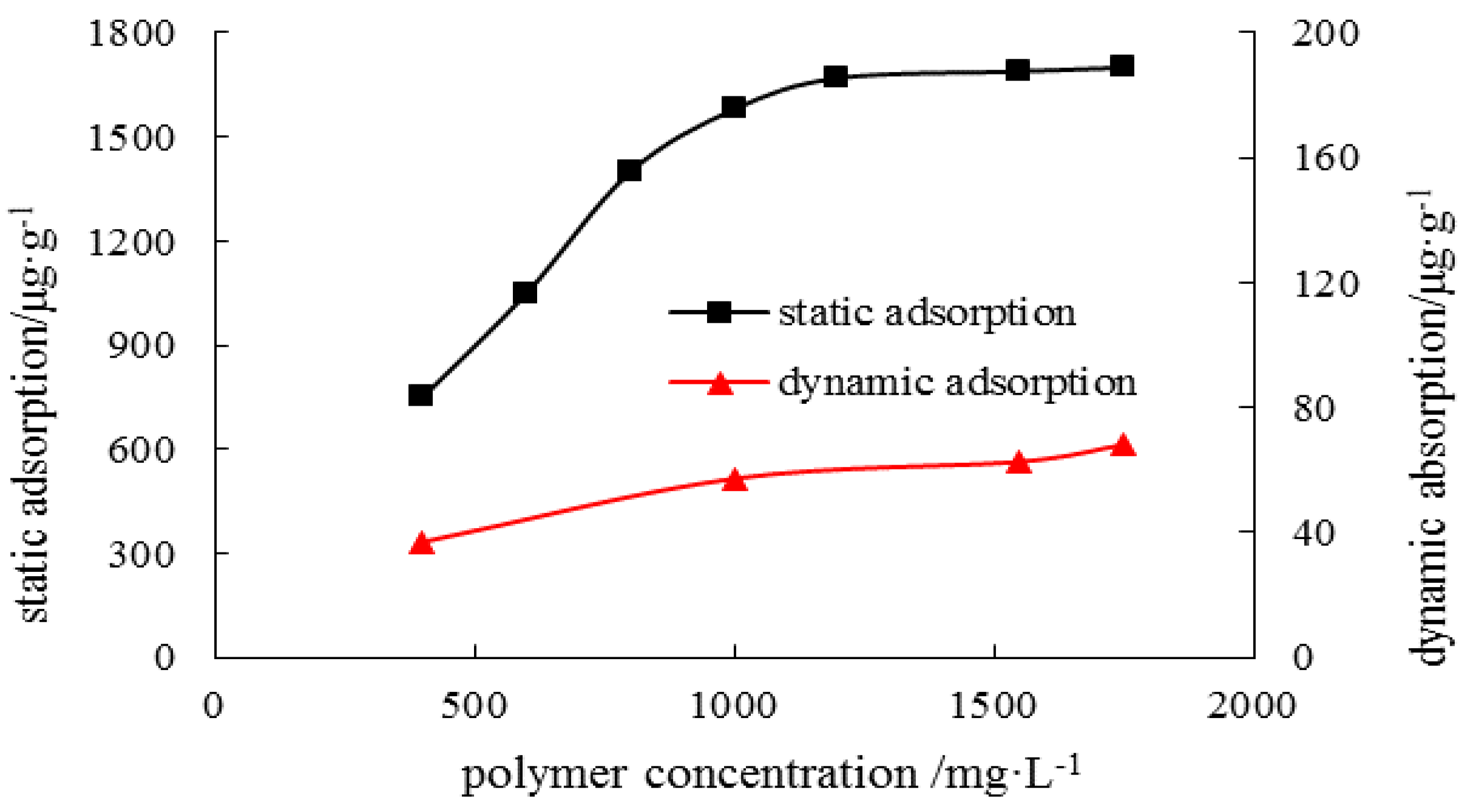
3.2.2. Dynamic Retention Characteristics

Dynamic Retention of the Polymer

(1) Measurement of Dynamic Retention
The experimental data of the first slug was used in the double-slug method (the equivalent of the large slug method [28]), which improved experimental precision and reduced the number of experiments. In order to avoid the situation of low mobility fluid being displaced by high mobility fluid in the second interval, the third interval was used instead of the second. After integration, the retention of the polymer is 68.2 μg/g when its concentration was 1750 mg/L.
(2) Contrast of Dynamic Retention and Static Adsorption
In order to simplify the operation of the reservoir numerical simulation, the converted number of static adsorption was often used instead of the dynamic adsorption. In this paper, the static adsorption of the polymer solution at different concentrations at 65 °C and the dynamic retention of the polymer were measured with the gas permeability at 2500 × 10−3 μm2. The results are shown in Figure 11. The method in a previous study [14] was used in measuring the static adsorption, when the experimental temperature was 65 °C, the solid−liquid ratio was 1:5 and the particle size of quartz sand was from 0.25 to 1 mm.
Figure 11 shows that the static adsorption and retention capacity increase significantly with an increase in polymer concentration. However, both the variation law and the magnitude are different. The static adsorption is consistent with the Langmuir adsorption law, while the dynamic retention shows a linear relationship with polymer concentration. The ratio of static adsorption and dynamic retention varies with polymer concentration, but it is about 25 in the range of concentration measured.

Dynamic Adsorption of the Polymer

Using cores with the same specifications as in Section “Dynamic Retention of the Polymer”, which were saturated with methyl silicone oil for 48 h, the wettability reversed. The oil film limited the polymer adsorption in the rock surface [29]. The polymer solution with a concentration of 1750 mg/L was used for polymer flooding and the method of measuring retention was used in the experiment. The results are shown in Figure 12. The difference between the integration of two curves was the dynamic adsorption capacity. The dynamic adsorption was 43.4 μg/g, accounting for 63.6% of retention.

Dynamic Trapping of the Polymer

The dynamic retention of the polymer includes dynamic trapping of the polymer and dynamic adsorption of the polymer. The dynamic retention is 68.2 μg/g and the dynamic adsorption is 43.4 μg/g. Therefore, the dynamic trapping is 24.8 μg/g, accounting for 36.4% of retention.

Dissolution Amount of Polymer

To calculate the amount of dissolved polymer in pores after polymer flooding, the volume of the core is 1 m3, the core porosity after polymer flooding is 29.23% and the inaccessible pore volume is 25.8%. It is known that the mass concentration of the injected polymer is 1750 mg/L, so the amount of injected polymer can be calculated as:
Sandstone density equals core mass divided by core volume = dry weight of core/(length of core × cross-sectional area of core × (1 − porosity)) = 71.48/(9.45 × 4.52 × (1 − 29.23%)) = 2.36 g/cm3
The mass of core in contact with polymer is: 1 × (1 − 29.23%) × (1 − 25.8%) × 2.36 × 106 = 1.24 × 10⁶ g.
When the amount of retention is 68.2 μg/g, the total amount of retention is: 68.2 × 1.24 × 106 = 84.6 g.
The percentage of retention from total amount of polymer:
wRetention = 84.6/379 × 100% = 22.3%
The percentage of dynamic adsorption from total amount of polymer:
wdynamic adsorption = 22.3% × 63.6% = 14.2%
The percentage of the trapped polymer from total amount of polymer:
wthe trapped polymer = 22.3% − 14.2% = 8.1%
The percentage of the dissolved polymer from total amount of polymer:
wdissolved polymer = 100% − 22.3% = 77.7%

4. Conclusions

The polymer mainly enters into the high permeability zone and distributes in the main stream line area, with only a small proportion in the wing area. Therefore, we deduced that the residual oil mainly distributes in the two wings away from the mainstream line of injection and production wells.
The double slug method is feasible and can be obtained using two parameters, VIP and detention. The polymer concentration–absorbance standard curve and the tracer concentration–absorbance standard curve are the basic work.
This paper provided a complete set of polymer distribution state parameters. The results show that at 1750 mg/L, the inaccessible pore volume of the polymer is 25.8%. When the detention is 68.2 µg/g, the inaccessible pore volume constituted 22% of the total polymer, with the other 77.7% being the dissolved polymer. The dynamic adsorption in retention is 43.4 μg/g, accounting for 14.2% of the total polymer, while the dynamic trapped polymer is 24.8 μg/g, accounting for 8.1% of the total polymer. It has great significance in guiding numerical polymer simulation and dynamic monitoring.
With an increase in polymer concentration, both the dynamic retention and static adsorption increase. The dynamic detention is smaller than static adsorption and the ratio changes with polymer concentration. If the converted amount of static adsorption is used instead of the retention, the deviation is large. In the numerical reservoir simulation, using the static adsorption capacity instead of the dynamic detention is unreasonable.

Author Contributions

Juan Zhao conceived and designed the experiments, analyzed experimental data and wrote this paper. Hongfu Fan provided some suggestions and contributed materials. Qing You and Yi Jia participated in the experiment work.

Conflicts of Interest

The authors declare no conflict of interest.

References

  1. Lee, S.; Kim, D.H.; Huh, C.; Pope, G.A. Development of a Comprehensive Rheological Property Database for EOR Polymers. In Proceedings of the SPE Annual Technical Conference and Exhibition, New Orleans, LA, USA, 4–7 October 2009. [Google Scholar]
  2. Seright, R.S. How Much Polymer Should Be Injected during a Polymer Flood? Review of Previous and Current Practices. SPE J. 2016, 1–18. [Google Scholar]
  3. Huang, B.; Zhang, W.; Xu, R.; Shi, Z.; Fu, C.; Wang, Y.; Song, K. A Study on the Matching Relationship of Polymer Molecular Weight and Reservoir Permeability in ASP Flooding for Duanxi Reservoirs in Daqing Oil Field. Energies 2017, 10, 951. [Google Scholar] [CrossRef]
  4. Alsofi, A.M.; Blunt, M.J. Polymer flooding design and optimization under economic uncertainty. J. Pet. Sci. Eng. 2014, 124, 46–59. [Google Scholar] [CrossRef]
  5. Sheng, J.J.; Leonhardt, B.; Azri, N. Optimization of polymer flooding in reservoirs under bottom-water condition to maximize economic profit. J. Can. Pet. Technol. 2015, 54, 116–126. [Google Scholar] [CrossRef]
  6. Zhao, F.; Wang, Y.; Dai, C.; Ren, S.; Jiao, C. Techniques of enhanced oil recovery after polymer flooding. J. China Univ. Pet. 2006, 30, 86–89. [Google Scholar]
  7. Fu, X.; Zeng, J.; Gao, W.; Tian, C.; Lin, J. Overview of further improvement of oil recovery technology after polymer flooding. Pet. Geol. Eng. 2010, 24, 88–90. [Google Scholar]
  8. Feng, Q.; Shi, S.; Fu, X.; Dai, C.; Tang, E. Numerical simulation of the residual polymer reutilization. Acta Pet. Sin. 2010, 31, 801–805. [Google Scholar]
  9. Zhu, Y.; Cao, X.; Song, X.; Zhang, Z.; Han, Y. Research on polymer distributing law by the three-dimensional anisotropic model. Oil Drill. Prod. Technol. 2006, 28, 39–41. [Google Scholar]
  10. Xu, J.; Wang, L.; Zhu, K. Concentration distribution and variation in a polymer-flooding reservoir. Tsinghua Univ. Sci. Tech. 2002, 42, 455–457. [Google Scholar]
  11. Lu, X.; Gao, Z.H.; Zhao, X.J.; Yan, W.H. Distribution Regularities of Remaining Oil in Heterogeneous Reserviors after polymer flooding. Acta Pet. Sin. 1996, 17, 55–58. [Google Scholar]
  12. Liu, L. The Roles of residual oil Distribution and Measurement of Further Exploitation after Polymer Flooding. Master’s Thesis, Daqing Petroleum Institute, Daqing, China, 2005. [Google Scholar]
  13. Miao, J.S.; Zhao, F.L.; Li, S.; Yu, Y.H.; Chen, M. Presence and distribution of residual polymer in formation. Spec. Oil Gas Reserv. 2005, 12, 88–90. [Google Scholar]
  14. Zhang, J.; Lu, S.; Li, J.; Zhang, P.; Xue, H.; Zhao, X.; Xie, L. Adsorption Properties of Hydrocarbons (n-Decane, Methyl Cyclohexane and Toluene) on Clay Minerals: An Experimental Study. Energies 2017, 10, 1577. [Google Scholar] [CrossRef]
  15. Wan, H.; Seright, R.S. Is Polymer Retention Different under Anaerobic vs. Aerobic Conditions? In Proceedings of the SPE Improved Oil Recovery Conference, Tulsa, OK, USA, 11–13 April 2016. [Google Scholar]
  16. Zhang, G.; Seright, R.S. Hydrodynamic Retention and Rheology of EOR Polymers in Porous Media. In Proceedings of the SPE International Symposium on Oilfield Chemistry, The Woodlands, TX, USA, 13–15 April 2015. [Google Scholar]
  17. Fulin, Z. Oilfield Chemistry; China University of Petroleum Press: Dongying, China, 2000; pp. 105–149. [Google Scholar]
  18. Bhupendra, N.; Lawrence, G.; Willhite, P.; Green, D.W. The effect of inaccessible pore volume on the flow of polymer and solvent through porous media. In Proceedings of the SPE Annual Fall Technical Conference and Exhibition, Houston, TX, USA, 1–3 October 1978. [Google Scholar]
  19. Hu, B. Polymer Flooding Petroleum Production Engineering; Petroleum Industry Press: Beijing, China, 1997; pp. 27–28. [Google Scholar]
  20. Li, J.; Liu, Y.J.; Guo, S.L.; Li, B.-H. A method for calculating inaccessible pore volume of polymer. Pet. Geol. Oilfield Dev. Daqing 2008, 27, 114–117. [Google Scholar]
  21. Tang, E.; Zhang, X.; Yang, J. The effect of inaccessible pore volume on the flow of polymer solution in porous media. Pet. Geol. Recovery Effic. 2009, 16, 80–82. [Google Scholar]
  22. Cheng, T.; Pu, W. Polymer Evaluation Methods; Petroleum Industry Press: Beijing, China, 1997; p. 107. [Google Scholar]
  23. Manichand, R.N.; Seright, R. Field vs. Laboratory Polymer Retention Values for a Polymer Flood in the Tambaredjo Field. SPE Reserv. Eval. Eng. 2014, 17, 314–325. [Google Scholar] [CrossRef]
  24. Di, Q.; Shen, C.; Wang, Z.H.; Gu, C.; Shi, L.; Fanf, H. Experimental research on drag reduction of flow in micro channels of rocks using nano-particle adsorption method. Acta Pet. Sin. 2009, 30, 125–128. [Google Scholar]
  25. Zhang, G.; Seright, R.S. Effect of Concentration on HPAM Retention in Porous Media. In Proceedings of the SPE Annual Technical Conference and Exhibition, New Orleans, LA, USA, 30 September–2 October 2014. [Google Scholar]
  26. Shu, L.; Liu, J.; Lv, X.; Guo, Y. Measurement optimization of polymer concentration of polyacrymide by the starch-cadmium iodine method. Appl. Chem. Ind. 2010, 39, 1766–1782. [Google Scholar]
  27. Jing, G.-L.; Li, Y.-Q.; Yang, J. Spectrophotometric determination of concentration of ammonium. Thiocyanate Tracer Oilfield Prod. Water 2000, 17, 191–192. [Google Scholar]
  28. Li, H.-B. Characteristic Static Adsorption of Hydrophobically Associating Polymer AP from Aqueous Solution. Oilfield Chem. 2006, 23, 349–351. [Google Scholar]
  29. Broseta, D.; Medjahed, F.; Lecourtier, J.; Robin, M. Polymer adsorption/retention in porous media: Effects of core wettability on residual oil. SPE Adv. Technol. Ser. 1995, 3, 103–112. [Google Scholar] [CrossRef]
Figure 1. The present state of the polymer in strata.
Energies 10 02118 g001
Figure 2. Three parallel core experiments.
Energies 10 02118 g002
Figure 3. The well spacing pattern.
Energies 10 02118 g003
Figure 4. The polymer concentration–absorbance standard curve.
Energies 10 02118 g004
Figure 5. The tracer concentration–absorbance standard curve.
Energies 10 02118 g005
Figure 6. Double-slug experiments measuring the inaccessible pore volume. (1 = constant-flux pump; 2 = six-way valve; 3 and 4 = Intermediate container; 5 and 7 = precision pressure gauge; 6 and 8 = seat; 9 = core holder; and 10 = measuring cylinder).
Energies 10 02118 g006
Figure 7. The schematic diagram of the Double-Slug experimental results.
Energies 10 02118 g007
Figure 8. Viscosity of polymer solution against concentration.
Energies 10 02118 g008
Figure 9. Viscosity and Concentration distribution after polymer flooding. (a) viscosity distribution; (b) concentration distribution
Energies 10 02118 g009
Figure 10. The concentration profile of polymer and tracer.
Energies 10 02118 g010
Figure 11. The effect on static adsorption and dynamic adsorption of polymer concentration.
Energies 10 02118 g011
Figure 12. The dynamic adsorption of polymers.
Energies 10 02118 g012
Table 1. Effect of the inaccessible pore volume (VIP) on polymer flooding development index [21].
VIPPolymer Breakthrough Time/MonthRecovery When Water Cut at 95%/%The Additional Recovery/%
079.744.5520.35
0.1567.137.8313.63
0.2558.333.349.14
0.3550.528.854.65
0.4542.324.370.17
Notes: Table 1 comes from reference [21].
Table 2. The composition of synthetic brine.
CompositionNa+, K+Ca2+Mg2+CO32−HCO3SO42−ClTotal Salinity
content/(mg/L)3091.96276.17158.6814.21311.4885.295436.349374.12
Table 3. List of materials required for experiments.
ExperimentArtificial Core Chemicals and Materials
Three Parallel Core ExperimentsThree cylindrical cores (sectional area, 4.9 cm2; length, 9.8 cm). The water permeability of cores is 300 × 10−3 μm2, 900 × 10−3 μm2 and 2700 × 10−3 μm2polymer, constant flux pump, core holder, Brookfield DV-II rotational viscometer, pressure sensor(Haian County Petroleum Science and Technology Co., Ltd., Haian, China), precise pressure gauge, graduate, cylinder, oil tank, et al.
Three-Dimensional Slab Model ExperimentThe slab model (the model parameter is shown in Table 4.polymer, constant flux pump, core holder, Brookfield DV-II rotational viscometer (DV-II+, Brokfield, WI, USA), pressure sensor, precise pressure gauge, graduate, et al.
Polymer Concentration Determination Method polymer, sodium acetate, cadmium iodide, hydrated aluminum sulfate, saturated bromine water, soluble starch, acetic acid, sodium formate, UV-2100 spectrophotometer, BS423S millesimal balance (BS423S, Shanghai Precision Scientific Instruments Co., Ltd., Shanghai, China), et al.
Potassium Thiocyanate Tracer Determination Method tracer (potassium thiocyanate), sodium formate, nitric acid, ammonium ferrous sulfate, UV-2100 spectrophotometer (UV-2100, unico Shanghai, China), BS423S millesimal balance, et al.
Static-Equilibrium Adsorption polymer, sand, temperature controlled bath, conical flask, the chemicals and materials used in Polymer Concentration Determination Method et al.
Double-Slug ExperimentsTwo cylindrical core (sectional area, 4.9 cm2; and length,9.8 cm), and their gas permeability is 2500 × 10−3 μm2polymer, tracer (potassium thiocyanate), the chemicals and materials used in Polymer Concentration Determination Method and Potassium Thiocyanate Tracer Determination Method. constant flux pump, core holder, BS423S millesimal balance, Brookfield DV-II rotational viscometer, pressure sensor, precise pressure gauge, graduate, et al.
Table 4. The model parameters.
Gas Permeability/×10−3 μm2Size/cmPorosity/%Soii/%
250059.8 × 59.2 × 4.5830.473.1
Table 5. The results of the three parallel core experiment.
CoreK/×10−3 μm2PV/mLφ/%Polymer Injection Volume/mLInjection Volume Percentage/%
high permeable core270015.432.317.268.3
medium permeable core90014.830.86.626
low permeable core30014.129.41.55.7
Table 6. The basic parameters of core.
Length/cmCross-Sectional Area/cm2Gas Permeability/10−3 μm2Water Permeability/10−3 μm2Dry Weight/gWet Weight/gPore Volume/mLPorosity/%
9.454.522484160071.4883.9812.529.23

