1. Introduction
Swirl burners have been widely used in gas turbine combustors because of their flame stability and rapid fuel/air mixing characteristics. The intensity of swirl is decided by the swirler structure and affected by the combustion chamber shape. A high velocity annular jet is issued into the chamber along the expanded wall and a central recirculation zone is formed. Then a shear layer is created between the high velocity jet and the Center Toroidal Recirculation Zone (CTRZ) [
1,
2,
3]. The CTRZ promotes the mixing of fuel/air and serves as a flame stabilization mechanism. The swirl can trigger large scale unsteady motion known as Processing Vortex Structure (PVC) and it was reviewed to illustrate the instabilities of swirl field [
4,
5,
6,
7]. In relevant researches [
4,
5,
6,
7], motions of the vortex core along the chamber have been manifested and the motion characteristics have been described through the power spectral densities method. The results show that strong PVC is developed under isothermal conditions contributed to turbulence instability by triggering the formation of radial axial eddies.
The spray combustion of swirl burners has been widely investigated using experiments and simulation methods, in particular under lean conditions. Most of those studies focused on the atomization, combustion characteristics and emissions of combustor. Sauter Mean Diameter (SMD) of fuel droplets is generally used to evaluate the atomization quality of fuel spray. For instance, Hadef [
8,
9,
10] used Phase Doppler Anemometry (PDA) to experimentally explore the spatial distributions of fuel droplets, and then examined effects of swirler structure on droplet characteristics. Their results show that the atomization from swirl burners could become finer and dispersed rapidly in the chamber. The advantage makes ignition much easier which then improves combustion efficiency and greatly lowers pollutant emissions. Numerical simulations of swirl burners include CFD (Computational Fluid Dynamics) investigation into turbulent spray breakup, effects of droplet sizes on burning behavior and etc., with Reynolds Averaged Navier-Stokes (RANS) or Large Eddy Simulation (LES) [
11,
12,
13]. In some CFD investigations, the sub-grid scale probability density function approach has been used to account for turbulence-chemistry interactions. Zhu [
14] and Khandelwal [
15] used RANS to calculate the velocity and temperature distributions in a combustor. They reported that the Realizable
k-
ε Turbulence Model could work very well compared to Reynold’s Stress Model (RSM) for calculating turbulence. The axial velocity and radial velocity distribution at different positions showed RSM turbulence models are more sensitive to the flow field tangential variation, but with the Realizable
k-
ε Model it is much easier to solve the swirling flow. Huang [
16,
17] studied the effects of swirl flows on combustion dynamics under a lean condition. As lean combustion technology was employed in gas turbines due to environmental and efficiency concerns, they found that the high swirler number increased the turbulence intensity and the flame speed. The swirl number had no obvious influence on the frequency of acoustic oscillations, but determined the wave motion. They also found that lean combustion is a promising technology that could be used in gas turbine engines for reducing both NO
x emissions and reaction zone size, and the combustion instability phenomenon could be improved by optimizing the fuel/air mixing. With both experimental investigation and numerical simulation, Orbay [
18] and Cai [
19] examined effects of heat release on flow field characteristics. Their results suggested that the spray combustion dramatically changed the gas phase velocity distributions and decreased the recirculation zone size.
Turbulent flow fields in combustion chamber are strongly influenced by the geometry which normally has an expanding inlet and contracting outlet. Different chamber geometry might lead to different vortex breakdown processes and form different flow fields. By employing a Laser Doppler Anemometer (LDA) system for measuring the tangential and axial components of flow velocity in a circular tube with different swirl intensity [
20,
21], it was found that the influence of outlet contraction was limited under low swirl condition, such as under the swirl number
S = 0.3. Under high swirl number, effects of contraction structure had become significant. Here the swirl number is defined as [
1,
4]:
where
U is the axial velocity,
W is the tangential velocity,
Maxial is axial flux of axial momentum,
Mangular is the axial flux of the angular momentum.
High swirl burners have been widely applied in combustor due to their apparent advantages. Strong turbulence can enhance the mixing between fuel and oxidant and improve flame stability by aerodynamic anchoring of the flame, but the penalty in the increase of NO
x emissions is a difficult problem. To deal with this, swirl intensity must be regulated very carefully for implementing low emission combustion. Several attempts have been conducted by Escudier [
21] to investigate effects of different swirl number with outlet contraction structure. Wu [
22] and Wang [
23] also carried out experiments and LES simulation for studying vortex breakdown process and dynamics of PVC in a model gas turbine combustor results with different swirl conditions and outlet contraction. As good agreement between experimental and LES results for velocity profiles was achieved, and their results demonstrated outlet contraction played a critical role for flow fields under different swirl numbers. When the outlet contraction was reduced, it was found that the vortex core became more energetic and the shape of core became twisted.
Because the flow and combustion characteristics of swirl burners and flow fields in combustors are still not fully understood, and experimental investigations of those details are still very difficult to accomplish, the present study aimed to use a LES simulation to explore the interaction between turbulence and flame and to examine effects of combustor chamber geometry on flow instability, in particular effects of the outlet contraction structure. LES is a turbulence resolving method that can provide more accurate predictions for accurately capturing flow field information and main vortex structures. Besides, it requires less computational resources than the brute solving of direct numerical simulations. The results should be beneficial for achieving insight into details of turbulence development in swirl burner combustor and enhancing the performance and optimising the design of swirl burners.
3. Results and Discussion
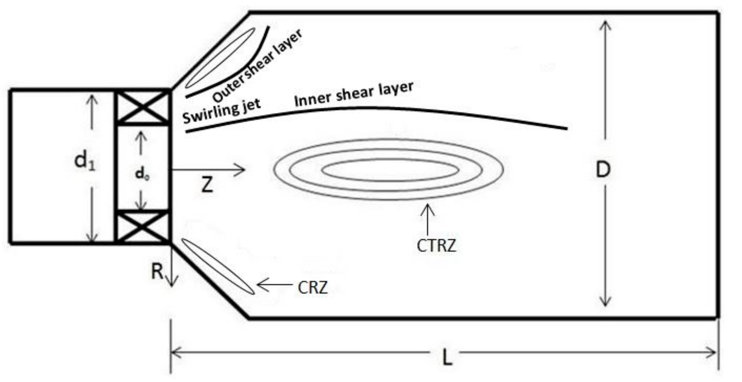
One of prominent characteristics of the swirl burner is its purposedly designed air supply method. Air flows enters the combustion chamber under the guide of curved blades which can generate recirculation zones around the head of the chamber. The recirculation zone consists of a Center Toroidal Recirculation Zone (CTRZ) and surrounding Corner Recirculation Zone (CRZ), as shown in
Figure 2. The recirculation zone can provide two basic functions, one is for anchoring the flame in the head of the chamber acting as a continuous source of ignition and another is for promoting mixing of fuel and air. As appropriate size and strength of recirculation zone are significantly important for achieving ideal combustion performance and stability, specifications of swirl burner must be optimized with adequate effort.
3.1. Flow Characteristics
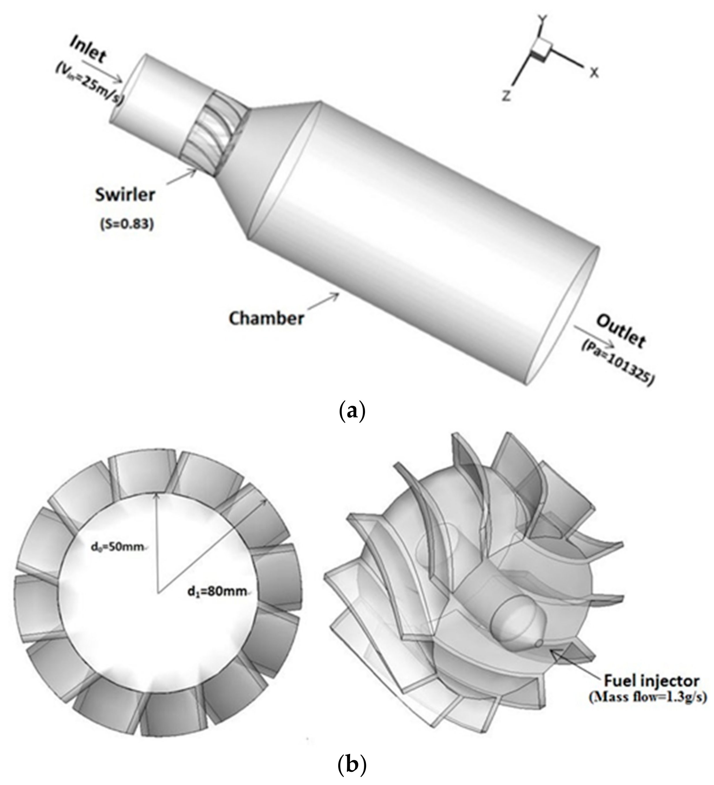
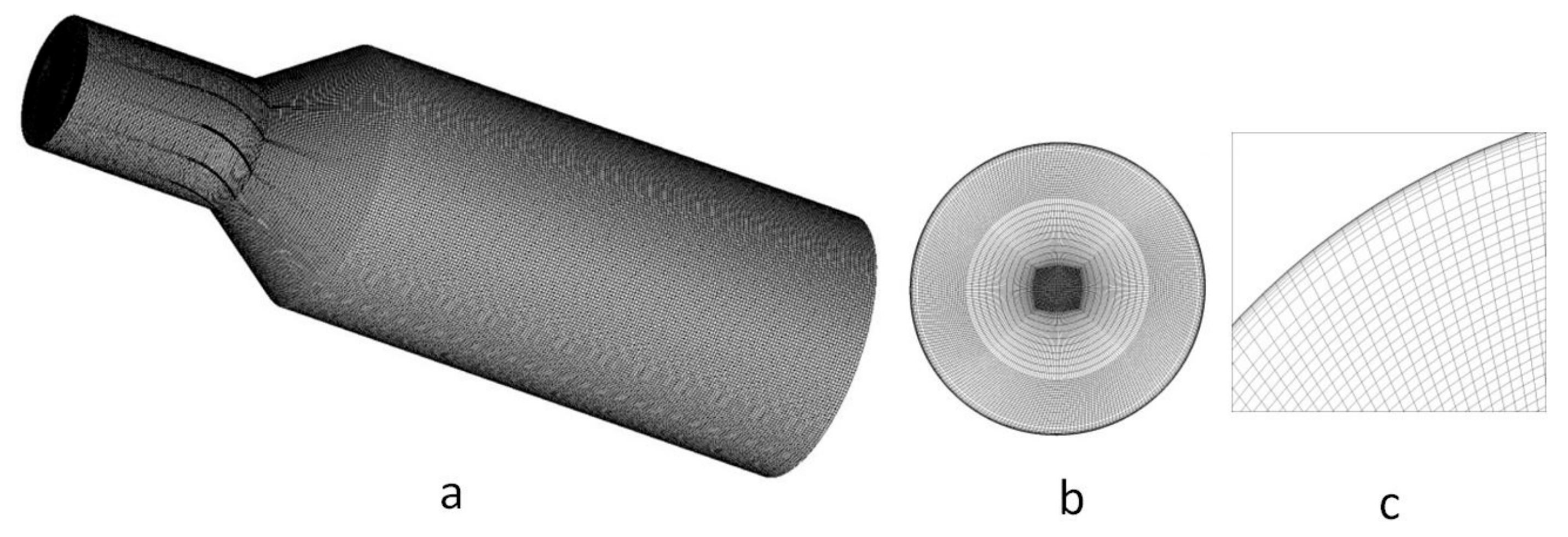
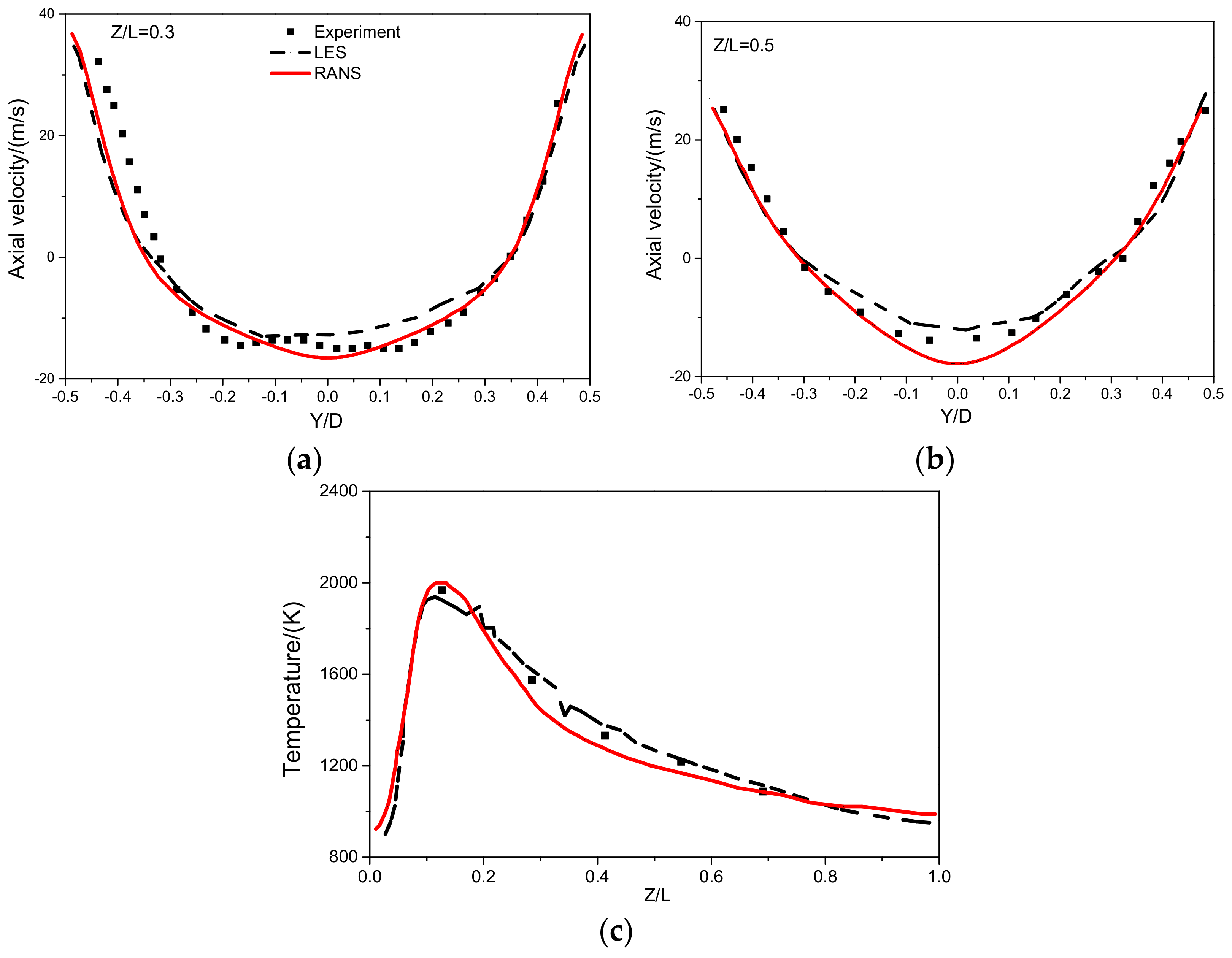
In order to investigate the flow field characteristic in a combustion chamber with swirl burner, velocity distributions have been simulated in detail and those results have been demonstrated along the chamber. The basic test conditions are listed in
Table 1. Three dimensional axial velocity, radial velocity and tangential velocity are expressed by U, V and W in the figures. At first, contours of axial velocity, produced by LES and RANS methods, respectively, were compared, as shown in
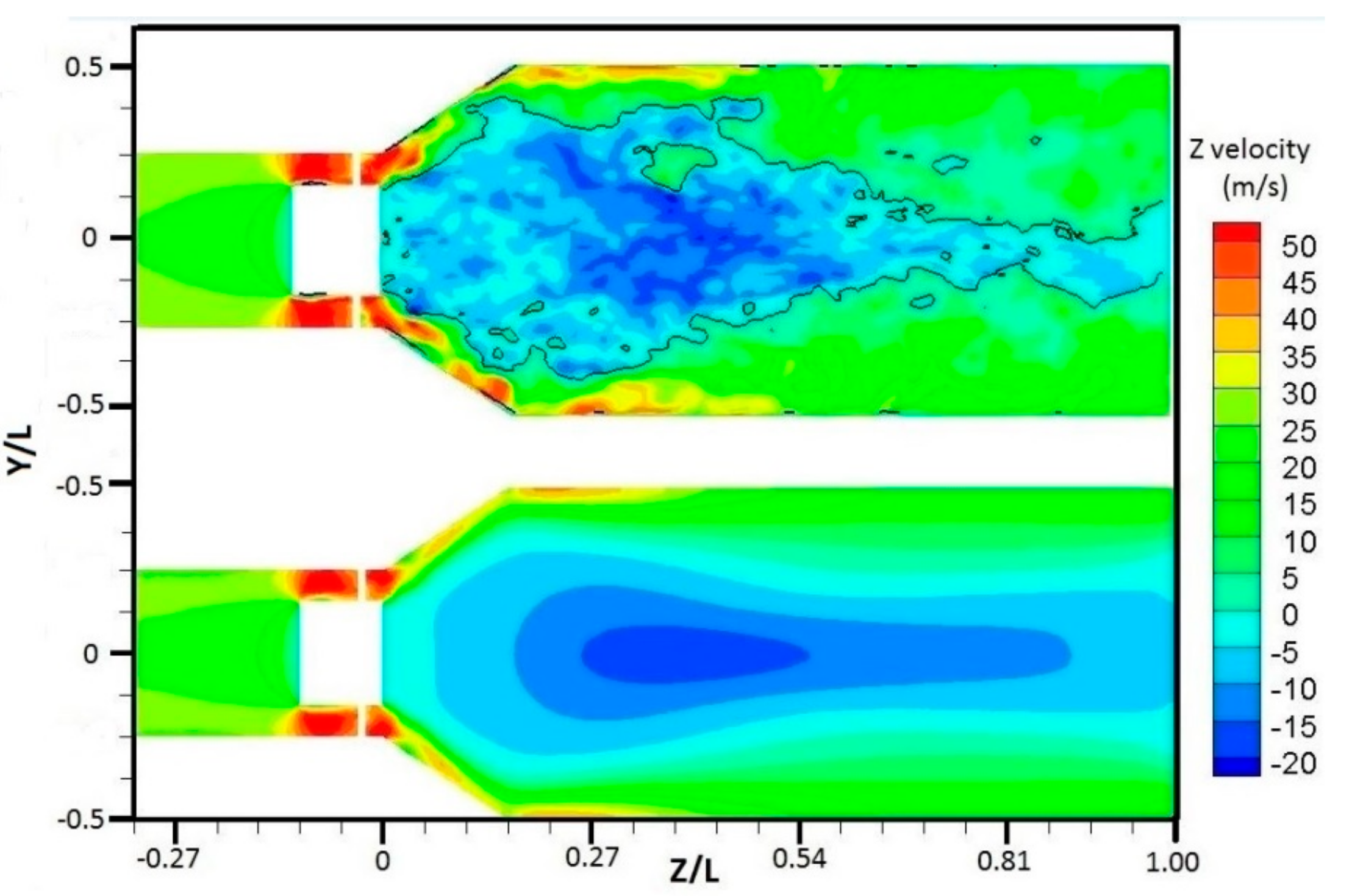
Figure 5. Compared to the RANS result, it can be seen that LES result can clearly demonstrate the detailed vortex structure. The black line which surround the central recirculation zone represents zero axial velocity. Under this tested high swirl number condition of swirler
S = 0.83, it is shown that the central recirculation zone extended for being close to the chamber outlet. The results shows that the maximum reverse velocity which is nearly 20 m/s is located at the upstream of the middle point of chamber. It may be due to too high velocity of annular jet flow which is injected into the chamber along the expanded wall, the corner recirculation zone is not obvious in this case.
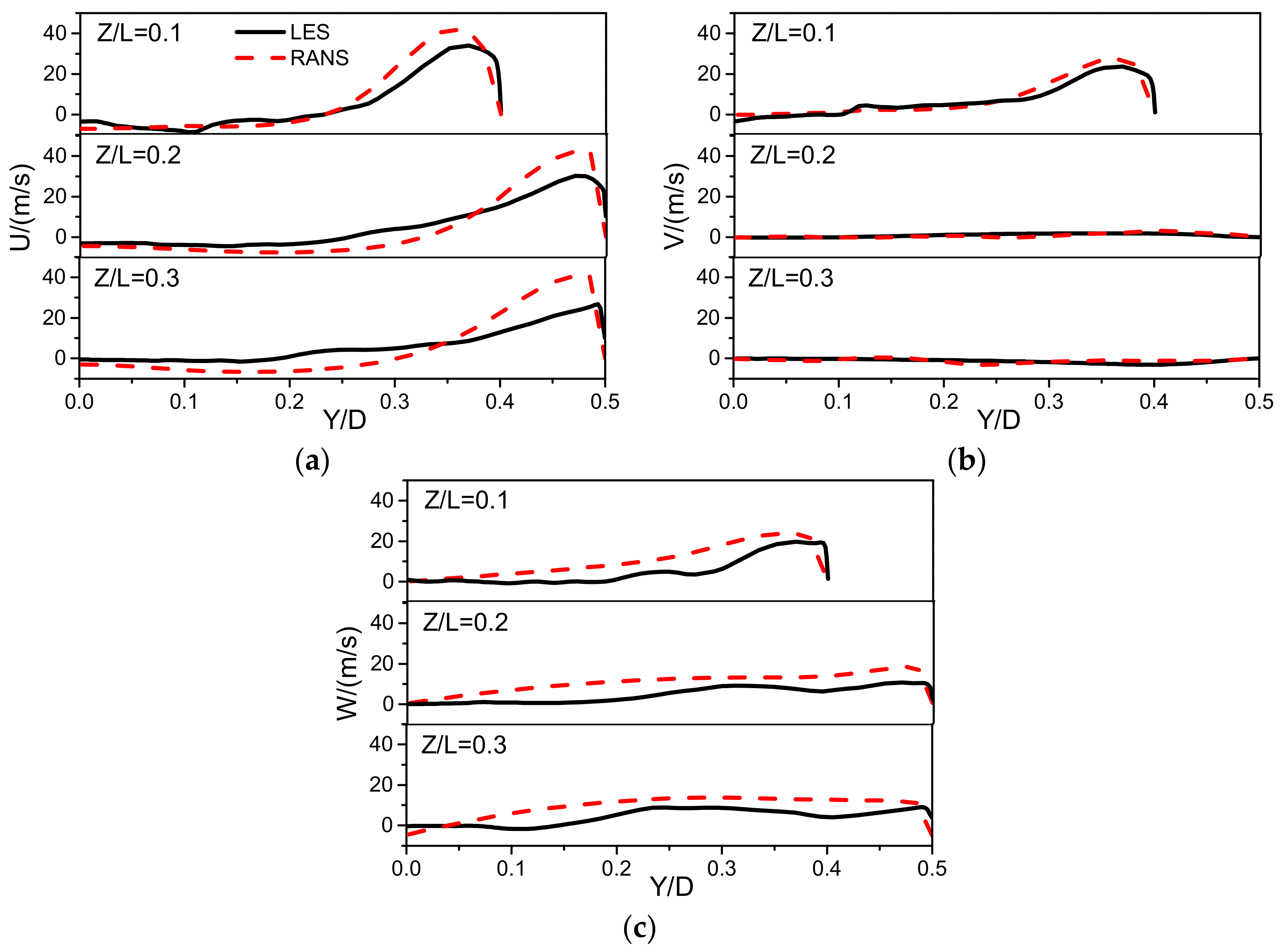
Figure 6 shows three velocity components of reactive flow field produced by LES and RANS, respectively. Only a half curve was expressed in those sections because of symmetrical geometry. It can be seen that axial velocities change gradually with the increase of distance away from the swirler exit. The radial position of the maximum axial velocities keeps moving to the combustor wall quickly with the increase of the axial distance from the swirler exit, and the maximum velocity value gradually becomes smaller. As shown from LES results, the overall maximum positive axial velocity is approximately 35 m/s which is located at around Z/L = 0.1. Negative axial velocity decreases gradually as flows move to downstream of chamber. This reverse flow nearly disappears after Z/L = 0.3. Then the axial velocity of recirculation zone becomes relatively flat.
As shown in
Figure 6, the radial mean velocity profiles are relatively flat, in particular after Z/L = 0.2. The maximum radial velocity appears around the outlet of the swirler. The mean radial velocity is almost zero in central part of the chamber since the main flow is in parallel to the axial direction. Compared to axial velocity and tangential velocity, radial velocity profiles have the best agreement between LES and RANS results. This may be due to limited effects of turbulence on radial velocities and the inadequacy of the LES in capturing the turbulence scales.
For swirl burners, mean tangential velocity can be the main velocity component for representing the most significant motion characteristics. Compared to the radial velocity profiles, the mean tangential velocities maintain a high value towards the downstream. It is indicated that the sustainable characteristics of high swirl flow and tangential velocity are closely related to the swirl number of the swirler. The velocity profiles of RANS results have higher values than LES which should be attributed to inaccuracy of its approximate processing method, especially around the region between the central line and the chamber wall. Similar distribution characteristics of the flow field have been found by experiments [
30]. Three dimensional velocities all have strong peaks at the upstream region. The highly peak radial velocity indicating a very expansion angle and all three velocity components peaks reduced significantly with the developments of flow to the downstream.
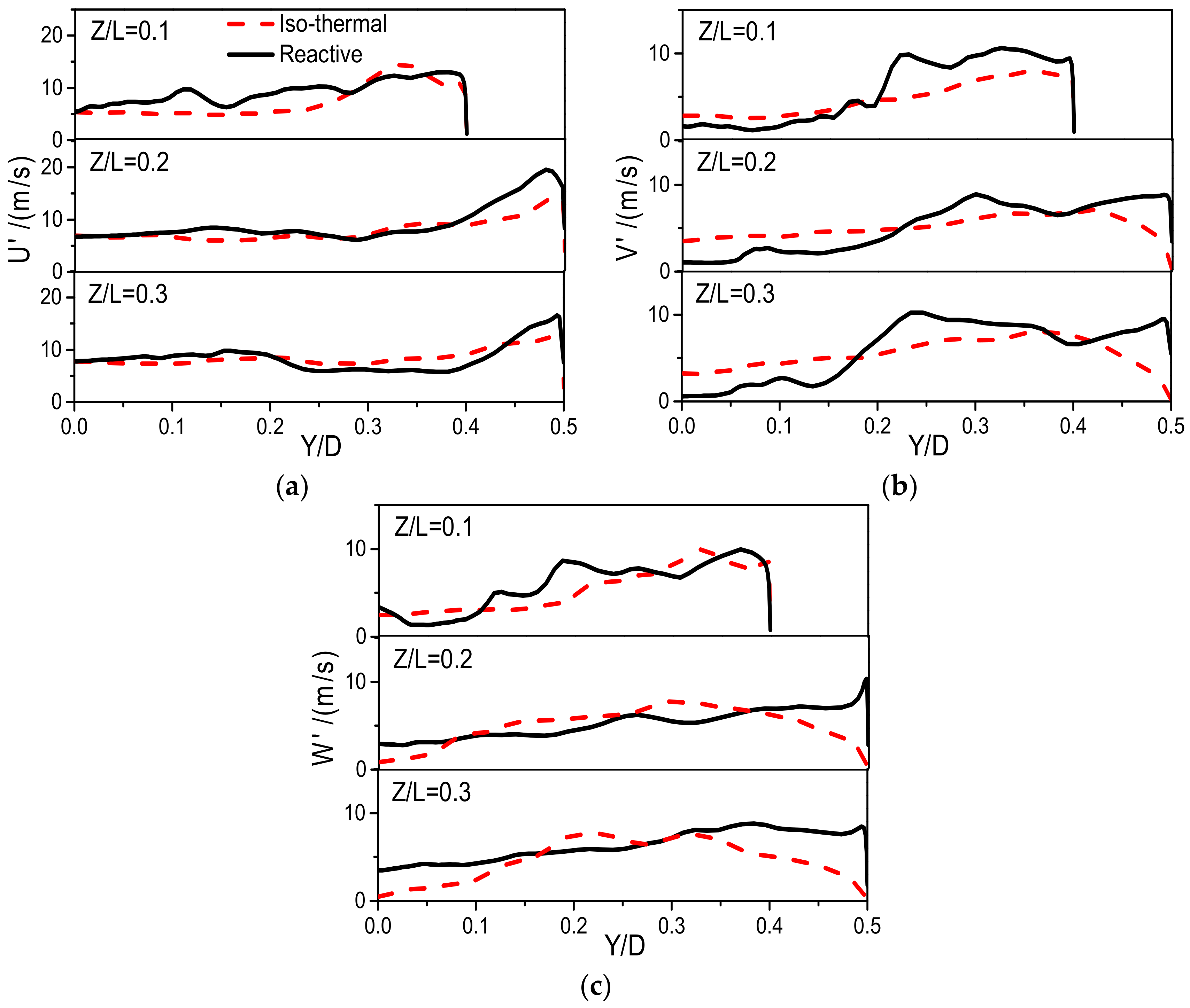
Figure 7 shows LES results for the Root Mean Square (RMS) of three velocity fluctuation components with a comparison between isothermal and reaction conditions. As lean combustion has been widely employed in gas turbines for environmental and efficiency concerns, an excess air factor of
with a kerosene mass flow of 1.3 g/s has been used for the simulation in this section.
As RMS value represents the turbulent fluctuations, it is expected the comparison can provide insight into effects of the combustion conditions on the turbulence characteristics. Under the isothermal condition, turbulent fluctuations of the axial velocity have a maximum U’ = 15 m/s which is at Z/L = 0.1 in the shear layer. However, the maximum RMS of axial velocity fluctuation of reactive flow appears at Z/L = 0.2 position where the main combustion zone should be. By comparing the isothermal and reactive results, it suggests that the combustion can obviously enhance the fluctuation of the turbulence. The value of U’ of combustion case decreases gradually towards to the downstream because of the turbulent dissipation.
On the contrary, the peak RMS value of tangential velocity has very limited change until the chamber outlet under this high swirl number condition. It is shown that the turbulent fluctuations decrease rapidly to zero around the chamber wall, and the fluid exhibits a strong laminar characteristic close to the wall. In the recirculation zone (from Y/D = −0.2 to Y/D = 0.2), the turbulent fluctuations of three velocity components are much smaller than those in the shear layer which is between the incoming stream and the recirculation zone as shown in
Figure 2. From Z/L = 0.1 to Z/L = 0.3, high RMS of the three components velocity fluctuations, in particular radial and tangential components, keep reduced and the peak profiles become wide. The smallest RMS of the velocity fluctuations appears around the combustion chamber central line, and also around the chamber wall. Meanwhile, RMS of the velocity fluctuations of radial and tangential components at the central line increase gradually towards to the downstream. This should be driven by the process of vortex core. Overall, the combustion is one of significant causes for resulting in unsteady flow field.
3.2. Combustion Processes and Temperature Distributions
In this section, the focus of simulation is on the investigation of combustion and emission characteristics of swirl burners. As in the last section, lean combustion was simulated with an excess air factor
and the kerosene mass flow of 1.3 g/s. The kerosene droplets with 60 m/s velocity under room temperature are injected into air flow which has a temperature of 450 K. The probability density function was used to describe the interaction physics of chemical reaction and turbulent flow. The chemical equilibrium assumption is used to calculate the probability density function table [
14,
28]. From initial simulation results, it shows that the combustion mainly occurs in the mixing region between the CTRZ reverse burned gas and the fresh fuel/air mixture.
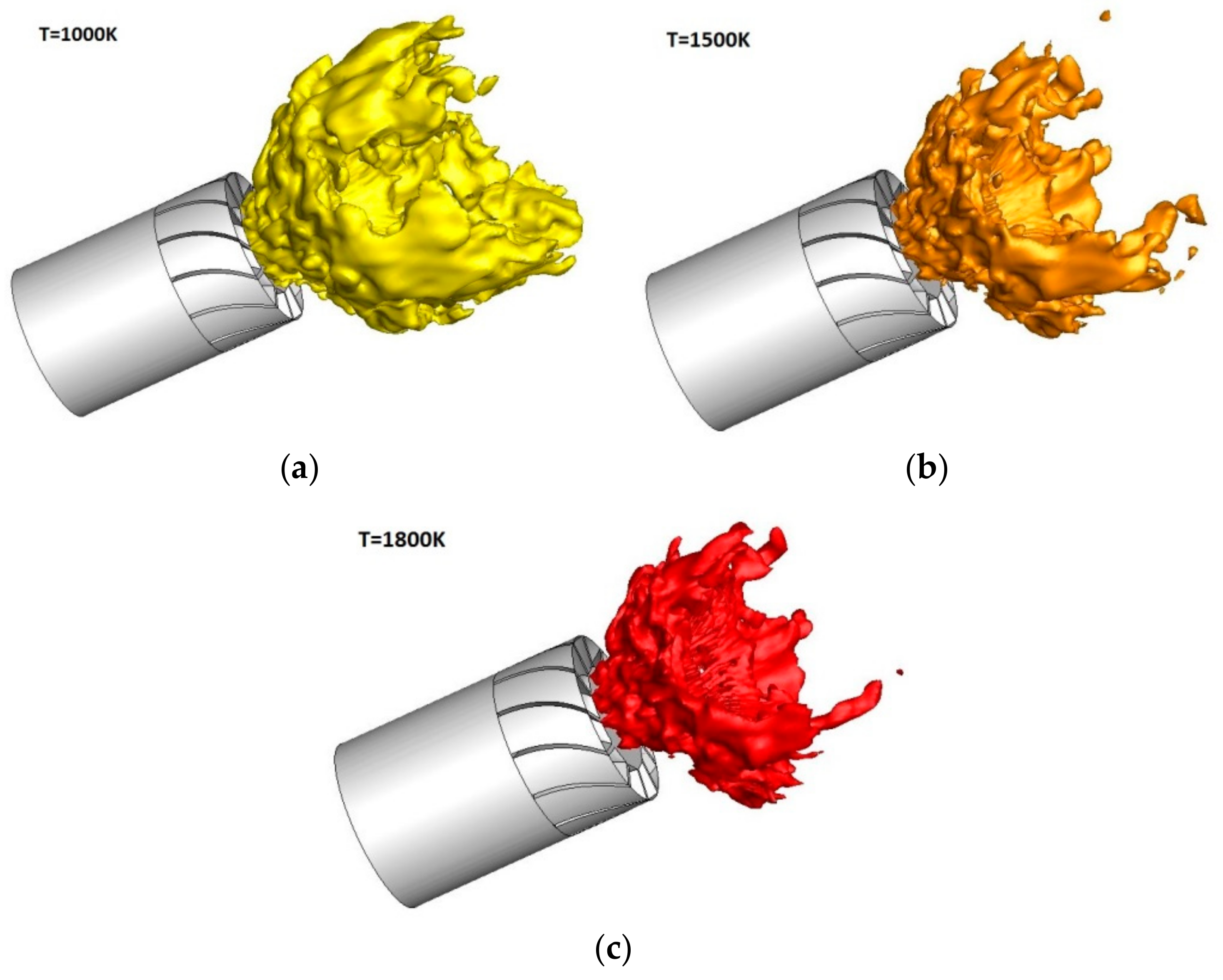
Figure 8 shows the contour plots of an instantaneous temperature field at 1000 K. The V shape flame is located near the chamber inlet position and it is a typical reaction zone structure that was created by the swirler for realizing stable combustion. In
Figure 8, it can be also seen that there is obvious wrinkling in the flame structure. This illustrates that the interaction of turbulence and the flame and the iso-surface is greatly distorted by vortices. Around the wrinkled region caused by vortex, there exists the main region of high temperature. Although those vortex structures will increase difficulty for controlling flame instability, they are beneficial for enhancing the mixing between fuel and gas, and improving the combustion and emissions of the burner [
31].
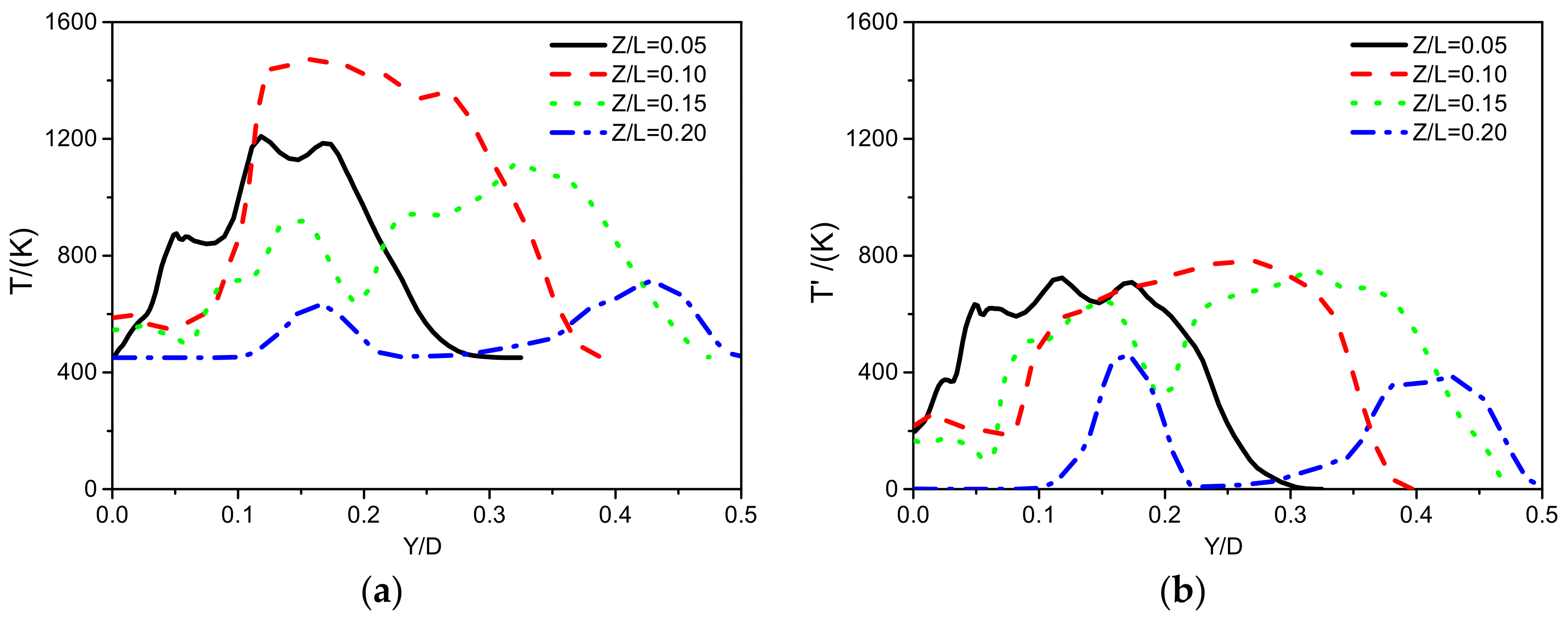
Figure 9 shows radial distributions of the mean temperature and RMS temperature at different positions. The maximum mean temperature which is just over 1400 K is located at the Z/L = 0.1 position. As the fuel is gradually consumed with the development of combustion to the downstream, the maximum temperature at each Z/L position keeps decreasing gradually towards to downstream, and the profile of temperature at each Z/L position becomes more flat, and from single peak to multiple peaks with the diffusion of flame because of the turbulent irregular movement. As shown in RMS temperature profiles, the peak value of temperature fluctuations occurs in the shear layer which is located between the inlet of fresh mixture and the recirculation zone as shown in
Figure 2. Downstream from the main reaction area, the temperature fluctuations decrease gradually. This demonstrates that the combustion is a main cause resulting in flow field instability.
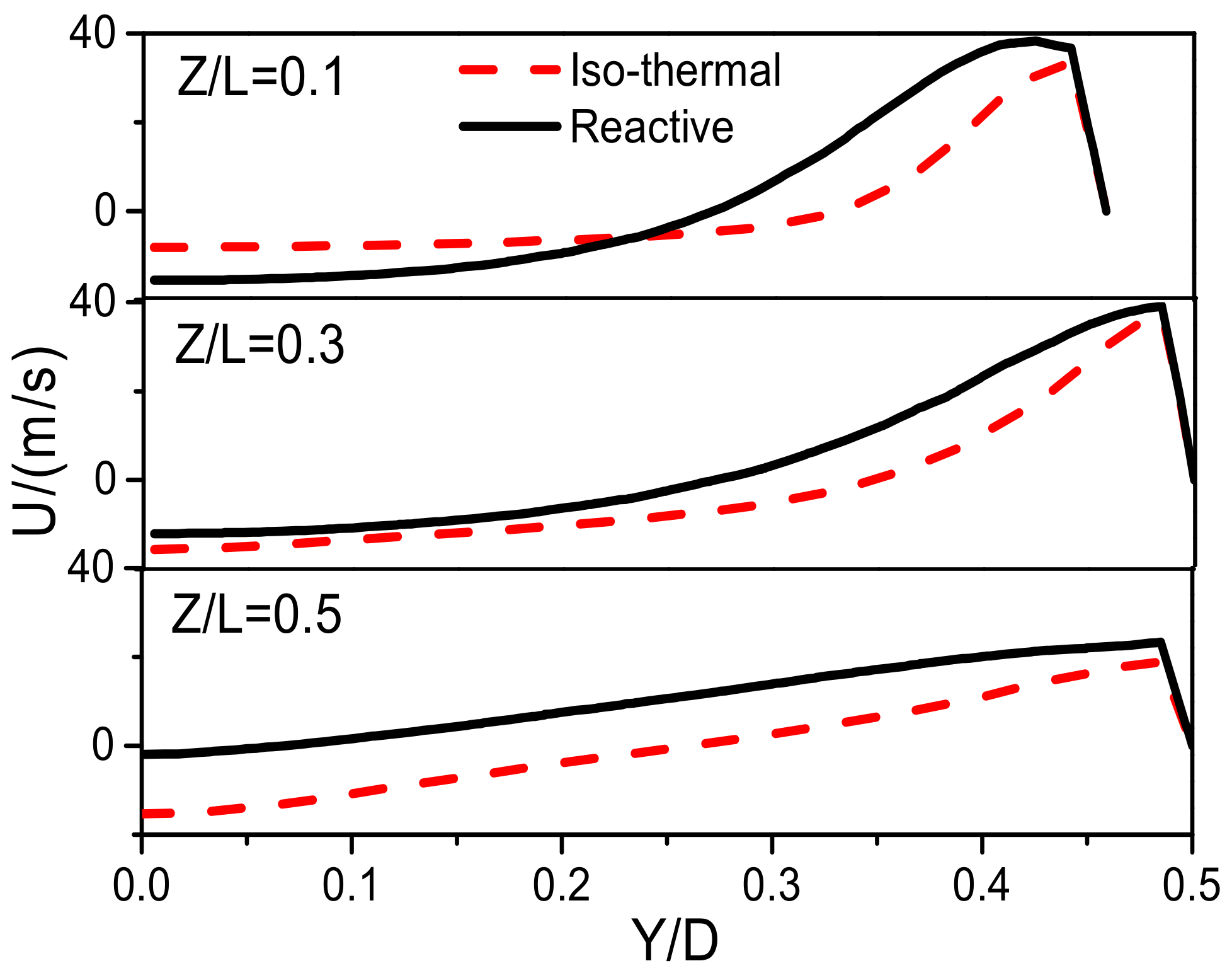
In order to examine effects of heat release on flow field, axial velocity profiles under the non-reacting and reacting conditions are compared at different position, as shown in
Figure 10. No doubt the combustion can significantly enhance the CTRZ, and both positive and negative axial velocities in the CTRZ are increased obviously under combustion condition. At the Z/L = 0.1 position, the reacting gas flow has the highest positive peak velocity around the shear layer and the highest negative velocity in the recirculation zone where the main combustion zone is. It is also found that the velocity decreases rapidly to zero near the wall due to the boundary layer. At Z/L = 0.3 position, the non-reacting axial velocity increases to the maximum value which represents the edge of the recirculation zone, but the negative velocity of the reacting gas becomes small compared to that at Z/L = 0.1 because of the high axial momentum. Down to Z/L = 0.5 position, the reacting gas negative axial velocity completely disappears and this should be the axial end of the recirculation zone. For non-reaction case, the reverse flow still exists at Z/L = 0.5. This suggests that the combustion condition results in the recirculation zone becoming smaller than in the non-reaction case, while the total axial momentum becomes bigger due to the combustion conditions. The peak velocities of both combustion and non-reaction decrease gradually because of the energy dissipation which is attributable to the heat transfer and the radiation of the chamber wall.
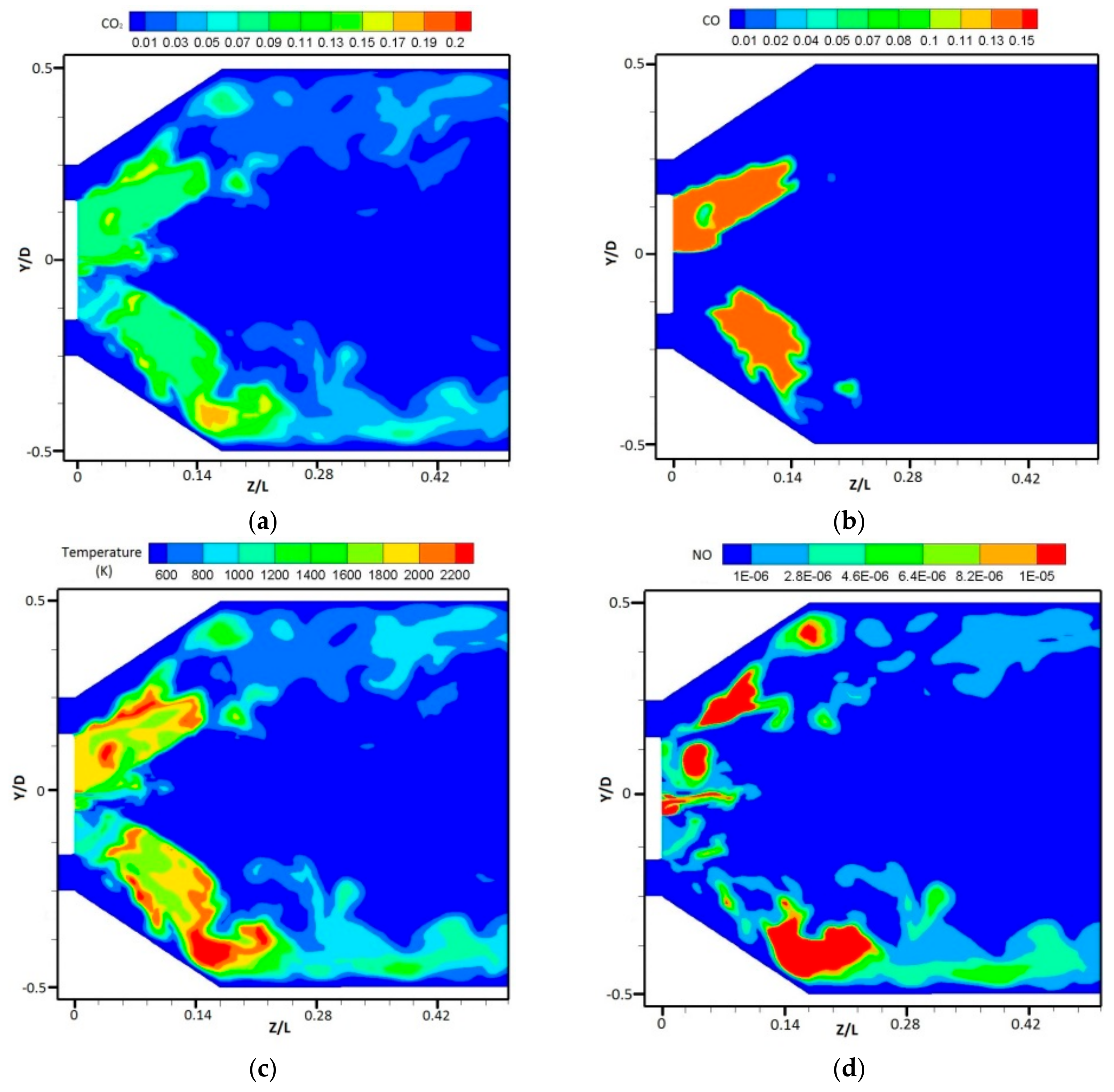
3.3. Species Concentration and Emissions
Under the combustion condition mentioned in last section, mass fractions of NO, CO and CO
2 are shown in
Figure 11. From the result, it can be seen that CO
2 is mainly created in the flame with the high concentration there, and disperses into the whole combustion chamber. CO mainly exists in the combustion zone with high concentration as a medium reaction species. Then most of the CO is further oxidized to CO
2. Therefore, it is obvious there is almost no CO existing after the combustion zone.
NO is mainly produced by the well-known thermal mechanism. As the combustion case is a lean burn with the maximum combustion temperature just over 1400 K, NO concentration is very low (less than 10 ppm), even in the combustion zone. Behind the combustion zone, NO is dispersed with a low concentration of less than 1 ppm.
3.4. Influence of Outlet Contraction
As all above investigations are based on a combustion chamber with open outlet, the influences of outlet contraction are studied in this section. The mean flow field varies with the difference of exit contraction ratios and the turbulent flow structure changes along the axial position of combustion chamber are investigated in this part. The investigation is mainly based on two outlet contraction designs. As demonstrated in
Table 2, the Cr (ratio of the outlet diameter to the combustion chamber main diameter) for the two cases are 1.0 and 0.563.
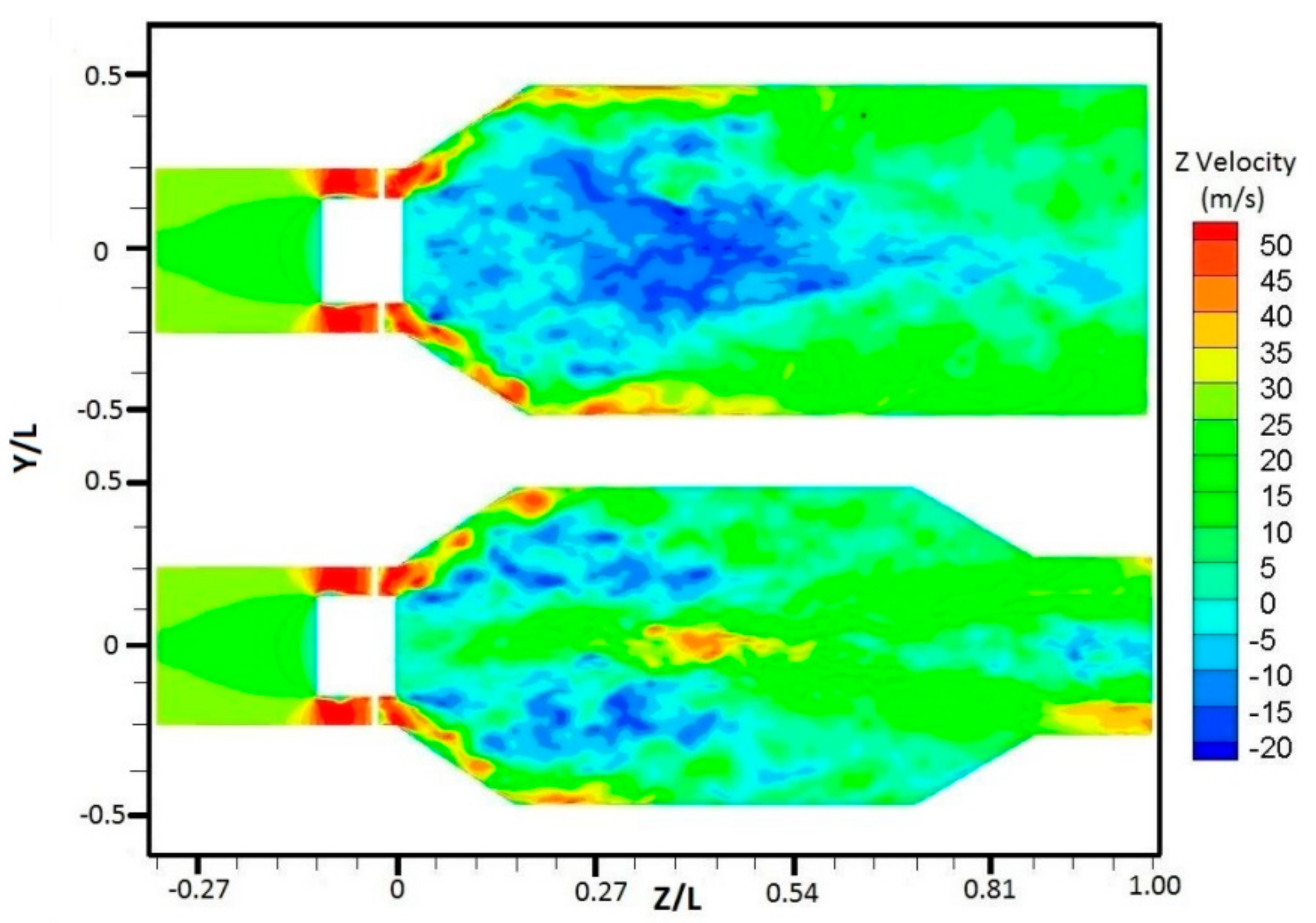
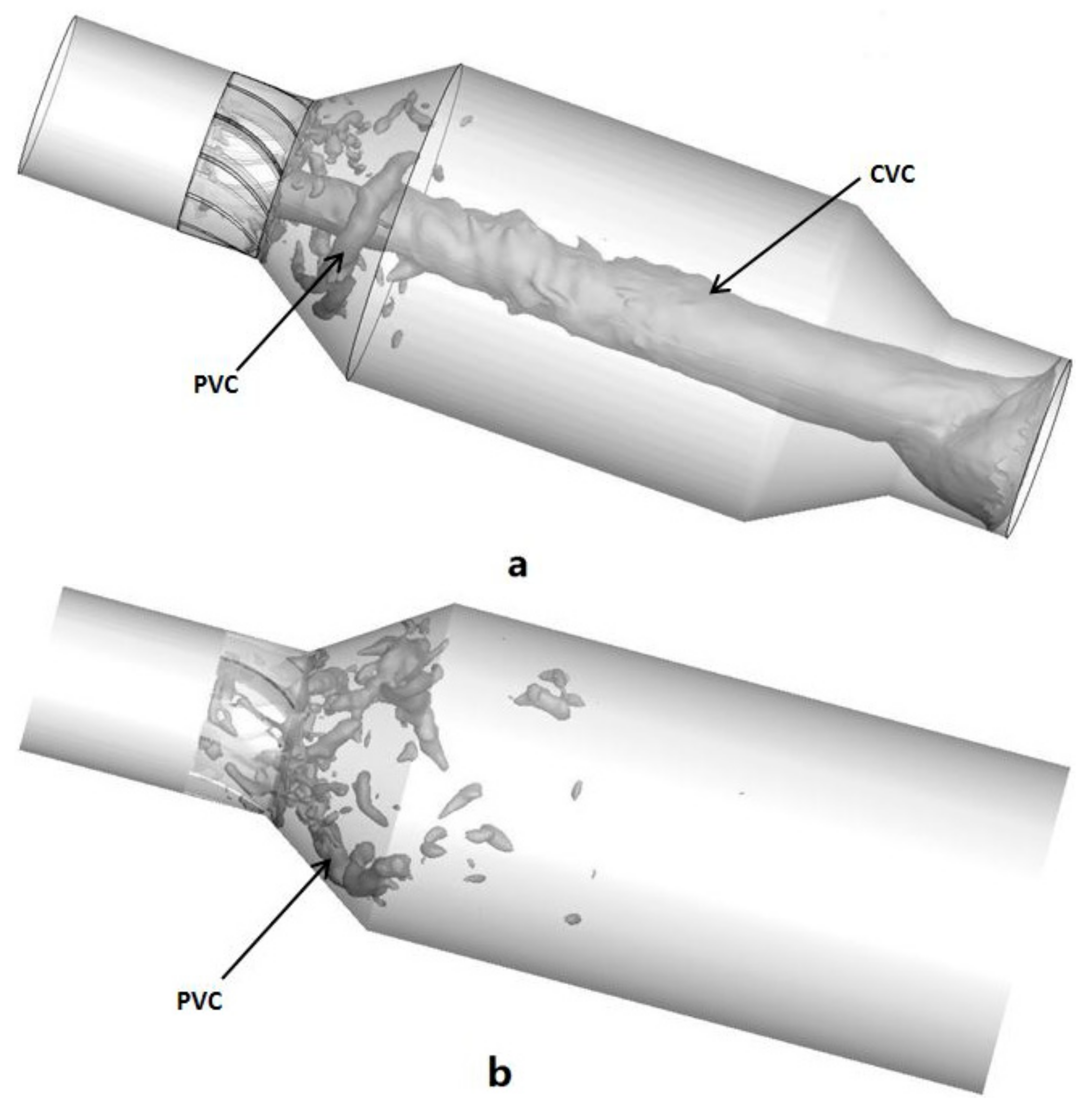
Figure 12 shows the axial velocity contour plots of Cr = 0.563 and Cr = 1.0. For Cr = 1.0 case, the central recirculation zone can penetrate into the whole straight chamber because of the large negative pressure condition that was created by the high swirling flow, but with the contraction of chamber outlet geometry of Cr = 0.563 case, the area of CTRZ decreases greatly and the axial velocity around the center-line changed from negative to positive. These results demonstrate that the flow field velocity distribution is affected by differences in the outlet structure under high swirl number conditions. In order to investigate the effect of the chamber outlet on vortex structure, the iso-surface instantaneous pressure method is used to display its three-dimensional structure because the vortex is generally created in a local low pressure region. Due to the existence of circumferential velocity, the pressure gradient would be generated in the radial direction. The local low pressure region will be generated when the flow field rotates. Many studies on the swirling flow have also proved that the instantaneous pressure iso-surface can be used to analyse the large eddy structure in the flow field effectively [
32]. As shown in
Figure 13, two separate structures are observed in chamber, that include PVC and CVC. The tornado-like CVC structure which can be observed in the case 2 is created by the rapid radial contraction of chamber which increase the angular velocity of flow field. The existence of such structures as a function of the outlet section geometry was experimentally proved by Escudier [
21].
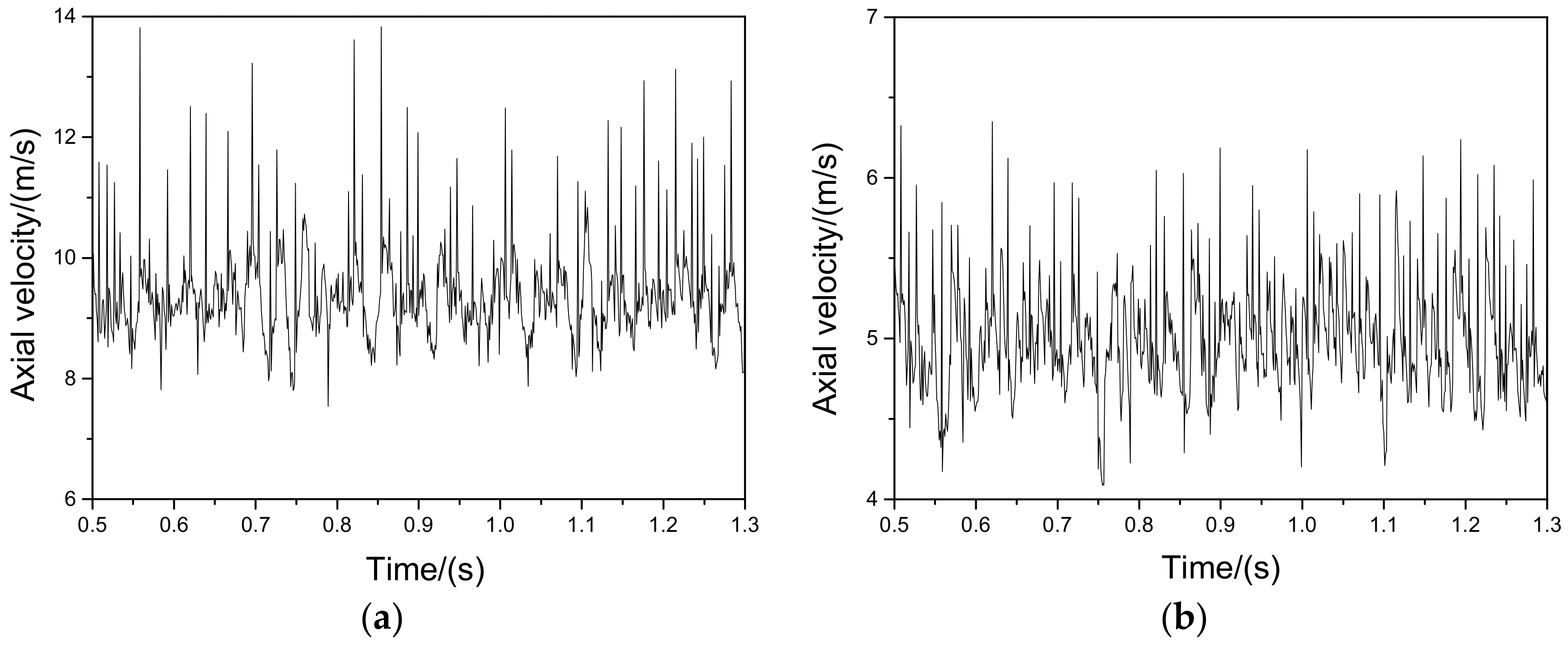
These vortices play an important role in turbulence mixing and transportation, but they are also the source of instability in the chamber, making it necessary to research the typical coherent structure and the highly unsteady phenomena caused by these vortexes. As the instability phenomenon caused by PVC structure has been widely studied, in this section the main concentration will be on the effects of the CVC structure on the instability of flow field. In Case 2, two positions were chosen as monitoring points, one point (0.0.200) is on the axis of chamber and 200 mm distant from the origin of coordinate, and another point (0.30.200) is 30 mm away from the axis. Time signals of the axial velocity were recorded at these two locations.
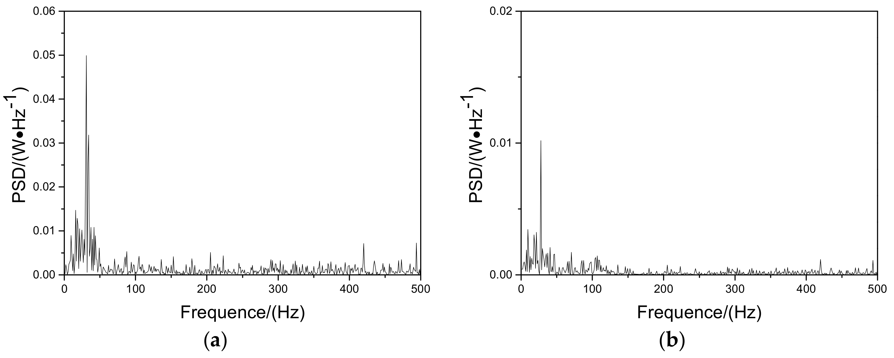
As shown in
Figure 14, the axial velocity fluctuation on the axis is relatively higher than the off-axis location. By analysing the frequencies of oscillation with Power Spectrum Density (PSD), it is demonstrated that a peak with the maximum amplitude for the spectrum on the axis is found at 31 Hz and at 27 Hz for the off-axis spectrum, as shown in
Figure 15. Obviously, the PSD peak is much stronger in the axis location than the off-axis point. This should be attributed to the motion of central vortex core around the center-line. This phenomenon shows that the CVC motion is one of the causes of the instability of the flow field.
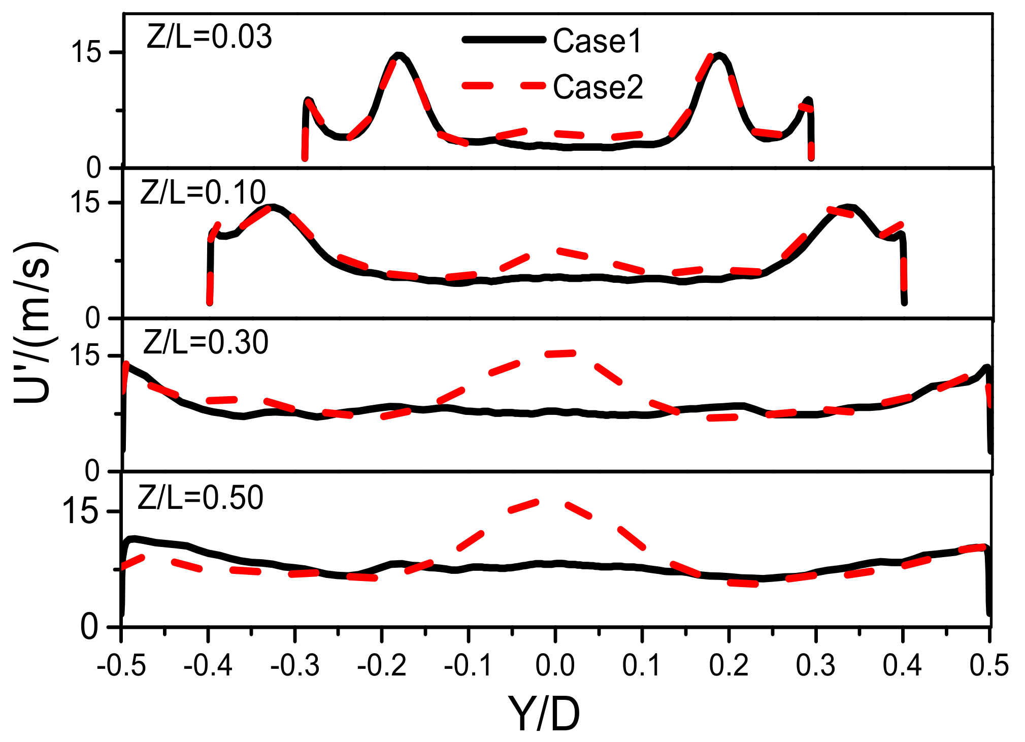
In
Figure 16, a comparison of RMS of the velocity fluctuations at different axial positions between Case 1 and Case 2 is presented. In Case 1, there is an obvious double peak velocity profile upstream and the maximum RMS of the velocity fluctuations is 15 m/s which located at the shear layer between the swirling jet and the central recirculation zone. The peak RMS levels at Z/L = 0.03 is caused by motion of PVC as shown in
Figure 10 and the peak value decreases gradually towards downstream. For Case 1, the RMS of the velocity fluctuations tends to flatten at Z/L = 0.5 and the maximum value is less than 10 m/s at the center-line due to the turbulent dissipation. On the contrary, there is a huge peak RMS of the velocity fluctuations appearing in center-line position in the result of Case 2 and the peak value is close to 18 m/s downstream. As this may be attributed to the motion of CVC, it may be assumed that main turbulent fluctuations at downstream are mainly driven by the tornado-like vortex because of the contraction of the chamber outlet, as shown in
Figure 13. For Case 2 with the outlet contraction, it can be observed that only those flows in the central field are affected by the outlet contraction structure. Those velocity distributions far from the central line of the chamber show very limited differences between Case 1 and Case 2. For all Z/L positions, it can be seen that the outlet contraction structure has a great influence on the downstream compared to the upstream field.


