Research on CO₂ Emission Reduction Mechanism of China’s Iron and Steel Industry under Various Emission Reduction Policies

Abstract

In this paper, a two-stage dynamic game model of China’s iron and steel industry is constructed. Carbon tax levy, product subsidy, carbon capture and sequestration (CCS) and other factors are included in the emission reduction mechanism. The effects of emissions reduction and the economic impact of China’s overall steel industry (and that of its six main regions) are investigated for the first time under different scenarios. As new findings, we report the following: (1) Not all factors declined. The overall social welfare, consumer surplus, output and emissions decrease with a gradual increase in the reduction target, whereas the carbon tax value, unit value of product subsidies and total subsidies show a rising trend; (2) A combination of multiple emissions reduction policies is more effective than a single policy. With the implementation of a combined policy, regional output polarization has eased; (3) Steel output does not exceed 950 million tons, far below the current peak. These results will help the industry to formulate reasonable emissions reduction and output targets. In short, in effort to eliminate industry poverty and to alleviate overcapacity, the industry should not only adopt the various coordinated reduction policies, but also fully consider regional differences and reduction needs.

1. Introduction

China has established the world’s most complete iron and steel industry chain system, which provides most the iron and steel materials for the national economy [1]. In 2011, the output was 850 million tons and in 2015 it equaled 1.02 billion tons, after reaching a historical peak of 1.046 billion tons in 2014. The domestic market share of steel is over 99%, effectively satisfying national economic and social development.

Even so, the iron and steel industry faces non-neglected problems, especially the overcapacity. In 2015, China’s steel production capacity reached 1.13 billion tons, far exceeding its 1.02 billion tons of actual production. Steel production capacity has gradually shifted from regional, structural surplus to absolute excess. The concentration degree has ceased to rise, and the first 10 iron and steel enterprises’ concentration degree fell from 49% in 2010 to 34% of 2015. Although energy consumption and pollutant emissions of per ton steel are decreasing year over year, these changes cannot offset the increase in energy consumption and total pollutants caused by the excessive steel output. In particular, in the Beijing-Tianjin-Hebei region and the Yangtze River delta, the environmental carrying capacity has reached its limit. A large area of haze has spurred significant environmental pressure and negative public opinion, forcing the government to enact more stringent industry policies and environmental protection measures in the iron and steel industry.

Therefore, the prediction of a reasonable production interval and calculation of the emissions level can provide data and reference support for eliminating excess capacity and formulating CO₂ emissions reduction targets. This is one of the starting points and importance of this paper.

In addition, in the future, sole dependence on technology innovation will no longer fulfill CO₂ emissions reduction targets, and this will also increase enterprises’ investment. Therefore reasonable carbon tax policies and government subsidies are imperative. In addition, to better control emissions reduction, carbon capture and sequestration (CCS) represents another way to reduce CO₂ on a large-scale. Over the next 15 to 30 years, China’s steel industry CCS demonstration projects will be planned and put into production, so large-scale investment in CCS projects also concerns to the enterprise and government. Therefore, reasonable reduction technologies and system policies can provide a foundation for the subsequent development of regional emissions reduction policies and economic impact assessment, hence the second aim of this paper.

The remainder of this paper is organized as follows: Section 2 provides a literature review focusing on the carbon tax levy system and production subsidies mechanism research. Section 3 introduces the two-stage game theory modeling, policy assumptions and data sources. In Section 4, based on accounting data and statistical analysis, we present and discuss our results in detail. Section 5 provides conclusions and policy recommendations for China’s iron and steel industry.

2. Literature Review

Many economic scholars have studied CO₂ reduction policies, including carbon tax, carbon trading, and carbon sink. Most carbon tax levy systems and production subsidies have focused on the general equilibrium model. By setting different tax rate and output subsidy return conditions, the emissions reduction effect and impact on the economy have been analyzed using the CGE model (computable general equilibrium model, typically composed of a set of equations to describe supply, demand and market relationships). Other academic models have been employed as well.

In the field of CO₂ reduction, Jorgenson et al. [2,3] used the CGE model in pioneering research. Manne et al. [4] introduced a carbon tax module via the MERGE model, in which they calculated and analyzed the differences in cutting emissions costs in different regions of the world. Jorgenson and Wilcoxen [5] predicted the effect of the energy tax by using a CGE model. Zhang [6] used the CGE model to examine the economic implications of carbon abatement for the Chinese economy in the first systematic and comprehensive attempt. Later Zhai and Li [7], Xie et al. [8,9] conducted the similar study using the CGE model as well.

Since the beginning of the 21st century, the CGE model has been improved and developed. This model has been applied to many countries, sectors and more policy scenarios. For example, Kemferthe and Welsch [10] analyzed the economic effects of government carbon tax policy using a dynamic CGE model to discuss different elasticities and tax-returning mechanisms between energy and capital, energy and labor. Wendner [11] used a general equilibrium model to analyze the carbon tax impact on the Austrian economy. Van Heerden et al. [12] found that the environment tax can be given back to the industrial sector by reducing labor and capital taxes directly using a CGE model. Abrell [13] analyzed the use of market-based emissions regulation instruments to address CO₂ emissions in transportation. Benavides et al. [14] examined the economy-wide implications of a carbon tax applied in the Chilean electricity generation sector via both an energy sectorial model and a dynamic stochastic general equilibrium model. Yahoo and Othman [15] evaluated the economy-wide impacts of implementing two different types of CO₂ emissions abatement policies in Malaysia using market-based (i.e., carbon tax) and command-and-control mechanism (i.e., sectoral emissions standards). These papers were directed at a particular country or sector, with a specific tax or subsidy value. By calculating the results using CGE models, researchers can gauge the economic and environmental response.

Using the input-output table published by the Chinese Statistical Department, scholars have analyzed the impact in China of imposing an energy tax and subsidy on the economy, energy, environment and production sectors. This research has been extended to provinces and sectors.

Liang et al. [16] examined how to reduce carbon tax on the export of energy-intensive industry international competitiveness by a CGE model. They suggested offering a tax break on energy-intensive, labor-intensive export industries, and implementing a carbon tax return for other industries Yang et al. [17] used a CGE model to quantitatively simulate the impact of energy tax scenarios. They found that an energy tax can help to minimize the CO₂ and SO₂ emissions, with increasing marginal emissions reduction costs. Wu et al. [18] developed the China regional dynamic general equilibrium model and analyzed the marginal cost curve between various provinces and cities from 2007 to 2020, then discussed carbon emissions trading and carbon tax policy choices. Xu and Zhang [19] applied a multi-sectoral dynamic CGE model to analyze the impacts of a carbon tax on China’s economy and carbon intensity at the rate of 40 yuan/t without tax relief as a baseline scenario. They also compared the change trends of carbon intensity and the proportion of non-fossil energy in primary energy consumption from the perspective of achieving the emissions reduction targets in 2020 and 2030. Chen et al. [20] established an energy CGE model for Guangdong Province, and simulated the energy-saving and emissions reduction effects from the enactment of an energy tax or carbon tax at various tax rates, they also analyzed the mitigation effects on an economic system given various tax refund plans. Ling et al. [21] built a multi-sectoral dynamic CGE model with a coal resource tax module, to study the general impacts of such reform policy on the Chinese economy and environment. However, due to specific parameter values and assumptions, along with the rapid development of China’s economy, these studies’ results do not necessarily correspond to the actual situation. Moreover, the social accounting matrix (SAM) requirement is higher and this data is not published every year.

There have also been many papers on environmental regulations using game theoretic approaches. Scholars have applied game theory to the study of carbon tax levy and subsidy mechanism. Extant literatures have focused primarily on constructing a two-stage game model to establish the relationship between the government and enterprise, and between different enterprises. In particular, scholars have studied the optimal level of emissions and the optimal output of subsidy mechanisms.

Much of the early research on environmental regulations using game theoretic approach focused on permits, standards and technological innovation. Montero [22] and Bruneau [23] compared the incentives to invest in environmental research and development (R&D) offered by four policy instruments—emissions standards, performance standards, tradeable permits, and auctioned permits- and found the relationship between abatement, innovation, and the production process itself to be critical to a sound understanding of these incentives. Then product differentiation, countervailing incentives and other market-based instruments were incorporated into the theory, such as by Requate [24,25], Puller [26] and Poyago-Theotoky [27,28].

In subsequent studies, scholars have applied the game theory approach to environmental regulations and reduction mechanisms. Youssef et al. [29], Ouchida and Goto [30], and Moner-Colonques and Rubio [31] looked into the society economic levels under different environmental policies. Demailly and Quirion [32] quantified the impact of the European Emission Trading Scheme on two dimensions of competitiveness, production and profitability, for the iron and steel industry. Under a mixed market structure, Cato [33] proposed an emissions reduction mechanism based on a subsidy reduction, and demonstrated that the mechanism could achieve an optimal social result. Eyland and Zaccour [34] looked at the optimization of two different governments and their respective firms. Parametric values inside the set [0, 1) were used to represent the possible extents of the border tax adjustment (BTA) depending on both countries’ respective environmental policies allowing countries to have different carbon policies. To examine the applicability of the “Pigouvian tax” in China’s present low-carbon economy, Ouchida and Goto [35] concluded that social welfare under a time-consistent emissions tax (emissions subsidy) policy was always welfare-enhancing rather than laissez-faire. McDonald and Poyago-Theotoky [36] found a counterintuitive positive relationship between R&D input spillovers and emissions taxes and a U-shaped relationship between the optimal emissions tax and R&D spillover in the d’Aspremont and Jacquemin (AJ henceforth) model. Lambertini et al. [37] explored the relationship between competition and innovation when R&D investment attempts to reduce pollutant emissions. They have uncovered an inverted U-shaped relationship between “green” innovation and competition. It can be said that the application of game theory abroad has been more mature and systematic.

In China, there is also much research on environmental regulations from a game theory approach. Li et al. [38] proposed a two-stage dynamic game model comprising two sub-games involving a government-firm and firm-firm relationship. They also investigated the second-best emissions tax and its revenues refunding scheme based on an output subsidy with exogenous abatement target. Li et al. [39] constructed a two-stage dynamic game model based on two representative iron and steel firms (eastern and western) to examine the effects of a uniform or discriminated emissions tax levied by the central government on abatement costs, social economic welfare and the firms’ competitiveness. Zhang [40] built a three-stage game model between the government and enterprises to analyze the feasibility and mode selection of carbon tax policy. In the process of supply chain low-carbonization, a three-stage game model was constructed by Li et al. [41] between the government and enterprises by considering carbon tax as one regulation mode. Qiao et al. [42] made the first attempt to use non-cooperation game theory to study airlines’ carbon tax strategies in the EU. Xu et al. [43] studied joint production and pricing problem in a manufacturing firm with multiple products under cap-and-trade and carbon tax regulations, and compared the effects of the two regulations on the total carbon emissions. However, because China has not yet implemented an emissions trading mechanism, carbon tax mechanism, or other emissions reduction policies, research can only establish models and make scenario assumptions.

Extant literature shows that the research on reduction mechanism is comparatively developed. Firstly, the CGE model and game theory can provide policy references for emissions reduction. Nevertheless, the CGE model used to study tax reduction mechanisms generally focuses on the specific tax rate and output subsidy, to identify the corresponding reduction. Game theory seeks to assess the optimal emissions level and output subsidy mechanism; therefore, this method is more suitable for the government to observe the economic and environmental changes between countries and regions when formulating a certain emissions reduction policy.

Secondly, we found that research has traditionally focused on national-level and overall sectors (e.g., industry, service industry, agriculture), whereas research on the provincial level and a single industry department is limited. Yet the steel industry is a foundational component of the China’s national economy and one of the industrial sectors with the greatest CO₂ emissions, which undertakes important emissions reduction tasks to control the nation’s greenhouse gases.

Thirdly, the literature highlights models, but empirical analysis is lacking. The basic parameters of empirical analysis (especially based on enterprises) are usually derived from existing data from developed countries. In developing countries like China, there are significant regional differences and regional economic development imbalances; thus, some areas’ parameters and data, including those of the iron industry, need to be supplemented.

In addition, with the continuous development of China’s economy and the world’s constant attention to environmental problems, the pressure around emissions reduction will only continue to increase. A separate carbon tax or product subsidy policy would not meet the country’s economic development and emissions reduction level needs. Projects such as CCS, carbon sinks and other significant CO₂ emissions reductions methods will likely be incorporated into the entire reduction system. Therefore, game theory warrants attention in this respect.

In conclusion, a reasonable reduction policy is the primary focus of this paper. The paper organizes energy, environment and economic data from the six main areas’ of the iron and steel industry in China. Combined with the corresponding long-term plan issued by the government, we consider and integrate the carbon tax, production subsidies, CCS, and external loss of CO₂ into the emissions reduction mechanism to build a two-stage dynamic game model. Then, based on different periods of the steel industry’s carbon emissions with decreased demand, we discuss the six main areas’ market game behavior under different reduction targets, and investigate the differential effects of emissions reduction scenarios and their economic impacts on the iron and steel industry.

3. Methods

3.1. Notations and Explanations

According to the regional division of China, China is divided into six regions: North China (i.e., Beijing, Tianjin, Hebei, Shanxi, and Inner Mongolia), Northeast China (i.e., Liaoning, Jilin, and Heilongjiang), East China (i.e., Shanghai, Jiangsu, Zhejiang, Anhui, Fujian, Jiangxi, and Shandong), South Central China (i.e., Henan, Hubei, Hunan, Guangdong, Guangxi, and Hainan), Southwest China (i.e., Chongqing, Sichuan, Guizhou, Yunnan, and Tibet), Northwest China (i.e., Shanxi, Gansu, Qinghai, Ningxia, and Xinjiang). In this paper, regions are presented by subscripts: 1 represents North China, 2 represents Northeast China, and so on.

The main research focus of this paper includes the government and the above six regions, the regional steel industry data is regarded as a steel enterprise entity). The government emissions reduction policy is a double game problem. Firstly, there is a decomposition game between the government and regional enterprises: government stipulates the emissions reduction target for a certain period, after which the regional enterprises should determine their respective reduction ranges according to their own cost curves. Secondly, there is a game of product output between the six regions, and the different targets of the regional enterprises will affect their respective output levels and market competitiveness.

Therefore, the resultant game order is as follows: in the first stage, the government set corresponding reduction targets and reduction policies (e.g., carbon tax, product subsidies, CCS, independent or mixed); in the second stage, on the premise of guaranteeing profit maximization, the regional enterprises choose their respective reduction targets and output levels simultaneously. Based on this idea, this paper adopts the inverse method to solve the two-stage game problem. The notations used in this paper and their explanations are presented in

Table 1. Notations and explanations used in this paper.

Notations	Explanations
Q	Steel production
P	The price of steel
α	The constant of the market inverse demand curve
β	The primary coefficient of the market inverse demand curve
qi	Steel production of region i
e	The national CO2 emission intensity of per ton steel in 2010
e2015,i	The region i CO2 emission intensity of per ton steel in 2015
ei	The region i CO2 emission intensity of per ton steel at some stage
ri	The decline range of CO2 emission intensity of per ton steel in region i at some stage
R	The decline target of national CO2 emission intensity of per ton steel at some stage
MAC	Marginal abatement cost curve in iron and steel industry
ai	The primary coefficient of steel industry’s MAC in region i
bi	The quadratic coefficient of steel industry’s MAC in region i
Ci	The cost function of steel industry in region i
C0,i	The production cost of steel industry in region i
T	The total carbon tax
t	The unit value of carbon tax
W	Social welfare function
CS	Consumer surplus
PS	Producer surplus
θ	The external loss parameter of CO2
η	The production subsidies
m	The CO2 emission reduced by CCS demonstration project
A	The primary coefficient of CCS demonstration project cost curve
B	The constant of CCS demonstration project cost curve
πi	The profit function of steel industry in region i
E	The total CO2 emissions in iron and steel industry
S	The total subsidy
M	The total cost of CCS demonstration project

.

It is assumed that each regional enterprise produces homogeneous products and compete for production in the product market. There is no regional variability and the prices of steel are the same. The market reverse demand curve of the enterprise is P(Q). This paper describes the relationship between product price and demand using a linear combination, and P′(Q) < 0, where P indicates price, Q is total output, and $Q={\displaystyle \sum }_{i=1}^6{q}_i$. At the same time, the paper assumes that in the future equilibrium market, production and consumption are equal. The production cost of the enterprise is different, while the marginal emissions reduction cost is incorporated into the cost function, namely $C_i\left(r_i,q_i\right)$, where $e_i=e_{2015,i}\left(1-r_i\right)$. It is assumed that the cost function satisfies $\underset{r_i=1}{\lim }{C}_i\left(r_i,q_i\right)=+\infty$, $\partial C_i/\partial q_i>0,{\partial }^2{C}_i/\partial q_i{}^2>0,\partial C_i/\partial r_i>0,{\partial }^2{C}_i/\partial r_i{}^2>0$. D(E) represents an external macro loss to the environment caused by CO₂ emissions, $D\left(E\right)=\theta \left(E\right)=\theta {\displaystyle \sum }_{i=1}^6{e}_i{q}_i$. In addition, because the CCS cost curve is still in the valuation stage, and is directly related to the amount of CO₂ trapped in the transport storage, the curve approximation is proposed to synthesize the linear relation, M = am + b.

3.2. Modeling

3.2.1. Scenario Analysis

In this section, we discuss three scenarios due to policy uncertainties:

Case 1: Only carbon tax scenario

At present, carbon taxes are likely to be the only policy tool for reducing emissions targets, due to policy and technological constraints.

Case 2: Mixed scenario, Carbon tax and subsidy

With the gradual increase in emission reduction targets, carbon tax reduction will seriously compress producers’ profit, so subsidies based on product output may increase producers’ enthusiasm and ability to produce. This paper assumes that subsidies are derived from carbon taxes. More specifically the carbon tax levy will be partially or entirely returned to the producer in the form of subsidies.

Case 3: Mixed scenario, Carbon tax, subsidy, and CCS

As emissions reduction targets continue to grow, carbon tax and subsidies may not fulfill the criteria for reducing emissions. At the same time, with advancing technology and increasing tax pressure, CCS will be employed over the mid- and long-term as a means of large-scale CO₂ emission reduction. A mix of reduction policies will help achieve the CO₂ emissions reduction target more easily. This paper assumes that the subsidy comes from carbon tax, and CCS demonstration project is funded through government investment.

3.2.2. Two-Stage Dynamic Game Model

In the second phase of the game, the government sets emissions reduction targets and reduction policies. Regional enterprises choose their own production and reduction targets, and the profit function under different cases are as follows:

$${\pi }_{case1,i}=P\left(Q\right)q_i-C_i{q}_i-T_i=\left(\alpha -\beta Q\right)q_i-q_i(C_{0,i}+{{\displaystyle {\int }_0^{r_i}MAC}}_i\left(r\right)dr)-t{e}_i{q}_i$$

(1)

$${\pi }_{case2,i}=P\left(Q\right)q_i-C_i{q}_i-T_i+S_i=\left(\alpha -\beta Q\right)q_i-q_i(C_{0,i}+{{\displaystyle {\int }_0^{r_i}MAC}}_i\left(r\right)dr)-t{e}_i{q}_i+\eta q_i$$

(2)

$${\pi }_{case3,i}=P\left(Q\right)q_i-C_i{q}_i-T_i+S_i=\left(\alpha -\beta Q\right)q_i-q_i(C_{0,i}+{{\displaystyle {\int }_0^{r_i}MAC}}_i\left(r\right)dr)-t{e}_i{q}_i+\eta q_i$$

(3)

where the marginal cost of reducing emissions is $MAC=a_i{e}_{2015,i}{r}_i+b_i{\left(e_{2015,i}{r}_i\right)}^2$, and the region’s steel industry carbon tax is calculated as $T_i=t{e}_i{q}_i=t{e}_{2015,i}\left(1-r_i\right)q_i$.

In the case of certain carbon tax and subsidy values, CO₂ reduction and production yield is maximized in each region, namely $Max{\pi }_i$.

In this paper, due to the consideration of a various reduction policies, the social welfare function is extended to include consumer surplus, producer surplus, carbon tax levy, product subsidies, CCS investment, macro-environmental emissions losses, and so on. The specific forms are as follows:

$$\begin{array}{ll}{W}_{Case1}& =CS+PS+T-D\left(E\right)={\displaystyle {\int }_0^{Q}P\left(q\right)dq}-P\left(Q\right)Q+{\displaystyle \sum _{i=1}^6{\pi }_{case1,i}+{\displaystyle \sum _1^6{T}_i}}-\theta E\\ & ={\displaystyle {\int }_0^Q(\alpha -\beta q)dq-(}\alpha -\beta {\displaystyle \sum _{i=1}^6{q}_i}){\displaystyle \sum _{i=1}^6{q}_i}+{\displaystyle \sum _{i=1}^6{\pi }_{case1,i}}+{\displaystyle \sum _{i=1}^{6}t{e}_{2015,i}\left(1-r_i\right)}{q}_i-\theta {\displaystyle \sum _{i=1}^6{e}_{2015,i}\left(1-r_i\right)q_i}\end{array}$$

(4)

$$\begin{array}{ll}{W}_{Case2}& =CS+PS+T-S-D\left(E\right)={\displaystyle {\int }_0^{Q}P\left(q\right)dq}-P\left(Q\right)Q+{\displaystyle \sum _{i=1}^6{\pi }_{case2,i}+{\displaystyle \sum _1^6{T}_i}}-\eta Q-\theta E\\ & ={\displaystyle {\int }_0^Q(\alpha -\beta q)dq-(}\alpha -\beta {\displaystyle \sum _{i=1}^6{q}_i}){\displaystyle \sum _{i=1}^6{q}_i}+{\displaystyle \sum _{i=1}^6{\pi }_{case2,i}}+{\displaystyle \sum _{i=1}^{6}t{e}_{2015,i}\left(1-r_i\right)}{q}_i-\eta {\displaystyle \sum _{i=1}^6{q}_i}-\theta {\displaystyle \sum _{i=1}^6{e}_{2015,i}\left(1-r_i\right)q_i}\end{array}$$

(5)

$$\begin{array}{ll}{W}_{Case3}& =CS+PS+T-S-D\left(E\right)-M={\displaystyle {\int }_0^{Q}P\left(q\right)dq}-P\left(Q\right)Q+{\displaystyle \sum _{i=1}^6{\pi }_{case3,i}+{\displaystyle \sum _1^6{T}_i}}-\eta Q-\theta E-(Am+B)\\ & ={\displaystyle {\int }_0^Q(\alpha -\beta q)dq-(}\alpha -\beta {\displaystyle \sum _{i=1}^6{q}_i}){\displaystyle \sum _{i=1}^6{q}_i}+{\displaystyle \sum _{i=1}^6{\pi }_{case3,i}}+{\displaystyle \sum _{i=1}^{6}t{e}_{2015,i}\left(1-r_i\right)}{q}_i-\eta {\displaystyle \sum _{i=1}^6{q}_i}-\theta {\displaystyle \sum _{i=1}^6{e}_{2015,i}\left(1-r_i\right)q_i}-(Am+B)\end{array}$$

(6)

In the first stage of the game, based on the achievement of emissions reduction targets and the response of regional enterprises to the government’s emissions reduction policies, the government should formulate corresponding policies to maximize social welfare. The government’s policy can be expressed as follows:

Case 1:

$$\begin{array}{l}MaxW\\ s.t.\left\{\begin{array}{l}\frac{{\displaystyle \sum _{i=1}^6{e}_{2015,i}\left(1-r_i\right)}{q}_i}{{\displaystyle \sum _{i=1}^6{q}_i}}=e\left(1-R\right)\\ r_i>0\\ e_i>0\\ q_i>0\\ t\ge 0\\ i=1,2,3,4,5,6\end{array}\right\}\end{array}$$

(7)

Case 2:

$$\begin{array}{l}MaxW\\ s.t.\left\{\begin{array}{l}\frac{{\displaystyle \sum _{i=1}^6{e}_{2015,i}\left(1-r_i\right)}{q}_i}{{\displaystyle \sum _{i=1}^6{q}_i}}=e\left(1-R\right)\\ r_i>0\\ e_i>0\\ q_i>0\\ t\ge 0\\ \eta \ge 0\\ 0\le \frac{\eta {\displaystyle \sum _{i=1}^6{q}_i}}{{\displaystyle \sum _{i=1}^{6}t{e}_{2015,i}\left(1-r_i\right)q_i}}\le 1\\ i=1,2,3,4,5,6\end{array}\right\}\end{array}$$

(8)

Case 3:

$$\begin{array}{l}MaxW\\ s.t.\left\{\begin{array}{l}\frac{{\displaystyle \sum _{i=1}^6{e}_{2015,i}\left(1-r_i\right)}{q}_i-m}{{\displaystyle \sum _{i=1}^6{q}_i}}=e\left(1-R\right)\\ r_i>0\\ e_i>0\\ q_i>0\\ t\ge 0\\ \eta \ge 0\\ 0\le \frac{\eta {\displaystyle \sum _{i=1}^6{q}_i}}{{\displaystyle \sum _{i=1}^{6}t{e}_{2015,i}\left(1-r_i\right)q_i}}\le 1\\ 1\times {10}^6\le m\le 2\times {10}^6\\ i=1,2,3,4,5,6\end{array}\right\}\end{array}$$

(9)

3.2.3. Policy Assumptions

To compare the effects of emissions reduction under different policies, this paper constructs a selection model of the steel industry in six regions in China. Current research is lacking in this area, and the target of emissions reduction and other policy planning is less and more ambiguous in China than in other countries. Therefore, according to relevant policies and planning, the paper assumes three reasonable policy scenarios. Each focuses on the decomposition of the intensity target of CO₂ emissions reduction in the steel industry under different policies, the influence of regional steel industry output and the change in social welfare. The main assumptions are as follows:

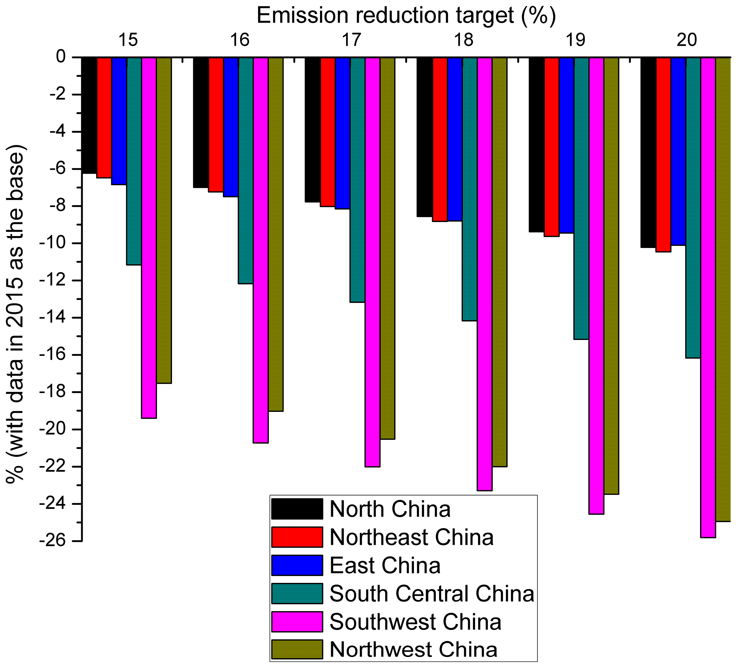
1. Carbon tax scenario in 2020

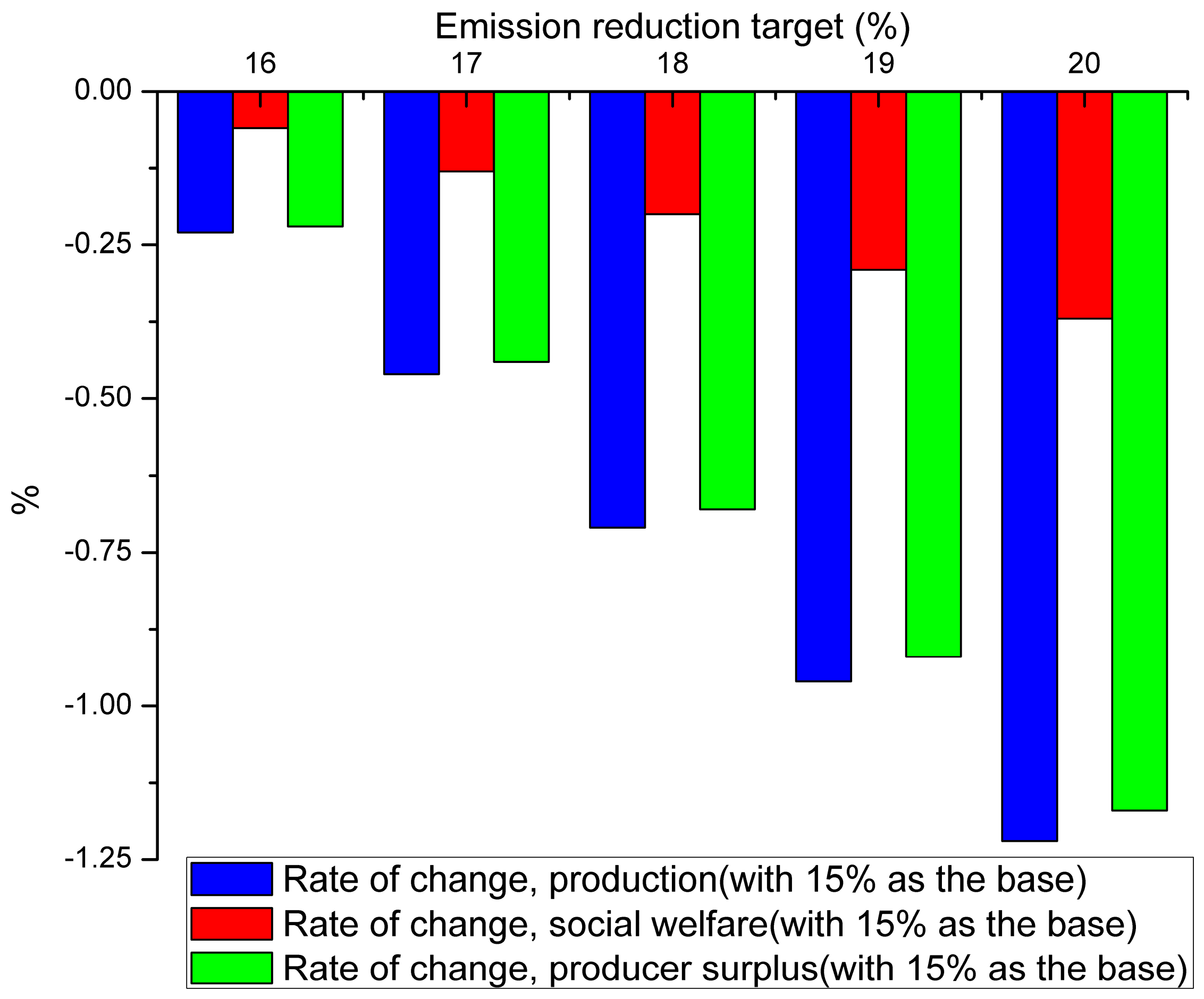
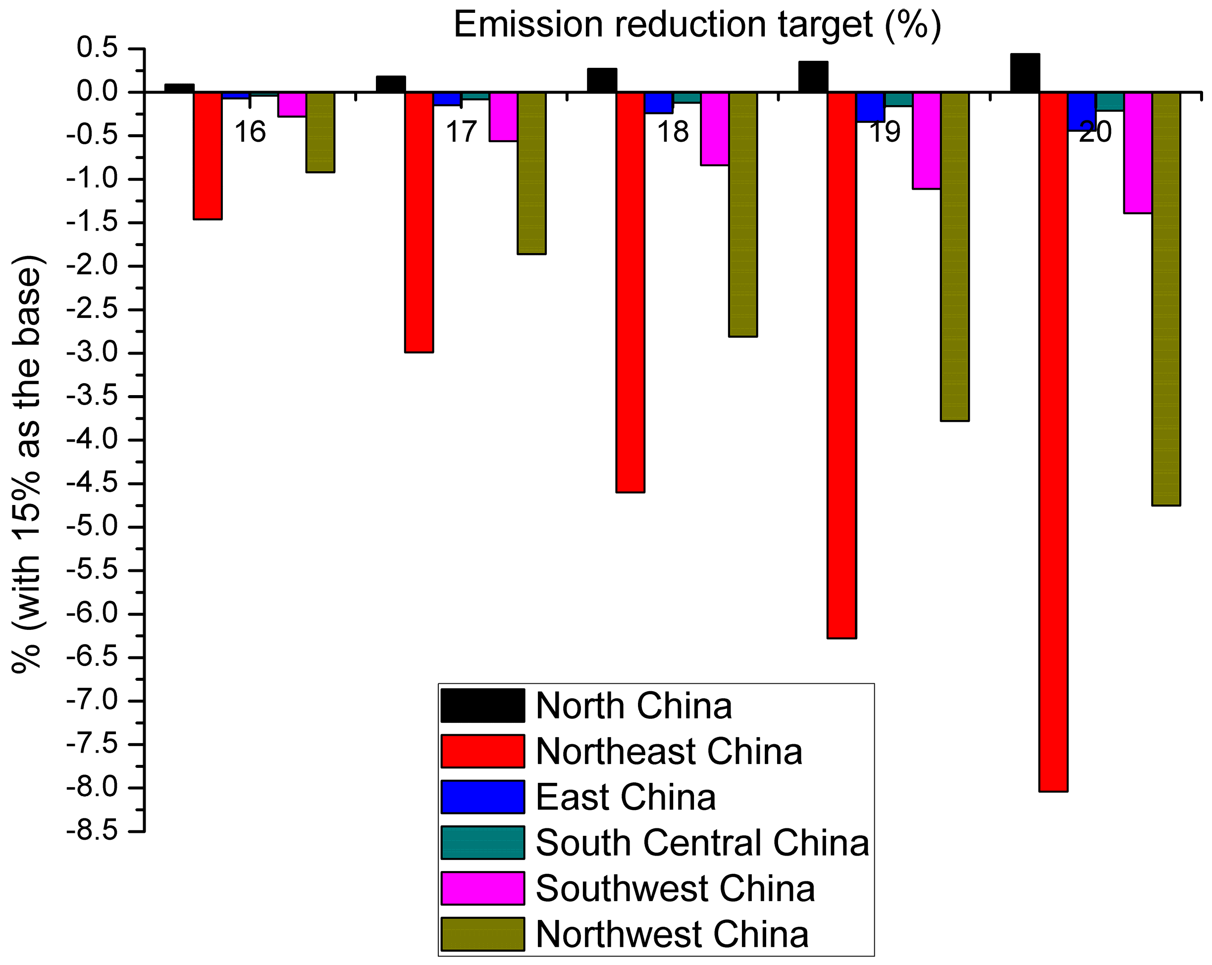
In this scenario, we assume that by 2020, the steel industry’s CO₂ intensity will fall by at least 15% compared to in 2010. Given that technological innovation alone will not be sufficient for high carbon-intensity reduction, the carbon tax will be a necessary policy tool. The solution for this scenario is similar to that of Case 1. Then, we calculate the corresponding results of social welfare and investigate scenarios in which the intensity of CO₂ emissions dropped from 15 to 20%.

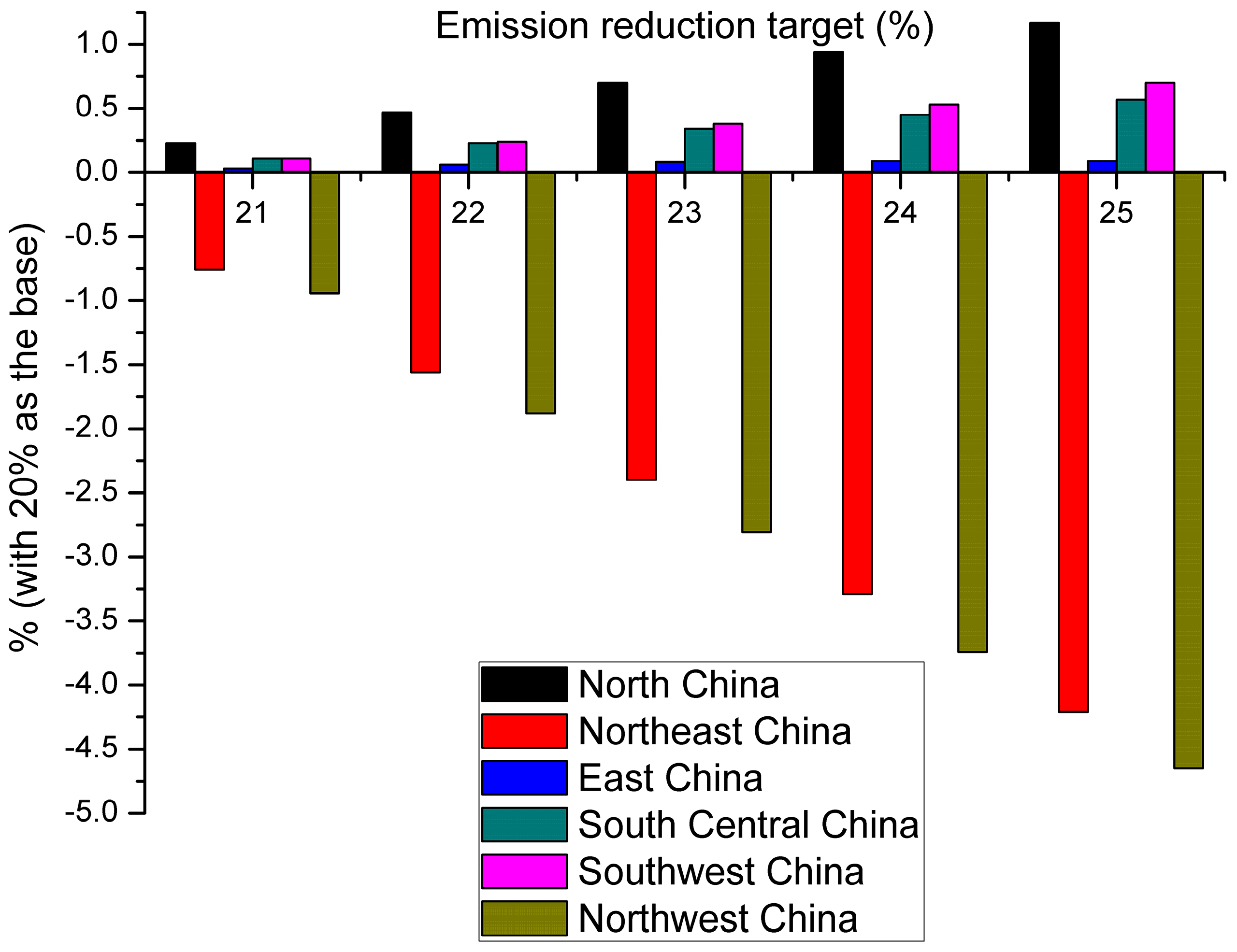
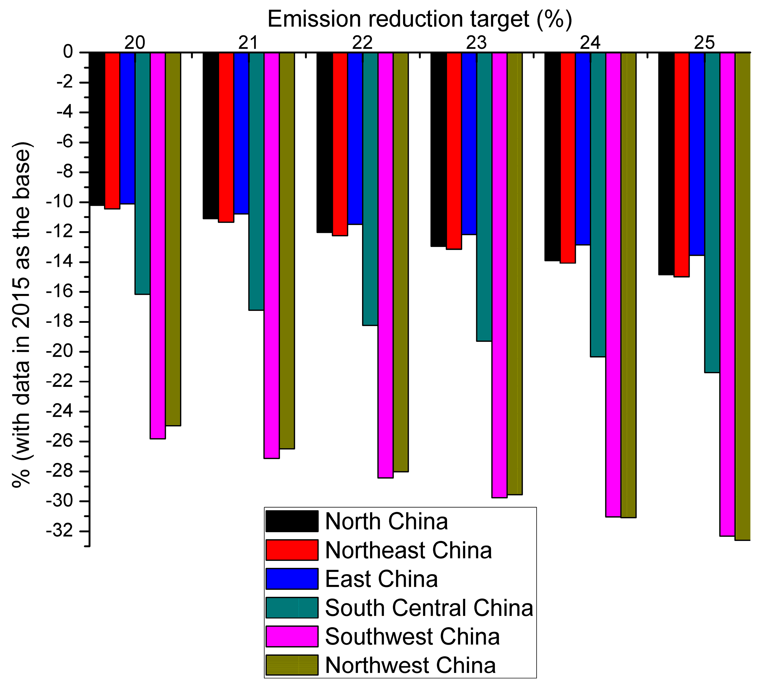
2. Carbon tax and product subsidy scenario in 2025

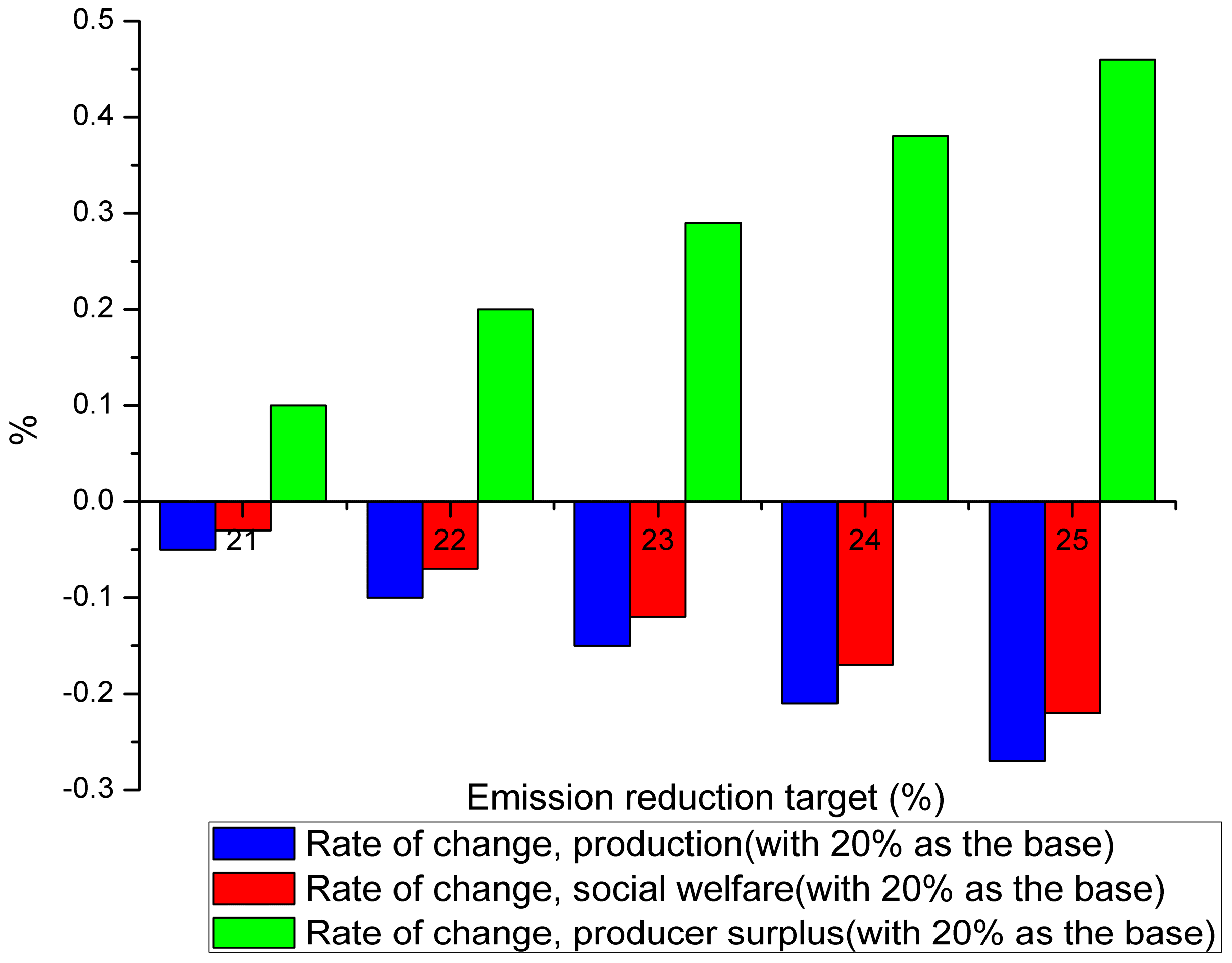
In this scenario, we assume that by 2025, the CO₂ intensity of the steel industry will fall by at least 20% compared to that in 2010. Again, because technological innovation alone will not be sufficient for high carbon-intensity reduction, the carbon tax will be a necessary policy tool. However the carbon tax levy has greatly increased the industry’s investment, and product subsides to producers can reduce the tax burden on producers while also meeting emissions demands. Thus, carbon tax and subsidy will comprise a dual method in 2025. The solution in this scenario corresponds to that of Case 2. Then, we calculate the social welfare results, and investigate scenarios in which the intensity of CO₂ emissions dropped by 20–25%.

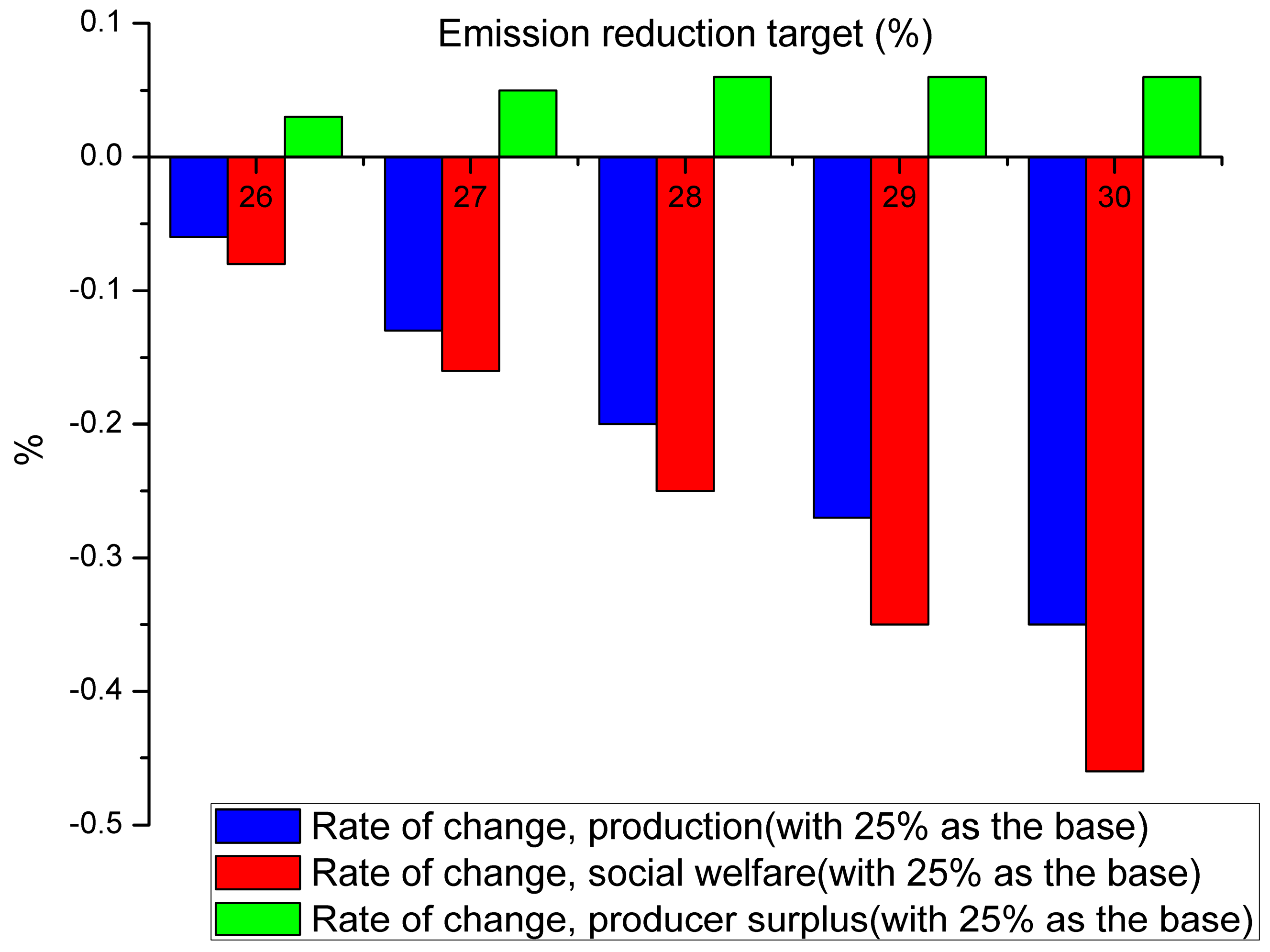
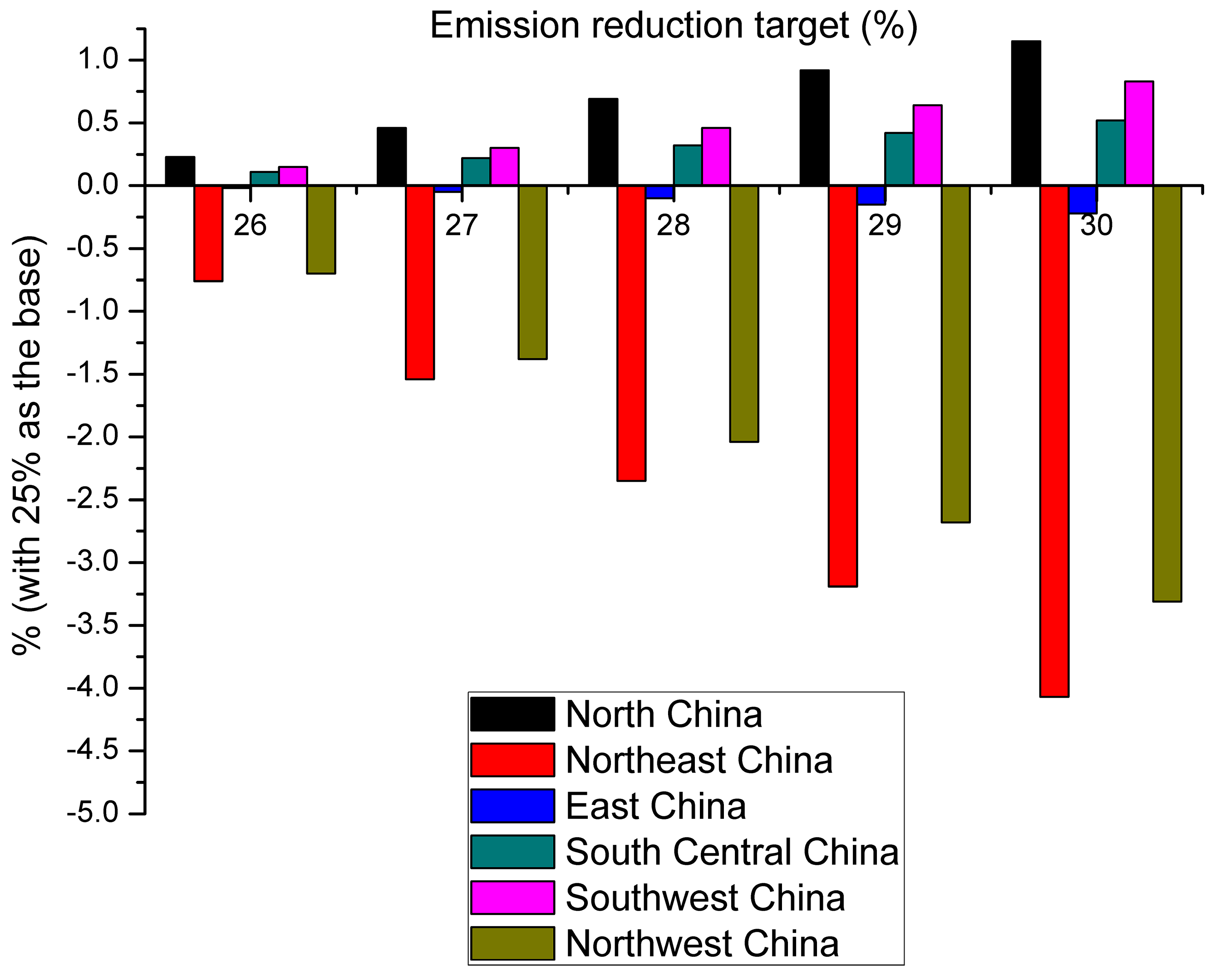
3. Carbon tax, product subsidy, and CCS demonstration project coexistence scenario in 2030

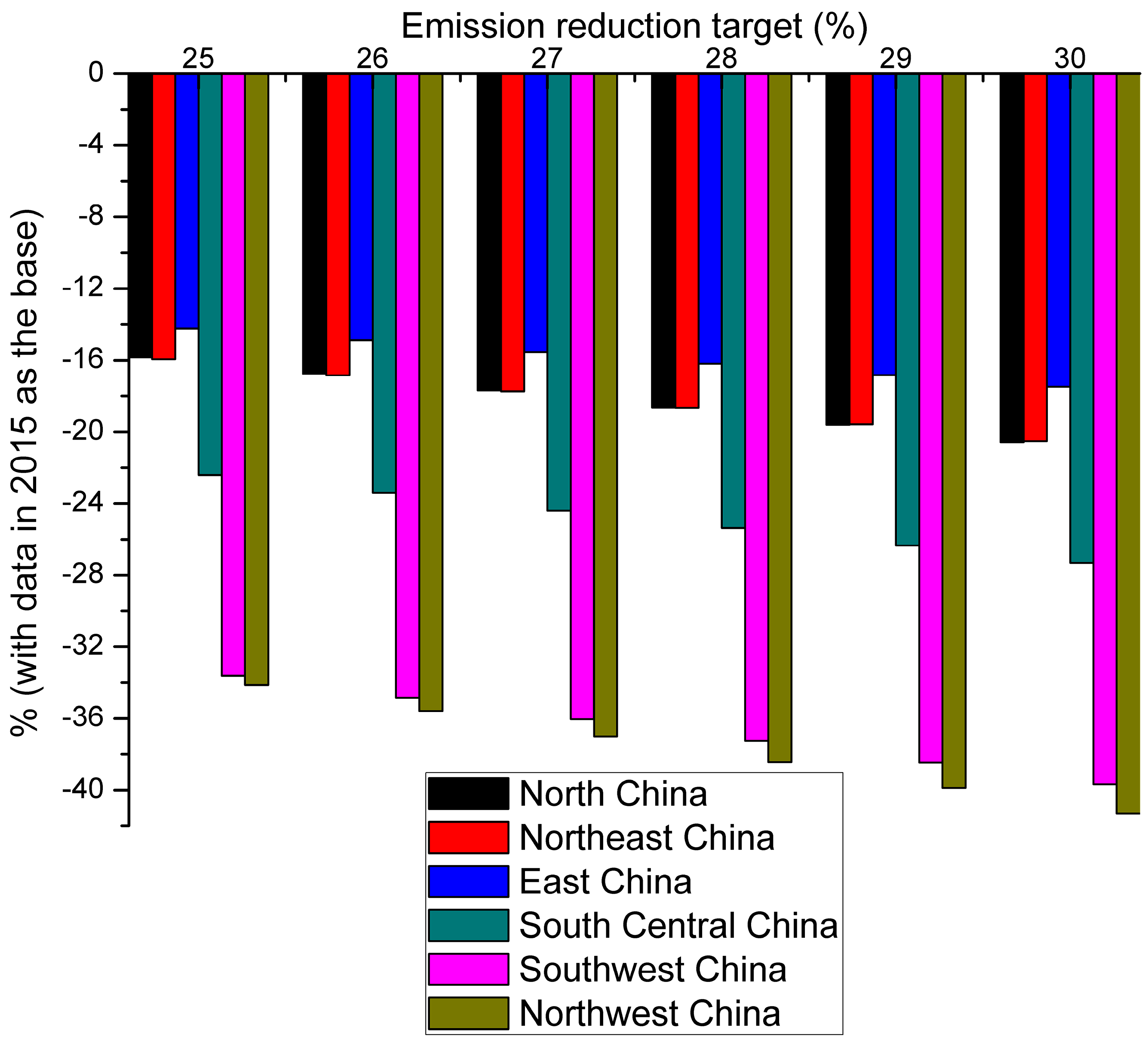
In contrast to 2010, we assume that the steel industry’s CO₂ intensity will fall by at least 25% by 2030. Again, because technological innovation alone will not be sufficient for high carbon-intensity reduction, the carbon tax and product subsidies will be necessary policy tools. With the improving CCS technology, large-scale CCS demonstration projects will be able to be applied to the steel industry. As a result, carbon tax, product subsidy, and CCS demonstration projects (i.e., 1–2 million ton CO₂ level) will be considered in 2030. The solution to this scenario corresponds to that of case 3. Then, we calculate the corresponding social welfare results, and investigate scenarios in which the intensity of CO₂ emissions dropped by 25–30%.

3.3. Parameters and Data Sources

In this paper, the CO₂ MAC (marginal abatement cost) results were derived from the CO₂ shadow price calculations in 2005–2015. According to [44,45,46], in the directional distance model the economic output is considered as desirable output, while CO₂ emissions is the undesirable output. An area’s production possibility is defined as: $P\left(x\right)=\left\{\left(y,b\right):xcanproduce\left(y,b\right)\right\}$. According to Färe’s [47] description of the directional distance function, we introduce the direction vector g = (g_y, g_b). The output-based distance function can be defined as follows:

$$D\left(x,y,b;g_y,g_b\right)=\max \{\beta :\left(y+\beta g_y,b-\beta g_b\right)\in P\left(x\right)\}$$

(10)

According to the method of nonparameter linear programming, the objective function is calculated as follows:

$$\begin{array}{l}{D}_k\left(x_k,y_k,b_k;g_y,g_b\right)=\max {\beta }_k\\ s.t.& {\displaystyle \sum _{j=1}^n{\lambda }_j{x}_j\le }{x}_k,\\ & {\displaystyle \sum _{j=1}^n{\lambda }_j{y}_j\ge y_k+{\beta }_k{g}_y},\\ & {\displaystyle \sum _{j=1}^n{\lambda }_j{b}_j=b_k-{\beta }_k{g}_b,}\\ & {\lambda }_j\ge 0,j=1,2,\dots n\end{array}$$

(11)

According to Lee [48], the undesirable output shadow price calculation formula can be written as:

$$q=p\times \frac{\partial D\left(x,y^{\ast },b^{\ast }\right)/\partial b^{\ast }}{\partial D\left(x,y^{\ast },b^{\ast }\right)/\partial y^{\ast }}\times \frac{{\sigma }_b}{{\sigma }_y}$$

(12)

Then, according to the six regions’ respective shadow price, the MACs of each region were fitted. The main parameters of each region are shown in

Table 2. The result of parameter fitting in formula.

Notations	Value	Unit
α	15,668.39	Yuan
β	$1.117\times {10}^{-5}$
e	2.79	t CO2/t
θ	14.55	Yuan/t CO2
m	$[1\times {10}^6,2\times {10}^6]$	t
A	204.96
B	$1.153\times {10}^7$	Yuan

.

The external macroscopic loss parameters of CO₂ emissions refer to Giorgio Guenno and Silvia Tiezzi [49], converted into 14.55 yuan per ton of CO₂.

In 2030, we assume that the steel industry will plan to build 1-2 million ton demonstration projects funded by the government. The cost curve refers to [50,51,52,53], and the linear curve is $M=204.96m+11.53\times {10}^6,m\in \left[1\times {10}^6,2\times {10}^6\right]\mathrm{ton}$. The unit is RMB.

Provincial steel production data, economic data, and employee data were collected from the China Statistical Yearbook [54,55,56,57,58,59,60,61,62,63,64,65], China’s Industrial Statistics Yearbook [66,67,68,69,70,71,72,73,74,75,76,77], and the China Steel Industry yearbook from 2005 to 2016 [78,79,80,81,82,83,84,85,86,87,88,89]. Energy consumption data came from the China Energy Statistics Yearbook [90,91,92,93,94,95,96,97,98,99,100,101] and each province’s Statistical Yearbook from 2005 to 2016. Economic data were calculated at the 2010 year price. In addition, CO₂ emissions in industrial production (IPPU CO₂) are included in this paper which also produce large amounts of CO₂. Therefore, CO₂ emissions accounting, emissions intensity and descent amplitude are based on energy consumption + IPPU CO₂ emissions.

Due to data availability, the steel industry’s relevant energy consumption and economic data were derived from the ferrous metal smelting and calendering processing industry in the Statistical Yearbook. The CO₂ accounting of fossil energy consumption and IPPU refer to IPCC2006 [102] and Duan et al. [103].

4. Results and Discussions

4.1. The Results of Parameter Fitting

The production cost takes into account the current trend of steel development in China, based on average production costs of 2010–2015. The descent amplitude of different regions is controlled at 5–30%. The parameter fitting conditions are shown in Table 2 and

Table 3. The result of parameter fitting in different regions.

Notations	Unit		i = 1	i = 2	i = 3	i = 4	i = 5	i = 6
e2015,i	t CO2/t		2.34	3.53	2.81	2.85	3.40	4.49
ai			954.57	886.60	2847.60	325.81	78.91	178.12
bi			702.15	567.70	9983.42	832.07	91.47	251.25
C0,i	Yuan	2020	3660.25	5469.57	3734.81	3910.43	5246.81	4759.35
		2025	3108.44	4646.29	2986.07	3326.32	4724.05	4520.52
		2030	2799.50	3944.25	2685.82	2997.62	4008.86	3844.57

.

4.2. Empirical Analysis

In the second stage of the game, the regional emissions and intensity of the steel industry are determined by its first-order conditions:

$$\begin{array}{l}\partial {\pi }_i/\partial q_i=0\\ \partial {\pi }_i/\partial r_i=0\end{array}$$

(13)

The relationship between steel production, the descending amplitude and t, η of each region is obtained by solving the simultaneous equations. The equilibrium yield and emissions reduction of the second stage in different situations can be determined by t, η.

Then we put the equilibrium output and emission reduction determined by t, η into the first stage to get the expression formula of social economic welfare (W). In the first stage of the game, the government maximizes the level of social economic welfare determined by t, η. Finally, we get W and other corresponding conclusions.

4.2.1. 2020 Scenario

In 2020, the carbon tax will be the only emissions reduction policy. With the gradual rise of in reduction targets, the carbon tax value and its total scale have increased gradually. In particular, the carbon tax value has risen rapidly from 65.88 yuan/t to 114.69 yuan/t, and the total carbon tax levy rose 61.84%.

Total output, overall social welfare function, consumer surplus, producer surplus and emissions loss have all shown a downward trend, the total output remained at around 0.835-0.846 million tons. Compared with 1.123 billion tons in 2015, output will have dropped by more than 20%, suggesting that in terms of satisfying social welfare functions, the demand for China’s steel industry market will also decrease significantly by 2020. This is in line with the current economic situation and the development of the steel industry. With the gradual rise in reduction targets, the total output, social welfare function, consumer surplus, producer surplus, and emissions losses are projected to fall by 1.22%, 0.37%, 2.43%, 1.17% and 7.03% respectively.

For the sub-regions, to reach the 15–20% target, the selection of emissions intensity and production yield are taken between regions. Emissions reduction efforts have increased in line with more ambitious reduction goals, but there are notable inter-regional differences. In the southwest and northwest regions, the intensity of emissions reduction is more than 20% in most cases. With an overall reduction target of 20%, the reduction in southwest China is the largest, at 25.81%. The reduction range is comparatively smaller in East China, North China and other places (approximately 6–10%) due to differences in production costs and emissions intensity. With the gradual increase in emissions reduction targets, except for in North China (0.44%), steel outputs in the rest regions of China are declining. The Northeast region has fallen especially significantly, by more than 8%. The results are shown in

Table 4. The result of overall iron and steel industry in 2020 scenario.

Emission Reduction Target	15%	16%	17%	18%	19%	20%
Carbon tax value (Yuan)	65.88	74.75	84.06	93.83	104.03	114.69
Production (100 million tons)	8.4584	8.4394	8.4194	8.3987	8.3773	8.3552
Rate of change, production (with 15% as the base)	-	−0.23%	−0.46%	−0.71%	−0.96%	−1.22%
Rate of change, social welfare (with 15% as the base)	-	−0.06%	−0.13%	−0.20%	−0.29%	−0.37%
Rate of change, producer surplus (with 15% as the base)	-	−0.22%	−0.44%	−0.68%	−0.92%	−1.17%

and

Table 5. The result of regions’ iron and steel industry in 2020 scenario.

Emission Reduction Target		15%	16%	17%	18%	19%	20%
Production (100 million tons)	North China	2.1579	2.1598	2.1617	2.1636	2.1655	2.1674
	Northeast China	0.4705	0.4636	0.4564	0.4488	0.4409	0.4327
	East China	2.0304	2.0289	2.0273	2.0255	2.0235	2.0213
	South Central China	1.9103	1.9096	1.9088	1.9080	1.9072	1.9063
	Southwest China	0.8197	0.8174	0.8151	0.8128	0.8106	0.8084
	Northwest China	1.0700	1.0602	1.0501	1.0399	1.0296	1.0192
Rate of change, production (with 15% as the base)	North China	-	0.09%	0.18%	0.27%	0.35%	0.44%
	Northeast China	-	−1.46%	−2.99%	−4.60%	−6.28%	−8.04%
	East China	-	−0.07%	−0.15%	−0.24%	−0.34%	−0.44%
	South Central China	-	−0.04%	−0.08%	−0.12%	−0.16%	−0.21%
	Southwest China	-	−0.28%	−0.56%	−0.84%	−1.11%	−1.39%
	Northwest China	-	−0.92%	−1.86%	−2.81%	−3.78%	−4.75%
The decline range of emission intensity (with data in 2015 as the base)	North China	6.23%	6.99%	7.77%	8.56%	9.38%	10.22%
	Northeast China	6.48%	7.24%	8.02%	8.82%	9.63%	10.46%
	East China	6.84%	7.49%	8.15%	8.80%	9.45%	10.11%
	South Central China	11.16%	12.17%	13.17%	14.17%	15.17%	16.17%
	Southwest China	19.41%	20.72%	22.01%	23.29%	24.55%	25.81%
	Northwest China	17.53%	19.03%	20.52%	22.00%	23.48%	24.95%

and Figure 1, Figure 2 and Figure 3.

4.2.2. 2025 Scenario

In 2025, emissions reduction policies should include carbon taxes and product subsidies. With the gradual increase in reduction targets, carbon tax and the total scale of carbon tax, unit subsidy value and total subsidies will increase as well. The carbon tax value will have risen from 114.64 yuan/t to 178.04 yuan/t, and the levy of the total carbon tax also rises 45.19%. The unit subsidy value will have risen from 289 yuan/t to 421 yuan/t, and the total subsidy rises 45.28%. However, the carbon tax is not fully subsidized to steel companies, a very small surplus remains.

Total production will remain at around 900 million tons, although the pressure to reduce emissions will continue to rise to a 20–25% range compared with a modest increase in output in 2020. In this scenario, and with the gradual rise in reduction targets, total output, total social welfare, consumer surplus, producer surplus, and emissions losses should fall by 0.27%, 0.22%, 0.54%, 0.46%, and 6.51% respectively, and a slower rate of decline in 2020. Even when the target of reducing emissions increases, the producer surplus does the same, this suggests that although the target is more ambitious, CO₂ emissions tax subsidies for the enterprise can increase producers’ enthusiasm for production, and help to increase total output and other corresponding indicators.

For the sub-region to reach the 20–25% target, emissions intensity and production yield are taken between regions. Emissions reduction efforts have increased in line with more ambitious reduction goals, but there are again notable inter-regional differences. In Southwest and Northwest China, the intensity of emissions reduction will have exceeded 25% in most cases. With an overall drop target of 25%, the reduction in Northwest China is the largest, at 32.6%. Relatively speaking, the reduction is smaller in East China, North China and other places, only 10–15%. It is slightly higher in South Central China, at 16–21%. In terms of output, the difference in production costs and the intensity of emissions reduction, combined with carbon tax and return subsidies, render significant changes in yield. The output in North China, East China, South Central China and Southwest China show a rising trend, whereas declines Northeast and Northwest China by approximately 4%. The results are shown in

Table 6. The result of overall iron and steel industry in 2025 scenario.

Emission Reduction Target	20%	21%	22%	23%	24%	25%
Carbon tax value (Yuan)	114.64	126.34	138.52	151.18	164.43	178.04
Unit value of subsidy (Yuan)	289.00	314.50	340.50	367.00	394.00	421.00
Production (100 million tons)	9.0203	9.0160	9.0114	9.0065	9.0013	8.9985
Rate of change, production (with 20% as the base)	-	−0.05%	−0.10%	−0.15%	−0.21%	−0.27%
Rate of change, social welfare (with 20% as the base)	-	−0.03%	−0.07%	−0.12%	−0.17%	−0.22%
Rate of change, producer surplus (with 20% as the base)	-	0.10%	0.20%	0.29%	0.38%	0.46%

and

Table 7. The result of regions’ iron and steel industry in 2025 scenario.

Emission Reduction Target		20%	21%	22%	23%	24%	25%
Production (100 million tons)	North China	2.2551	2.2603	2.2656	2.2709	2.2763	2.2816
	Northeast China	0.7635	0.7577	0.7516	0.7452	0.7384	0.7313
	East China	2.2818	2.2825	2.2831	2.2836	2.2838	2.2838
	South Central China	2.0230	2.0253	2.0276	2.0299	2.0322	2.0344
	Southwest China	0.8701	0.8711	0.8722	0.8734	0.8747	0.8762
	Northwest China	0.8268	0.8191	0.8113	0.8036	0.7959	0.7884
Rate of change, production (with 20% as the base)	North China	-	0.23%	0.47%	0.70%	0.94%	1.17%
	Northeast China	-	−0.76%	−1.56%	−2.40%	−3.29%	−4.21%
	East China	-	0.03%	0.06%	0.08%	0.09%	0.09%
	South Central China	-	0.11%	0.23%	0.34%	0.45%	0.57%
	Southwest China	-	0.11%	0.24%	0.38%	0.53%	0.70%
	Northwest China	-	−0.94%	−1.88%	−2.81%	−3.74%	−4.65%
The decline range of emission intensity (with data in 2015 as the base)	North China	0.1021	0.1111	0.1202	0.1295	0.1390	0.1485
	Northeast China	0.1046	0.1134	0.1224	0.1314	0.1407	0.1499
	East China	0.1010	0.1079	0.1148	0.1216	0.1285	0.1354
	South Central China	0.1616	0.1721	0.1825	0.1929	0.2034	0.2138
	Southwest China	0.2581	0.2713	0.2843	0.2974	0.3104	0.3232
	Northwest China	0.2494	0.2649	0.2802	0.2955	0.3109	0.3260

and Figure 4, Figure 5 and Figure 6.

4.2.3. 2030 Scenario

In 2030, emissions reduction policies should include carbon taxes, product subsidies, and CCS demonstration projects. With the gradual increase in reduction targets, come increases in the carbon tax and its total scale, unit subsidy value and total subsidies. The carbon tax value is projected to rise from 192.29 yuan/t to 266.17 yuan/t, and the total carbon tax should increase 28.79%. The unit subsidy value will have risen from 455 yuan/t to 588 yuan/t, and the total subsidy rose 28.78%. However, the carbon tax is not fully subsidized to steel companies, there is still a very small surplus. The CO₂ emissions from the CCS demonstration project also show an increase, with the target of 30% (M = 1.9 million tons) and a 44.24% increase in funding for CCS projects.

Total production should remain at around 935 million-938 million tons, although the pressure continues to increase to 25–30%, compared with a modest increase in production in 2020. In this scenario, with the gradual increase of reduction targets, total output, social welfare function, consumer surplus, producer surplus, and emissions losses are projected to fall by 0.35%, 0.46%, 0.69%, 0.06%, and 6.96% respectively, which also occurs alongside an increasing emissions reduction target. The producer surplus will increase as well. This shows that although the target is more ambitious, CO₂ emissions tax subsidies to enterprises and CCS can increase producers’ enthusiasm for production, and help to increase total output and other corresponding indicators.

In order for sub-regions to reach the 25–30% target, emission intensity and production yield are taken between regions. Emissions reduction efforts have increased in line with more ambitious reduction goals, but there are again notable inter-regional differences. In Southwest and Northwest China, the intensity of emission reduction exceeds 33% in most cases. With an overall drop target of 30%, the reduction in the Northwest region is the largest, at 41.31%. By comparison, the emissions reduction in East China is the smallest (14–17%). The drop range in Northeast China, North China and other places is only 15–20%. It is slightly higher in South Central China at 22–27%. In terms of output, the difference in production costs and the intensity emissions reduction, combined with the carbon tax and return subsidies, affect yield changes. The output in North China, South Central China and Southwest China show a rising trend, whereas it is declining in Northeast, East and Northwest China. The Northeast region is projected to fall by more than 4%. The results are shown in

Table 8. The result of overall iron and steel industry in 2030 scenario.

Emission Reduction Target	25%	26%	27%	28%	29%	30%
Carbon tax value (Yuan)	192.29	206.24	220.58	235.27	250.39	266.17
Unit value of subsidy (Yuan)	455.00	481.50	508.00	534.50	561.00	588.00
The CO2 emission reduced by CCS demonstration project (million tons)	1.30	1.30	1.40	1.70	2.00	1.90
Production (100 million tons)	9.3831	9.3773	9.3710	9.3646	9.3577	9.3505
Rate of change, production (with 25% as the base)	-	−0.06%	−0.13%	−0.20%	−0.27%	−0.35%
Rate of change, social welfare (with 25% as the base)	-	−0.08%	−0.16%	−0.25%	−0.35%	−0.46%
Rate of change, producer surplus (with 25% as the base)	-	0.03%	0.05%	0.06%	0.06%	0.06%

and

Table 9. The result of regions’ iron and steel industry in 2030 scenario.

Emission Reduction Target		25%	26%	27%	28%	29%	30%
Production (100 million tons)	North China	2.1759	2.1810	2.1860	2.1910	2.1959	2.2009
	Northeast China	0.9648	0.9574	0.9499	0.9420	0.9339	0.9254
	East China	2.1704	2.1699	2.1692	2.1683	2.1671	2.1656
	South Central China	1.9433	1.9455	1.9476	1.9496	1.9516	1.9525
	Southwest China	1.1304	1.1320	1.1338	1.1356	1.1376	1.1397
	Northwest China	0.9984	0.9914	0.9846	0.9780	0.9716	0.9654
Rate of change, production (with 25% as the base)	North China	-	0.23%	0.46%	0.69%	0.92%	1.15%
	Northeast China	-	−0.76%	−1.54%	−2.35%	−3.19%	−4.07%
	East China	-	−0.02%	−0.05%	−0.10%	−0.15%	−0.22%
	South Central China	-	0.11%	0.22%	0.32%	0.42%	0.52%
	Southwest China	-	0.15%	0.30%	0.46%	0.64%	0.83%
	Northwest China	-	−0.70%	−1.38%	−2.04%	−2.68%	−3.31%
The decline range of emission intensity (with data in 2015 as the base)	North China	0.1583	0.1676	0.1770	0.1865	0.1960	0.2058
	Northeast China	0.1594	0.1684	0.1775	0.1866	0.1957	0.2051
	East China	0.1423	0.1488	0.1554	0.1618	0.1683	0.1749
	South Central China	0.2242	0.2341	0.2439	0.2536	0.2634	0.2732
	Southwest China	0.3362	0.3484	0.3605	0.3726	0.3846	0.3967
	Northwest China	0.3413	0.3558	0.3702	0.3844	0.3987	0.4131

and Figure 7, Figure 8 and Figure 9.

4.3. Discussion of Results

Current research on the future iron and steel industry emissions reduction targets is scarce, therefore, this paper does not discuss optimal emissions intensity. Only the aforementioned three scenarios were analyzed. Moreover, because of certain assumptions in the model, there were some gaps between the calculations and the actual results, but some trends and rules can still be found and identified.

On a national scale, with the gradual increase in reduction targets, the overall social welfare, consumer surplus, output and emission losses appear to be decreasing. The trend of carbon tax value, total carbon tax, unit value of output subsidies and total subsidies are rising. The change in producer surplus is irregular due to the comprehensive influence of production cost, production yield, carbon tax and subsidies.

Judging by the change range of the results, if only one emission reduction policy is considered, the overall social welfare, consumer surplus, output and loss are sharper than the results of multiple reduction policies. The adoption of a variety of reduction policies can compensate for the weakness associated with a single reduction in production costs, slow down the increase range in production costs, so as to reduce the overall range of changes. The total carbon tax and subsides are closely related to the unit value of carbon tax and the value of subsidy. Given the gradual increase in reduction targets, the change of total carbon tax and total subsidy range are significant.

For sub-region, which differ in production costs and emissions reduction costs, the optimal emissions range and output choices are related to the carbon tax value and subsides in different scenarios. Therefore, the result of each situation are quite different. According to the relevant national policy [1]: North and East China should focus on the mitigation of regional environmental pressure, relying on dominant enterprises. Through the reduction of restructuring, significantly reduce the excess steel capacity significantly and achieve regional reduction targets. The Midwest and Northeast old industrial base should rely on enterprises’ regional comparative advantage, implement regional integration, and reduce the number of entrepreneurs and excess steel production capacity. Steel output is be expected to peak in 2015–2020 intervals.

Our calculations show that, in three cases, output reduces by 150 to 200 million tons compared to that in 2015, with total output of about 900 million tons. After implementing of different carbon emissions reduction policies, production in North and East China should decrease about 1/3, South Central China production should remain in 180–200 million tons. The Northeast, Southwest, and Northwest region will increase but a much smaller rate compared to the reduction in North and East China. Although East and North China are still the main steel producing areas (about 50%), the output transition between the regions is from polarization to average. The polarization phenomenon appears to be easing, the regional maximum production ratio has declined from 10:1 to about 3:1. The results show a certain reference value in this calculation. Judging from the policy analysis aimed at “resolving excess capacity, prohibiting new capacity, production and consumption will enter the peak to the downward period” [1], the model and results have a certain reference value.

5. Conclusions

In light of the medium-and long-range plan promulgated by the government, a two-stage dynamic game model was constructed which incorporated the carbon tax, product subsidy, CCS, and other factors into the system of emission reduction mechanism. Then, we examined the resultant effects and economic impacts on six regions and China’s overall steel industry. The model is the abstraction and assumption of a practical problem, so the calculation results may exist a little deviate from the actual situation, which makes the research result have some deviations. This paper emphasizes the change trends of corresponding indicators with increasing governmental pressure to reduce emissions. The main conclusions are as follows:

(I)

Under a certain emissions reduction policy, with the gradual increase in reduction targets, the overall social welfare, consumer surplus, output and emissions losses are trending downward. The carbon tax unit value, total carbon tax, output subsidy unit value, and total subsidies demonstrate a rising trend.

(II)

With the increasing target of reducing emissions, a variety of emissions reduction policies are more effective than a single reduction policy, which can slow down the indicators’ decreasing range.

(III)

For enterprises in the sub-regions, each region needs to choose its own reduction range and output. With the gradual increase in reduction targets, regional output has not shown a complete downward trend. Regional output has instead increased in some places likely duo to production function, carbon tax, subsidy and other comprehensive factors.

(IV)

In the future, East and North China are expected to remain the primary producing areas, however, the proportion of production in the Northeast, Southwest and Northwest regions could rise. With the implementation of various emissions reduction policies, regional output polarization has eased.

Based on the above results and conclusions, when formulating emissions reduction targets and ancillary emissions reduction policies, the Chinese steel industry should use technological advances (i.e., lower production costs) along with several reasonable emissions reduction measures to achieve reduction targets into consideration. CCS can be implemented when the targets are too extreme and the CCS technology reaches a certain level. In future research, the impact of emissions reduction measures on the Chinese steel industry economy will be considered in the context of large-scale investment in CCS projects.

Secondly, China’s steel industry is currently at overcapacity, that is, production capacity is far greater than the actual consumption. This paper’s calculations show that when the market equilibrium is reached, the output and consumption of steel will be lower than they are at present.

Therefore, to alleviate the overcapacity contradiction and bring relief to the entire industry, China’s steel industry needs to ban new steel production and push obsolete companies and backward-producing enterprises out of the market as soon as possible. In the future, the government could levy more emission tax, reduce subsidies and conduct related policy research to address backward capacity, high-pollution emissions enterprises. These methods and impacts will be considered in subsequent research.

Thirdly, to improve the steel layout, the government should consider market demand, transportation, environment capacity and energy resources support conditions overall. Combined with solutions to address excess capacity and deepen regional layout reduction adjustments, the government should also encourage large-scale enterprises to reduce production capacity initiatively. Coastal areas’ government should change their ideas. The blind relocation of steel enterprises from inland to coastal areas should be banned. And no longer layout the new coastal base. Based on the existing coastal base, the government should implement the “group development” to improve the quality and efficiency. Inland regions should take the regional market capacity and energy resources to support as the double bottom line, and withdraw non-competitive enterprises resolutely. Based on existing leading enterprises, the regional government should aim to integrate relief development, achieve a balance between regional steel productions and reduce polarization.

References

1. Ministry of Industry and Information Technology of the People’s Republic of China. Available online: http://www.miit.gov.cn/n1146285/n1146352/n3054355/n3057569/n3057573/c5353862/content.html (accessed on 14 November 2016).
2. Jorgenson, D.W.; Peter, J.W. Intertemporal General Equilibrium Modeling of U.S. Environmental Regulation. J. Policy Model. 1990, 12, 715–744. [Google Scholar] [CrossRef]
3. Jorgenson, D.W.; Peter, J.W. Reducing U.S. Carbon Dioxide Emissions: The Cost of Different Goals. Adv. Econ. Energy Resour. 1992, 7, 125–158. [Google Scholar]
4. Manne, A.S.; Mendelsohn, R.; Richels, R. MERGE: A model for evaluating regional and global effects of GHG reduction policies. Energy Policy 1995, 23, 17–34. [Google Scholar] [CrossRef]
5. Jorgenson, D.W.; Peter, J.W. Fundamental U.S. Tax Reform and Energy Markets. Energy J. 1997, 18, 1–30. [Google Scholar] [CrossRef]
6. Zhang, Z.X. Macroeconomic Effects of CO2 Emission Limits: A Computable General Equilibrium Analysis for China. J. Policy Model. 1998, 20, 213–250. [Google Scholar] [CrossRef]
7. Fan, Z.; Li, S.T. Structural Change and Pollution Emission-perspective and policy impact analysis. J. Quant. Tech. Econ. 1998, 8, 8–14. [Google Scholar]
8. Jian, X.; Saltzman, S. Environmental Policy Analysis: An Environmental Computable General-Equilibrium Approach for Developing Countries. J. Policy Model. 2000, 22, 453–489. [Google Scholar]
9. Jian, X. An Environmentally Extended Social Accounting Matrix. Environ. Resour. Econ. 2000, 16, 391–406. [Google Scholar]
10. Kemfert, C.; Welsch, H. Energy capital labor Substitution and the economic effects of CO2 abatement: Evidence for Germany. J. Policy Model. 2000, 22, 641–660. [Google Scholar] [CrossRef]
11. Wendner, R. An Applied Dynamic General Equilibrium Model of Environmental Tax Reforms and Pension Policy. J. Policy Model. 2001, 23, 25–50. [Google Scholar] [CrossRef]
12. Van Heeden, J.; Gerlagh, R.; Blignaut, J.; Horridge, M.; Hess, S.; Mabugu, R.; Mabugu, M. Searching for triple dividends in South Africa: Fighting CO2 pollution and poverty while promoting growth. Energy J. 2006, 27, 113–141. [Google Scholar] [CrossRef]
13. Abrell, J. Regulating CO2 emissions of transportation in Europe: A CGE analysis using market-based instruments. Transp. Res. Part D 2010, 15, 235–239. [Google Scholar] [CrossRef]
14. Benavides, C.; Gonzales, L.; Diaz, M.; Fuentes, R.; García, G.; Palma-Behnke, R.; Ravizza, C. The Impact of a Carbon Tax on the Chilean Electricity Generation Sector. Energies 2015, 8, 2674–2700. [Google Scholar] [CrossRef]
15. Yahoo, M.; Othman, J. Employing a CGE model in analysing the environmental and economy-wide impacts of CO2 emission abatement policies in Malaysia. Sci. Total Environ. 2017, 584–585, 234–243. [Google Scholar] [CrossRef] [PubMed]
16. Liang, Q.M.; Fan, Y.; Wei, Y.M. Carbon taxation policy in China: How to protect energy and trade intensive sectors? J. Policy Model. 2007, 29, 311–333. [Google Scholar] [CrossRef]
17. Yang, L.; Mao, X.Q.; Liu, Q.; Liu, Z.Y. Impact Assessment for Energy Taxation Policy Based on A Computable General Equilibrium (CGE) Model. China Popul. Resour. Environ. 2009, 19, 24–29. [Google Scholar]
18. Wu, L.B.; Qian, H.Q.; Tang, W.Q. Selection Mechanism between Emission Trading and Carbon Tax based on Simulation of Dynamic Marginal Abatement Cost. Econ. Res. J. 2014, 9, 48–61. [Google Scholar]
19. Xu, S.C.; Zhang, W.W. Analysis of impacts of carbon taxes on China’s economy and emissions reduction under different refunds: Based on dynamic CGE Model. China Popul. Resour. Environ. 2016, 26, 46–54. [Google Scholar]
20. Chen, W.; Zhou, J.F.; Li, S.Y.; Li, Y.C. Effects of an Energy Tax (Carbon Tax) on Energy Saving and Emission Reduction in Guangdong Province-Based on a CGE Model. Sustainability 2017, 9. [Google Scholar] [CrossRef]
21. Ling, T.; Shi, J.R.; Yu, L.; Qin, B. Economic and environmental influences of coal resource tax in China: A dynamic computable general equilibrium approach. Resour. Conserv. Recycl. 2017, 117, 34–44. [Google Scholar]
22. Montero, J.P. Permits, Standards, and Technology Innovation. J. Environ. Econ. Manag. 2002, 44, 23–44. [Google Scholar] [CrossRef]
23. Bruneau, J.F. A Note on Permits, Standards, and Technology Innovation. J. Environ. Econ. Manag. 2004, 48, 1192–1199. [Google Scholar] [CrossRef]
24. Requate, T. Dynamic incentives by environmental policy instruments—A survey. Ecol. Econ. 2005, 54, 175–195. [Google Scholar] [CrossRef]
25. Requate, T. Timing and commitment of environmental policy, adoption of new technology, and repercussions on R & D. Environ. Resour. Econ. 2005, 31, 175–199. [Google Scholar]
26. Puller, S. The strategic use of innovation to influence regulatory standard. J. Environ. Econ. Manag. 2006, 52, 690–706. [Google Scholar] [CrossRef]
27. Poyago-Theotoky, J.; Teerasuwannajak, K. The Timing of Environmental Policy: A Note on the Role of Product Differentiation. J. Regul. Econ. 2002, 21, 305–316. [Google Scholar] [CrossRef]
28. Poyago-Theotoky, J.A. The organization of R & D and environmental policy. J. Econ. Behav. Organ. 2007, 62, 63–75. [Google Scholar]
29. Youssef, S.B.; Zaccour, G. Absorptive Capacity, R & D Spillovers, Emissions Taxes and R & D Subsidies. Strateg. Behav. Environ. 2014, 4, 41–58. [Google Scholar]
30. Ouchida, Y.; Goto, D. Cournot Duopoly and Environmental R & D under Regulator’s Precommitment to an Emissions tax. Appl. Econ. Lett. 2016, 23, 324–331. [Google Scholar]
31. Moner-Colonques, R.; Rubio, S.J. The Strategic Use of Innovation to Influence Environmental Policy: Taxes versus Standards. B.E. J. Econ. Anal. Policy 2016, 16, 973–1000. [Google Scholar] [CrossRef]
32. Demailly, D.; Quirion, P. European Emission Trading Scheme and competitiveness: A case study on the iron and steel industry. Energy Econ. 2008, 30, 2009–2027. [Google Scholar] [CrossRef]
33. Cato, S. Environmental policy in a mixed market: Abatement subsidies and emissions taxes. Environ. Econ. Policy Stud. 2011, 13, 283–301. [Google Scholar] [CrossRef]
34. Eyland, T.; Zaccour, G. Strategic Effects of a Border Tax Adjustment. Int. Game Theory Rev. 2012, 14, 31–42. [Google Scholar] [CrossRef]
35. Ouchida, Y.; Goto, D. Do emission subsidies reduce emission? In the context of environmental R & D organization. Econ. Model. 2014, 36, 511–516. [Google Scholar]
36. McDonald, S.; Poyago-Theotoky, J. Green technology and optimal emissions taxation. J. Public Econ. Theory 2017, 19, 362–376. [Google Scholar] [CrossRef]
37. Lambertini, L.; Poyago-Theotoky, J.; Tampieri, A. Cournot Competition and “Green” Innovation: An Inverted-U Relationship. Energy Econ. 2017, 68, 116–123. [Google Scholar] [CrossRef]
38. Li, C.S.; Fan, Y.; Zhu, L. Emissions Tax and Its Revenue Refunding Scheme Design with Exogenous Abatement Target. Syst. Eng. 2012, 30, 82–86. [Google Scholar]
39. Li, C.S.; Fan, Y.; Zhu, L. The study of Carbon Dioxide Emission Intensity Abatement Mechanism of Iron and Steel Industry Based on Two-Stage Game Model. Chin. J. Manag. Sci. 2012, 20, 93–100. [Google Scholar] [CrossRef]
40. Yu, W.S.; Zhang, Z.Y. Feasibility and Mode Selection of Carbon Tax Policy in China based on Game Theory. China Popul. Resour. Environ. 2013, 23, 8–15. [Google Scholar]
41. Li, Y.; Zhao, D.Z.; Zhu, X.G. A Game Model for Government and Enterprise Behavior Based on a Carbon Tax. Resour. Sci. 2013, 35, 125–131. [Google Scholar]
42. Qiao, H.; Song, N.; Gao, H.W. Analysis on the strategies of European Union’s airline carbon tax with Stackelberg game models. Syst. Eng. Theory Pract. 2014, 34, 158–167. [Google Scholar]
43. Xu, X.Y.; Xu, X.P.; He, P. Joint production and pricing decisions for multiple products with cap-and-trade and carbon tax regulations. J. Clean. Prod. 2016, 112, 4093–4106. [Google Scholar] [CrossRef]
44. Chen, S.Y. Industrial carbon dioxide shadow price: Parametric and nonparametric methods. World Econ. 2010, 8, 93–111. [Google Scholar]
45. Zhou, X.; Fan, L.W.; Zhou, P. Marginal CO2 abatement costs: Findings from alternative shadow price estimates for Shanghai industrial sectors. Energy Policy 2015, 77, 109–117. [Google Scholar] [CrossRef]
46. Chen, D.H.; Pan, Y.C.; Wu, C.Y. Marginal abatement costs of CO2 emission in China and its regional differences. China Popul. Resour. Environ. 2016, 10, 86–93. [Google Scholar]
47. Färe, R.; Grosskopf, S.; Pasurka, C.A., Jr. Environmental Production Functions and Environmental Directional Distance Functions. Energy 2007, 32, 1055–1066. [Google Scholar] [CrossRef]
48. Lee, J.D.; Park, J.B.; Kim, T.Y. Estimation of the shadow prices of pollutants with production/environment inefficiency taken into account: A nonparametric directional distance function approach. J. Environ. Manag. 2002, 64, 365–375. [Google Scholar] [CrossRef]
49. Guenno, G.; Tiezzi, S. The Index of Sustainable Economics Welfare (ISEW) for Italy; Nota Di Lavoro; Fondazione Eni Enrico Mattei: Milano, Italy, 1998. [Google Scholar]
50. Dahowski, R.T.; Li, X.; Davidson, C.L.; Wei, N.; Dooley, J.J.; Gentile, R.H. A Preliminary Cost Curve Assessment of Carbon Dioxide Capture and Storage Potential in China. Energy Procedia 2009, 1, 2849–2856. [Google Scholar] [CrossRef]
51. Liu, H.W.; Kelly, S.G. Preparing to ramp up large-scale CCS demonstrations: An engineering economic assessment of CO2 pipeline transportation in China. Int. J. Greenh. Gas Control 2011, 5, 798–804. [Google Scholar] [CrossRef]
52. Wang, B.Q.; Li, H.Q.; Bao, W.J. A model of economy for overall process of CO2 capture and saline storage. CIESC J. 2012, 63, 894–903. [Google Scholar]
53. Zhu, L.; Fan, Y. Modeling the Investment of Coal-fired Power Plant Retrofit with CCS and Subsidy Policy Assessment. China Popul. Resour. Environ. 2014, 24, 99–105. [Google Scholar]
54. National Bureau of Statistics of the People’s Republic of China. CSY, 2005. China Statistical Yearbook; National Bureau of Statistics of the People’s Republic of China: Beijing, China, 2005. [Google Scholar]
55. National Bureau of Statistics of the People’s Republic of China. CSY, 2006. China Statistical Yearbook; National Bureau of Statistics of the People’s Republic of China: Beijing, China, 2006. [Google Scholar]
56. National Bureau of Statistics of the People’s Republic of China. CSY, 2007. China Statistical Yearbook; National Bureau of Statistics of the People’s Republic of China: Beijing, China, 2007. [Google Scholar]
57. National Bureau of Statistics of the People’s Republic of China. CSY, 2008. China Statistical Yearbook; National Bureau of Statistics of the People’s Republic of China: Beijing, China, 2008. [Google Scholar]
58. National Bureau of Statistics of the People’s Republic of China. CSY, 2009. China Statistical Yearbook; National Bureau of Statistics of the People’s Republic of China: Beijing, China, 2009. [Google Scholar]
59. National Bureau of Statistics of the People’s Republic of China. CSY, 2010. China Statistical Yearbook; National Bureau of Statistics of the People’s Republic of China: Beijing, China, 2010. [Google Scholar]
60. National Bureau of Statistics of the People’s Republic of China. CSY, 2011. China Statistical Yearbook; National Bureau of Statistics of the People’s Republic of China: Beijing, China, 2011. [Google Scholar]
61. National Bureau of Statistics of the People’s Republic of China. CSY, 2012. China Statistical Yearbook; National Bureau of Statistics of the People’s Republic of China: Beijing, China, 2012. [Google Scholar]
62. National Bureau of Statistics of the People’s Republic of China. CSY, 2013. China Statistical Yearbook; National Bureau of Statistics of the People’s Republic of China: Beijing, China, 2013. [Google Scholar]
63. National Bureau of Statistics of the People’s Republic of China. CSY, 2014. China Statistical Yearbook; National Bureau of Statistics of the People’s Republic of China: Beijing, China, 2014. [Google Scholar]
64. National Bureau of Statistics of the People’s Republic of China. CSY, 2015. China Statistical Yearbook; National Bureau of Statistics of the People’s Republic of China: Beijing, China, 2015. [Google Scholar]
65. National Bureau of Statistics of the People’s Republic of China. CSY, 2016. China Statistical Yearbook; National Bureau of Statistics of the People’s Republic of China: Beijing, China, 2016. [Google Scholar]
66. National Bureau of Statistics of the People’s Republic of China. CIESY, 2005. China Industrial Economy Statistical Yearbook; National Bureau of Statistics of the People’s Republic of China: Beijing, China, 2005. [Google Scholar]
67. National Bureau of Statistics of the People’s Republic of China. CIESY, 2006. China Industrial Economy Statistical Yearbook; National Bureau of Statistics of the People’s Republic of China: Beijing, China, 2006. [Google Scholar]
68. National Bureau of Statistics of the People’s Republic of China. CIESY, 2007. China Industrial Economy Statistical Yearbook; National Bureau of Statistics of the People’s Republic of China: Beijing, China, 2007. [Google Scholar]
69. National Bureau of Statistics of the People’s Republic of China. CIESY, 2008. China Industrial Economy Statistical Yearbook; National Bureau of Statistics of the People’s Republic of China: Beijing, China, 2008. [Google Scholar]
70. National Bureau of Statistics of the People’s Republic of China. CIESY, 2009. China Industrial Economy Statistical Yearbook; National Bureau of Statistics of the People’s Republic of China: Beijing, China, 2009. [Google Scholar]
71. National Bureau of Statistics of the People’s Republic of China. CIESY, 2010. China Industrial Economy Statistical Yearbook; National Bureau of Statistics of the People’s Republic of China: Beijing, China, 2010. [Google Scholar]
72. National Bureau of Statistics of the People’s Republic of China. CIESY, 2011. China Industrial Economy Statistical Yearbook; National Bureau of Statistics of the People’s Republic of China: Beijing, China, 2011. [Google Scholar]
73. National Bureau of Statistics of the People’s Republic of China. CIESY, 2012. China Industrial Economy Statistical Yearbook; National Bureau of Statistics of the People’s Republic of China: Beijing, China, 2012. [Google Scholar]
74. National Bureau of Statistics of the People’s Republic of China. CIESY, 2013. China Industrial Economy Statistical Yearbook; National Bureau of Statistics of the People’s Republic of China: Beijing, China, 2013. [Google Scholar]
75. National Bureau of Statistics of the People’s Republic of China. CIESY, 2014. China Industrial Economy Statistical Yearbook; National Bureau of Statistics of the People’s Republic of China: Beijing, China, 2014. [Google Scholar]
76. National Bureau of Statistics of the People’s Republic of China. CIESY, 2015. China Industrial Economy Statistical Yearbook; National Bureau of Statistics of the People’s Republic of China: Beijing, China, 2015. [Google Scholar]
77. National Bureau of Statistics of the People’s Republic of China. CIESY, 2016. China Industrial Economy Statistical Yearbook; National Bureau of Statistics of the People’s Republic of China: Beijing, China, 2016. [Google Scholar]
78. The Editorial Board of China Steel Yearbook. CSY, 2005. China Steel Yearbook; The Editorial Board of China Steel Yearbook: Beijing, China, 2005. [Google Scholar]
79. The Editorial Board of China Steel Yearbook. CSY, 2006. China Steel Yearbook; The Editorial Board of China Steel Yearbook: Beijing, China, 2006. [Google Scholar]
80. The Editorial Board of China Steel Yearbook. CSY, 2007. China Steel Yearbook; The Editorial Board of China Steel Yearbook: Beijing, China, 2007. [Google Scholar]
81. The Editorial Board of China Steel Yearbook. CSY, 2008. China Steel Yearbook; The Editorial Board of China Steel Yearbook: Beijing, China, 2008. [Google Scholar]
82. The Editorial Board of China Steel Yearbook. CSY, 2009. China Steel Yearbook; The Editorial Board of China Steel Yearbook: Beijing, China, 2009. [Google Scholar]
83. The Editorial Board of China Steel Yearbook. CSY, 2010. China Steel Yearbook; The Editorial Board of China Steel Yearbook: Beijing, China, 2010. [Google Scholar]
84. The Editorial Board of China Steel Yearbook. CSY, 2011. China Steel Yearbook; The Editorial Board of China Steel Yearbook: Beijing, China, 2011. [Google Scholar]
85. The Editorial Board of China Steel Yearbook. CSY, 2012. China Steel Yearbook; The Editorial Board of China Steel Yearbook: Beijing, China, 2012. [Google Scholar]
86. The Editorial Board of China Steel Yearbook. CSY, 2013. China Steel Yearbook; The Editorial Board of China Steel Yearbook: Beijing, China, 2013. [Google Scholar]
87. The Editorial Board of China Steel Yearbook. CSY, 2014. China Steel Yearbook; The Editorial Board of China Steel Yearbook: Beijing, China, 2014. [Google Scholar]
88. The Editorial Board of China Steel Yearbook. CSY, 2015. China Steel Yearbook; The Editorial Board of China Steel Yearbook: Beijing, China, 2015. [Google Scholar]
89. The Editorial Board of China Steel Yearbook. CSY, 2016. China Steel Yearbook; The Editorial Board of China Steel Yearbook: Beijing, China, 2016. [Google Scholar]
90. National Bureau of Statistics of the People’s Republic of China. CESY, 2005. China Energy Statistical Yearbook; National Bureau of Statistics of the People’s Republic of China: Beijing, China, 2005. [Google Scholar]
91. National Bureau of Statistics of the People’s Republic of China. CESY, 2006. China Energy Statistical Yearbook; National Bureau of Statistics of the People’s Republic of China: Beijing, China, 2006. [Google Scholar]
92. National Bureau of Statistics of the People’s Republic of China. CESY, 2007. China Energy Statistical Yearbook; National Bureau of Statistics of the People’s Republic of China: Beijing, China, 2007. [Google Scholar]
93. National Bureau of Statistics of the People’s Republic of China. CESY, 2008. China Energy Statistical Yearbook; National Bureau of Statistics of the People’s Republic of China: Beijing, China, 2008. [Google Scholar]
94. National Bureau of Statistics of the People’s Republic of China. CESY, 2009. China Energy Statistical Yearbook; National Bureau of Statistics of the People’s Republic of China: Beijing, China, 2009. [Google Scholar]
95. National Bureau of Statistics of the People’s Republic of China. CESY, 2010. China Energy Statistical Yearbook; National Bureau of Statistics of the People’s Republic of China: Beijing, China, 2010. [Google Scholar]
96. National Bureau of Statistics of the People’s Republic of China. CESY, 2011. China Energy Statistical Yearbook; National Bureau of Statistics of the People’s Republic of China: Beijing, China, 2011. [Google Scholar]
97. National Bureau of Statistics of the People’s Republic of China. CESY, 2012. China Energy Statistical Yearbook; National Bureau of Statistics of the People’s Republic of China: Beijing, China, 2012. [Google Scholar]
98. National Bureau of Statistics of the People’s Republic of China. CESY, 2013. China Energy Statistical Yearbook; National Bureau of Statistics of the People’s Republic of China: Beijing, China, 2013. [Google Scholar]
99. National Bureau of Statistics of the People’s Republic of China. CESY, 2014. China Energy Statistical Yearbook; National Bureau of Statistics of the People’s Republic of China: Beijing, China, 2014. [Google Scholar]
100. National Bureau of Statistics of the People’s Republic of China. CESY, 2015. China Energy Statistical Yearbook; National Bureau of Statistics of the People’s Republic of China: Beijing, China, 2015. [Google Scholar]
101. National Bureau of Statistics of the People’s Republic of China. CESY, 2016. China Energy Statistical Yearbook; National Bureau of Statistics of the People’s Republic of China: Beijing, China, 2016. [Google Scholar]
102. Intergovernmental Panel on Climate Change (IPCC). IPCC Guidelines for National Greenhouse Gas Inventories; United Kingdom Meteorological Office: Bracknell, UK, 2006. [Google Scholar]
103. Duan, Y.; Mu, H.L.; Li, N. Analysis of the Relationship between China’s IPPU CO2 Emissions and the Industrial Economic Growth. Sustainability 2016, 8, 426. [Google Scholar] [CrossRef]
Figure 1. The change rate of total output, social welfare function, producer surplus with different reduction targets in 2020 scenario.
Energies 10 02026 g001
Figure 2. The change rate of regions’ steel yield with different reduction targets in 2020 scenario.
Energies 10 02026 g002
Figure 3. The regions’ decline range of emission intensity with different reduction targets in 2020 scenario.
Energies 10 02026 g003
Figure 4. The change rate of total output, social welfare function, producer surplus with different reduction targets in 2025 scenario.
Energies 10 02026 g004
Figure 5. The change rate of regions’ steel yield with different reduction targets in 2025 scenario.
Energies 10 02026 g005
Figure 6. The regions’ decline range of emission intensity with different reduction targets in 2025 scenario.
Energies 10 02026 g006
Figure 7. The change rate of total output, social welfare function, producer surplus with different reduction targets in 2030 scenario.
Energies 10 02026 g007
Figure 8. The change rate of regions’ steel yield with different reduction targets in 2030 scenario.
Energies 10 02026 g008
Figure 9. The regions’ decline range of emission intensity with different reduction targets in 2030 scenario.
Energies 10 02026 g009