Indirect State-of-Health Estimation for Lithium-Ion Batteries under Randomized Use

Abstract

Lithium-ion batteries are widely used in many systems. Because they provide a power source to the whole system, their state-of-health (SOH) is very important for a system’s proper operation. A direct way to estimate the SOH is through the measurement of the battery’s capacity; however, this measurement during the battery’s operation is not that easy in practice. Moreover, the battery is always running under randomized loading conditions, which makes the SOH estimation even more difficult. Therefore, this paper proposes an indirect SOH estimation method that relies on indirect health indicators (HIs) that can be measured easily during the battery’s operation. These indicators are extracted from the battery’s voltage and current and the number of cycles the battery has been through, which are far easier to measure than the battery’s capacity. An empirical model based on an elastic net is developed to build the quantitative relationship between the SOH and these indirect HIs, considering the possible multi-collinearity between these HIs. To further improve the accuracy of SOH estimation, we introduce a particle filter to automatically update the model when capacity data are obtained occasionally. We use a real dataset to demonstrate our proposed method, showing quite a good performance of the SOH estimation. The results of the SOH estimation in the experiment are quite satisfactory, which indicates that the method is effective and accurate enough to be used in real practice.

1. Introduction

Owing to the advantages of a high energy density, low self-discharge ratio and lack of memory effect, lithium-ion batteries are more and more commonly used in portable electronics, spacecrafts and electric vehicles [1]. As a critical component in many systems, lithium-ion batteries’ performance plays an important role to ensure the security and reliability of the whole system. An effective battery management system will help to run the battery more efficiently while increasing its lifetime. In the battery management system, a very crucial aspect is to efficiently monitor the battery’s health status.

The health status of a lithium-ion battery is often defined as the state-of-health (SOH). The most typical definition of the SOH is based on the battery’s capacity. The capacity decreases gradually with the degradation of the battery [2]. When the capacity reaches a given threshold, the lithium-ion battery is considered to be failed. Thus, if we can accurately estimate the capacity, the health status of the lithium-ion battery can be known in advance to assist timely maintenance and prevent serious disaster.

In recent years, lots of approaches have been proposed to estimate the SOH of lithium-ion batteries. These approaches can be classified as model-based approaches, data-driven approaches and hybrid approaches, which combine the model-based approach and the data-driven approach. See

Table 1. Summary of battery state-of-health (SOH) prediction approaches. SVR: Support vector regression.

Category	Algorithms/Methods	Advantages	Disadvantages
Model-based approach	Empirical model [3]		High cost for model development
	Mechanistic model [4]	High accuracy
	Electrochemical model [5]		Representing few uncertainties
	Hybrid models:	Combining models
	Kalman filter [6,9]	and data to achieve	High cost for model development
	Particle filter (PF) [7,8]	a better performance
Data-driven approach	Neural networks [11,12,18]	Simple	Large amount of data are required
	Gaussian process regression (GPR) [13]
	Relevance vector machine (RVM) [14]	Practical	Only for short-term prediction
	SVR and PF [15]	High accuracy
Hybrid approach	GPR and PF [16]	Combines advantages	Complex
	RVM and PF [17]	of different approaches

for a brief summary of SOH estimation approaches for lithium-ion batteries. The model-based approach [3,4,5,6,7,8,9,10] relies on the degradation model that describes the physical nature of the battery’s degradation. In the model, the battery’s SOH is linked to the battery’s electrochemical parameters. For example, Samadi et al. [5] developed an electrochemical-based aging model to estimate (State-of-charge) SOC and SOH of the battery. These model-based approaches can achieve high estimation accuracy, but they also require heavy work in the model development. For the data-driven approach [11,12,13,14], it is not necessary to understand the degradation principle of the battery; it only uses degradation data to build the degradation model. For example, Rezvani et al. [12] used an adaptive neural network (ANN) and linear prediction error method for the SOH quantification of a lithium-ion battery. Different features from three different regimes (charge, discharge, and impedance) are extracted as the input of the ANN. However, these approaches require a lot of data to achieve good estimation accuracy. To combine advantages of both model-based and data-driven approaches, some researchers have utilized both, such as in [15,16,17]. In these hybrid approaches, the degradation behavior of lithium-ion batteries is described by a physical model, and then the monitoring data is used to refine the model parameters.

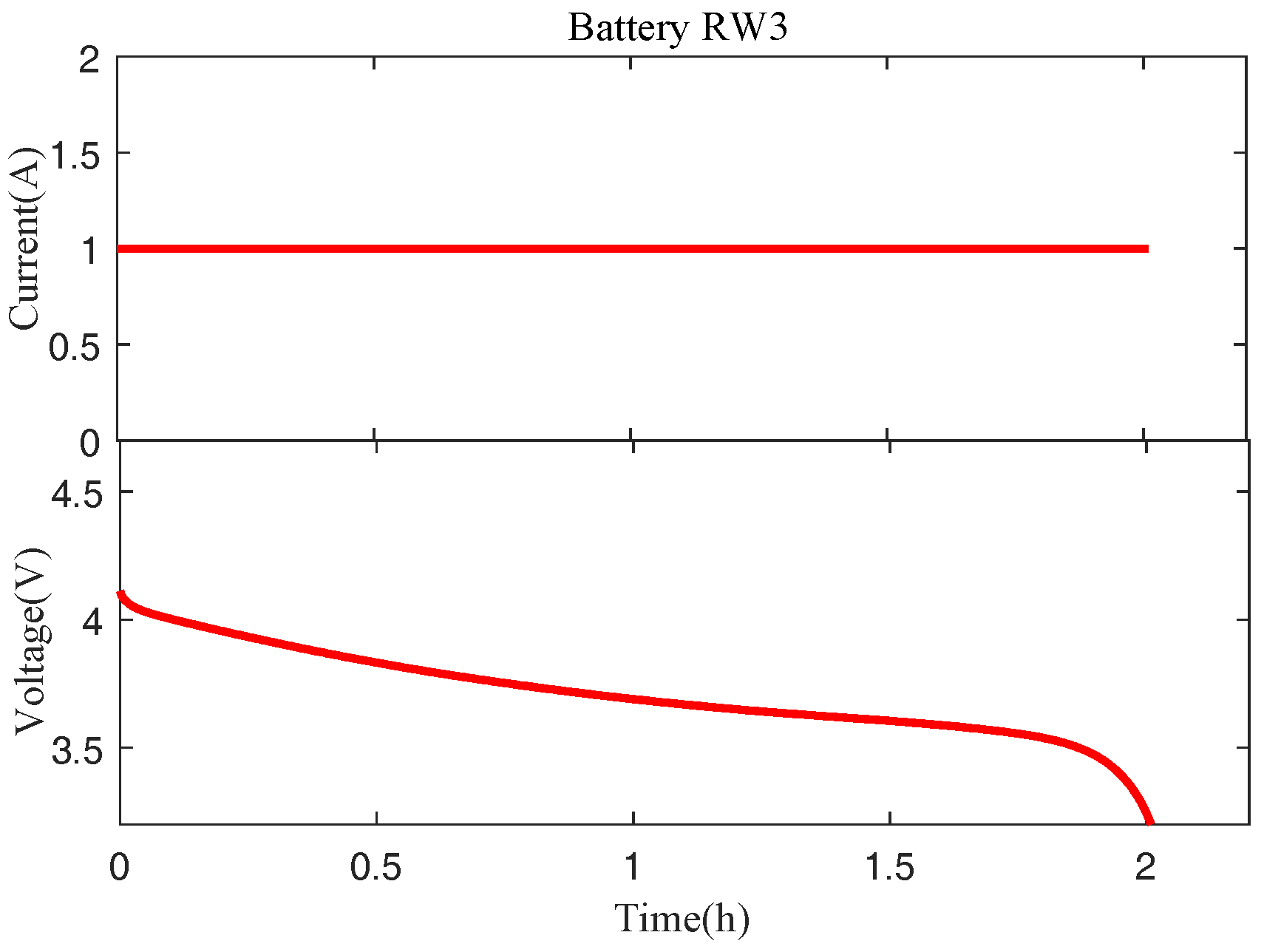
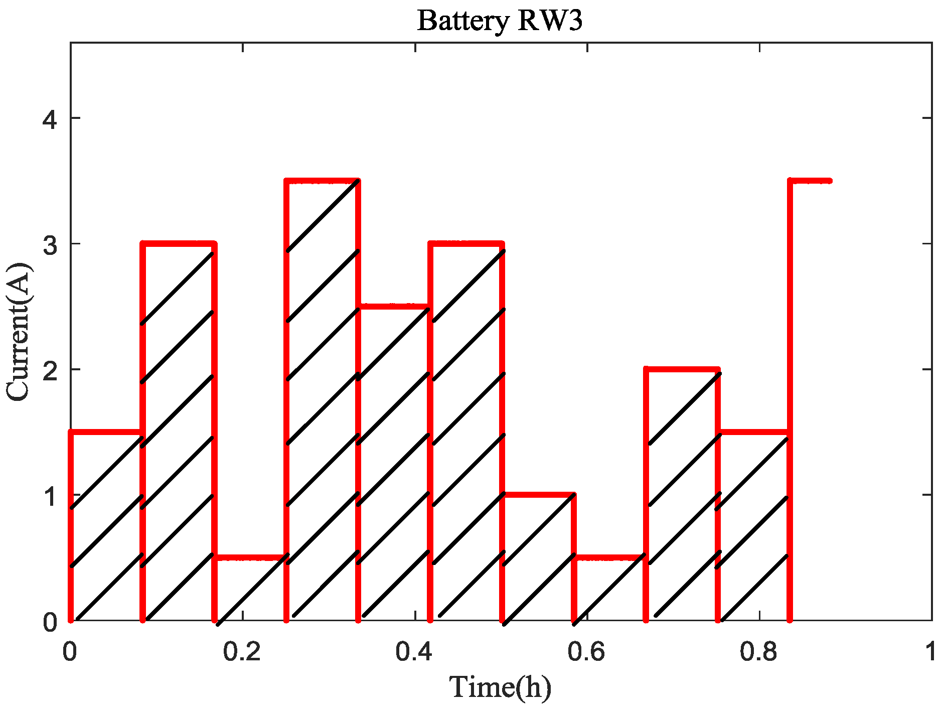
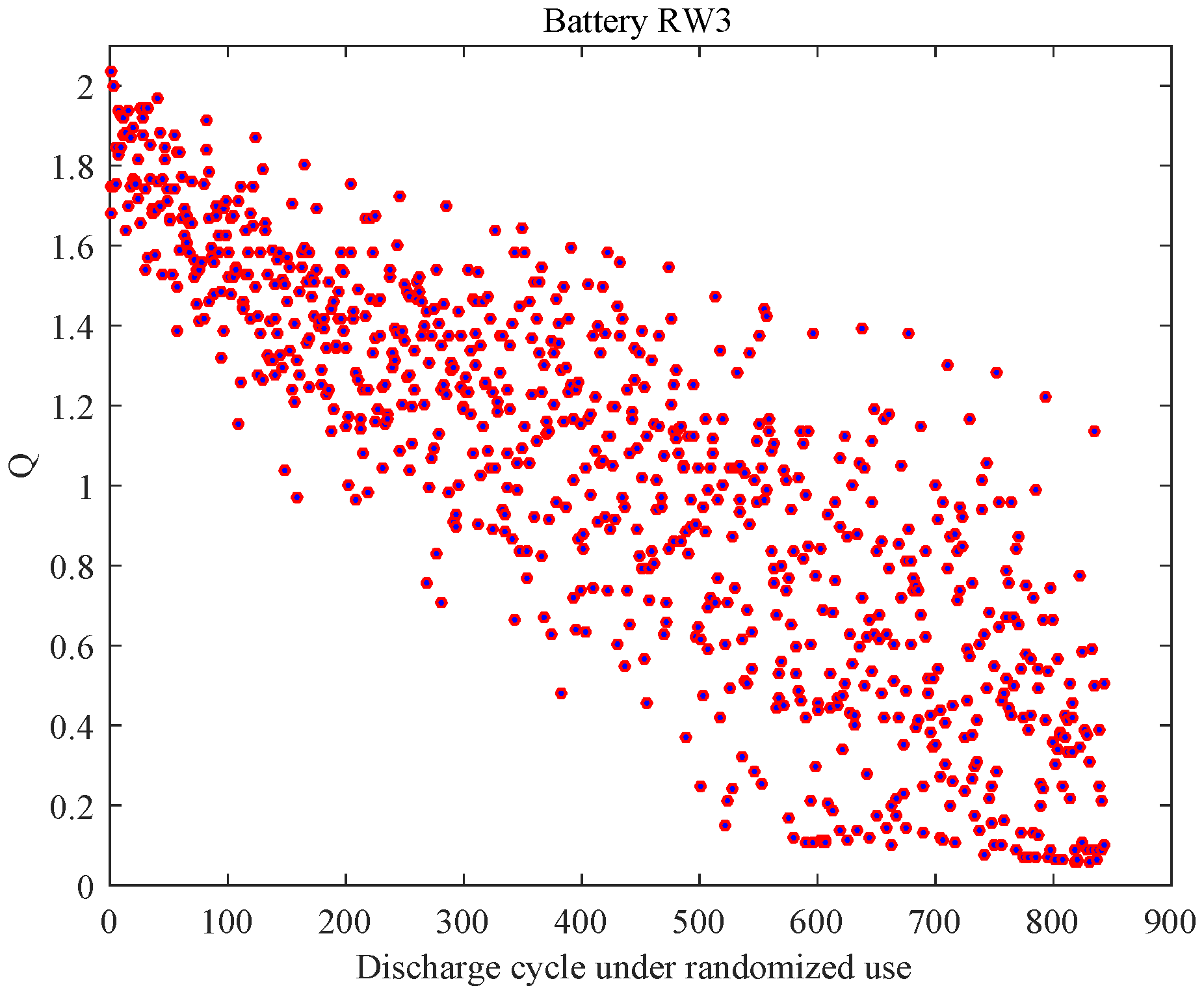
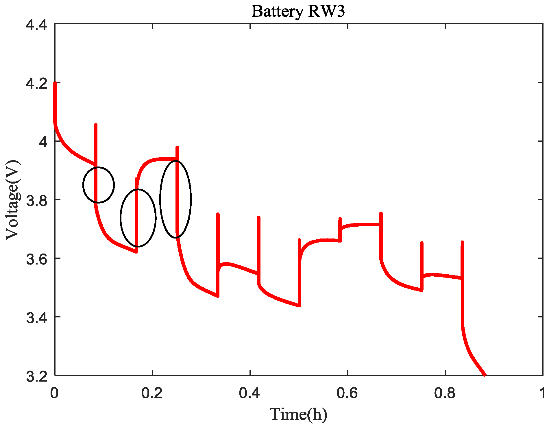
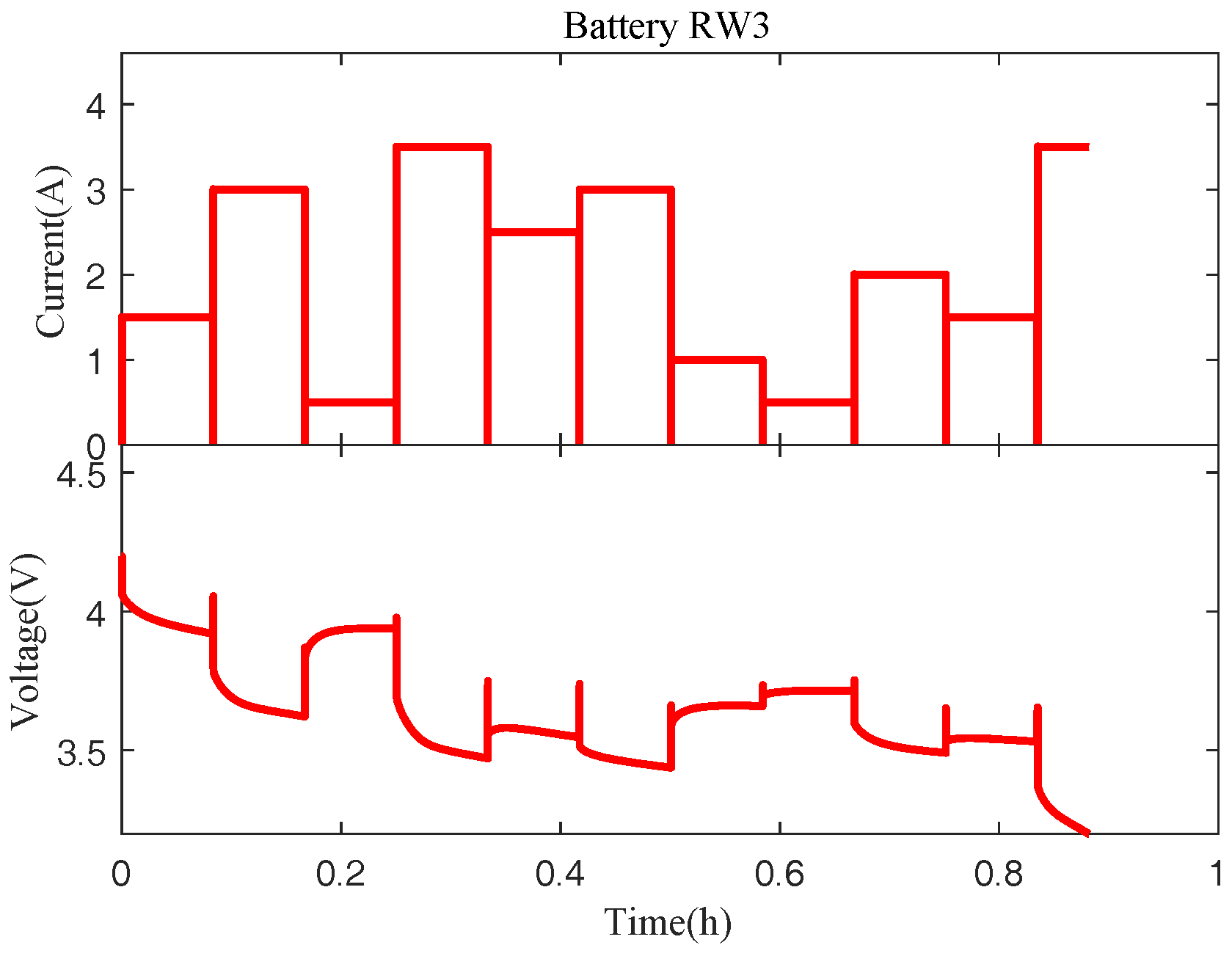
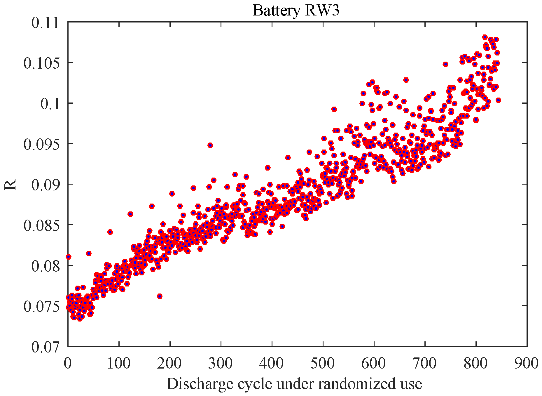
It can be noted that most of the existing literature mainly focuses on improving SOH estimation algorithms by using direct SOH indicators such as the battery’s capacity and internal resistance, while only a little attention has been paid to finding indirect health indicators (HIs) for SOH estimation, such as voltage and current, which can be easily measured during the usage of the battery. In fact, when lithium-ion batteries are used in electronic equipment, the battery’s capacity and internal resistance are very difficult to measure via existing sensors. Moreover, these quantities can only be used under constant loading conditions, which occur much less frequently in real practice. Therefore, it is necessary to find indirect HIs under randomized use of the battery for the online estimation of the SOH.

Among these limited works that have extracted indirect HIs for SOH estimation of lithium-ion batteries, two different approaches are used. One is analyzing HIs under a constant discharge process, and the other is achieved under a constant charge process. For example, Saha et al. [19] used the battery’s impedance as the HI for the SOH of battery, and Tong et al. [20] considered the open-circuit voltage, both under the circumstances of constant discharge. Moreover, Liu et al. [21] discovered that the time interval of equal discharging voltage difference in each discharge cycle can be used as a HI to represent the capacity degradation; Li et al. [22] used the temperature-change rate as the battery’s HI. For the HIs extracted under a constant charge process, some contributions are worthy of attention. For example, Wu et al. [23] selected the velocity and the arclength curvature of the charge curve as the HI, and then the group method of data handling was employed to estimate the SOH of the battery.

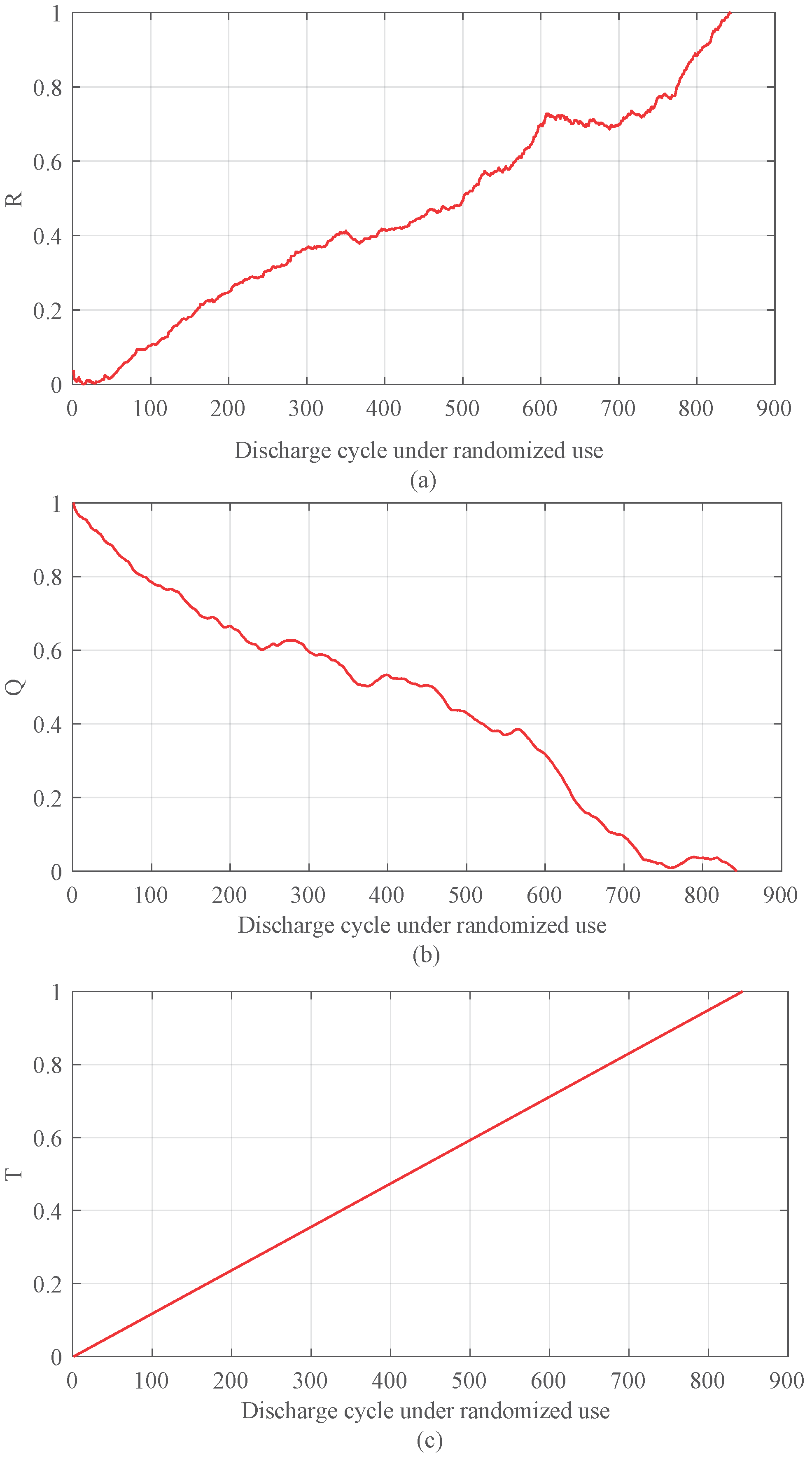
All the above HIs are extracted under a constant discharge cycle or constant charge cycle [24]. No contribution has been made to find indirect HIs for a battery’s SOH estimation under randomized loading conditions. However, in real engineering practice, a randomized loading condition is indeed the general situation. Therefore, in this paper, we dedicate efforts to extracting some indirect HIs for batteries’ SOH estimation under randomized loading conditions. For this purpose, we first explore HIs that can be easily obtained from the online condition-monitoring of the battery’s voltage and current, and we then develop a model based on an elastic net to build the linkage between these HIs and the battery’s SOH, considering the usually existing redundancies between the HIs. To our knowledge, we are the first to successfully build up indirect HIs to represent the battery’s health status under randomized use. In order to improve the online accuracy of the SOH estimation, we apply a particle filter (PF) to automatically update the model with possible available measurements of the true SOH.

The rest of this paper is organized as follows: Section 2 details the HI extraction. In Section 3, the relation between the HIs and capacity is constructed using the elastic net method. In Section 4, the PF is used to update the model with the new data, and the capacity of the batteries is predicted with the updated model. Finally, conclusions of the results as well as further work are given in Section 5.

2. Health Indicator Extraction

To estimate the SOH of lithium-ion batteries online, we first need to find some indirect HIs that can be measured easily to represent the battery’s SOH. Most existing contributions devoted to indirect HI extraction have focused on the situations under constant discharge conditions. However, these HIs cannot be applied under randomized use. Therefore, in this section, we first extract these robust indirect HIs.

2.1. The Dataset

In order to present our proposed indirect HIs for batteries under randomized use, we use the data provided by the NASA Ames Research Center for illustration [25]. In this dataset, a set of four 18,650 Li-ion batteries (identified as RW3, RW4, RW5 and RW6) were continuously operated by repeatedly charging them to 4.2 V and then discharging them to 3.2 V using a randomized sequence of discharging currents between 0.5 and 4 A. The sequence of discharging currents in the discharge process mimicked randomized use in real practice. Here, this type of discharging profile is referred to as random walk (RW) discharging. In order to know the true SOH of the aging battery, after every 50 RW discharging cycles, a series of reference charging and discharging cycles were performed. In these cycles, the battery was firstly fully charged to 4.2 V, then it rested for 20 min, and finally it was loaded at 1 A for 10 min. Every time, two continuous reference cycles were executed, and the capacity of each reference cycle was measured. The mean of the two capacities was considered as the true SOH at this moment. Figure 1 shows the whole process of the discharging and charging cycles. Figure 2 shows the true degrading trend of the capacity of every reference cycle in battery RW3.

The RW discharging and reference discharging cycles were carried out alternatively until the battery’s SOH reached the failure threshold. In each discharging cycle, the battery’s voltage and current were measured every 10 s. As shown in Figure 3, the battery’s voltage generally decreased with time, and it could be measured easily during the discharge. The battery’s current represents the load on battery, which was constant during reference discharging cycles and random during RW discharging cycles. From Figure 3, we can also observe that when the load was constant, the voltage trajectory decreased in a very clear way, from which indirect HIs could be easily extracted. For example, in [21], the time interval of an equal discharging voltage difference in each discharge cycle was decreased very clearly as the battery aged, which can be used as an indirect HI for SOH estimation. However, when the load is random, the voltage trajectory can be very irregular. See Figure 4, for instance. No contribution has been made to the extraction of indirect HIs under the situation of randomized load.

2.2. HI Extraction

In this paper, we define the battery SOH as follows [26]:

$$SOH=\frac{C_k}{C_0}\times 100\%$$

(1)

where $C_k$ is the battery’s capacity of the kth cycle, and $C_0$ is the rated capacity, which is known in advance.

Equation (1) indicates that, to estimate the battery SOH of the kth cycle, it is equivalent to estimate the capacity with the known rated capacity $C_k$. However, in real applications, such as in electric vehicles and satellites, measuring the battery’s capacity is difficult for current sensors. Therefore, some researchers have tried to find indirect HIs to represent the battery’s SOH, but their efforts have only been confined to the situation of constant loading conditions. In fact, lithium-ion batteries are usually used under randomized loading conditions; thus in this paper, we extract HIs for randomized loading situations in order to provide an efficient and accurate SOH estimation approach to meet practical requirements. In the following, we use the dataset described in Section 2.1 to illustrate our HI extraction under randomized use.

2.2.1. Charge Capacity

Generally, when the battery ages, its charge storage capacity decreases [27]. The storage capacity can be calculated using the current measured during each discharge cycle. This is the integration of the current of one cycle, as shown in Figure 5.

Therefore, the HI related to storage capacity for the kth cycle, denoted by $Q_k$, can be expressed as

$$Q_k=\underset{0}{\overset{t_k}{\int }}{i}_k(\tau )d\tau$$

(2)

where $i_k$($\tau$) is the current measured at the time $\tau$ in the kth cycle, which can be different at different $\tau$ according to the randomized loading condition; $t_k$ denotes the whole discharge time of the kth cycle.

Figure 6 shows the results of $Q_k$ for battery RW3 for the whole 844 discharge cycles under randomized use in the experiment. The trend of $Q_k$ is clearly degrading, which supports that $Q_k$ might be able to be linked to the battery’s SOH to a certain extent, as they are both reasonable representations of the battery’s degradation.

2.2.2. Internal Resistance

The second HI is the internal resistance, which is also extracted in the discharge cycle under randomized use. As the battery ages, its internal resistance generally increases [28]. Therefore, inspired by this idea, we consider a HI related to the internal resistance. In Figure 4, it can be observed that when there is a step change in the current, there will also be a step change in the voltage. The step change is marked more clearly in Figure 7. Therefore, we can use $R=\frac{\Delta U}{\Delta I}$ as the approximate internal resistance at the step-change time, where $\Delta I$ represents the step change of the current and $\Delta U$ represents the corresponding step change of the voltage. For each discharge cycle, there are several step changes for the current; thus we consider the mean value of all R as the HI, which is calculated by

$$R_k=\frac{1}{n}\sum _{i=1}^n\frac{\Delta U_i}{\Delta I_i}$$

(3)

where $R_k$ is the HI related to the internal resistance for the kth cycle, and n is the number of step changes in the kth cycle.

Figure 8 shows the results of $R_k$ for battery RW3 for the whole 844 discharge cycles under randomized use in the experiment. The trend of $R_k$ has a clear upward tendency, which is to be expected and may be able to be linked to the battery’s SOH.

2.2.3. Number of Cycles

In the experiment, when we obtained a new group of full discharge cycle and charge cycle, we increased the cycle counter; the value of the cycle counter is called the number of cycles in the following part. We notice that the charge capacity and internal resistance showed clear increasing or decreasing trend as the battery aged; the number of cycles that a battery had been going through also had the same characteristic. It is natural to consider the number of cycles as an indirect HI, for the battery degrades as the number of cycles increases. We demonstrate in the following sections that introducing the number of cycles is necessary to improve the accuracy of the SOH estimation.

2.2.4. HI Refinement

The three indirect HIs extracted for SOH estimation are summarized in

Table 2. Three extracted health indicators (HIs) for SOH estimation.

Extracted HI	Descriptions
$Q_k$	The estimated charge storage for the kth cycle
$R_k$	The estimated internal resistance for the kth cycle
$T_k$	The number of cycles up to the kth cycle

. We notice from Figure 5 and Figure 7 that the HIs extracted from the data contained many random errors. Thus, we applied the exponentially weighted moving average (EWMA) method [29] to refine those HIs. Using EWMA, the value of the current HI is a weighted average of several previous values of the HI. Supposing $Q=\left\{Q_1,Q_2,\dots ,Q_N\right\}$, $R=\left\{R_1,R_2,\dots ,R_N\right\}$, and $T=\left\{T_1,T_2,\dots ,T_N\right\}$ are the values of the HIs obtained up to the Nth cycle, then the refinements of $Q_k$ and $R_k$, $k\in \left\{1,2,\dots ,N\right\}$, are found using the following equation:

$$\begin{array}{c}{Q}_k^{*}=\phi Q_k+(1-\phi )Q_{k-1}^{*}\hfill \\ R_k^{*}=\phi R_k+(1-\phi )R_{k-1}^{*}\hfill \end{array}$$

(4)

where $\phi$ is the weight factor, which decays exponentially with k.

Moreover, in order to eliminate the large value difference between different HIs, we use min-max normalization [30] to make sure all HIs belong to the same interval, [0, 1]. The transformation function is

$$\begin{array}{c}{\tilde{Q}}_k^{*}=\frac{Q_k^{*}-min(Q^{*})}{max(Q^{*})-min(Q^{*})}\hfill \\ {\tilde{R}}_k^{*}=\frac{R_k^{*}-min(R^{*})}{max(R^{*})-min(R^{*})}\hfill \\ {\tilde{T}}_k^{*}=\frac{T_k-min(T)}{max(T)-min(T)}\hfill \end{array}$$

(5)

Using the above refinement, the HIs extracted for battery RW3 for the whole 844 discharge cycles under randomized use are shown in Figure 9. From Figure 9, we can see that as the battery aged, ${\tilde{Q}}_k^{*}$ decreased, and ${\tilde{R}}_k^{*}$ and ${\tilde{T}}_k^{*}$ increased, all following a clear trend. These have a specific physical significance to support that they are closely related to the degradation of the battery, which makes them qualified for estimating the battery’s SOH. They are based on the voltage, the current and the number of cycles the battery has been through, which indicates they can be easily obtained and calculated during the battery’s operation. In the next section, we use these HIs to build the relationship between the indirect HIs and the battery’s SOH.

3. State-of-Health Modeling Using Indirect Health Indicators

After the extraction of indirect HIs, a quantitative model that describes the relationship between these HIs and the battery’s SOH should be developed. We consider that the SOH and these HIs follow a linear regression model, that is, as follows:

$${\widehat{S}}_k=a\times {\tilde{Q}}_k^{*}+b\times {\tilde{R}}_k^{*}+c\times {\tilde{T}}_k^{*}+d+\epsilon ={\mathbf{F}}_k\mathit{\beta }+\epsilon$$

(6)

where ${\widehat{S}}_k$ is the estimated battery’s SOH for the kth cycle, $\mathit{\beta }={[a,b,c,d]}^T$ is the model coefficient vector we have to estimate, ${\mathbf{F}}_k=[{\tilde{Q}}_k^{*},{\tilde{R}}_k^{*},{\tilde{T}}_k^{*},1]$, and $\epsilon$ is the error term. We assume the errors are identically and independent distributed with a zero mean and finite variance ${\sigma }^2$, which means $\epsilon \sim N(0,{\sigma }^2)$.

Considering possible multi-collinearity among the HIs, we apply the elastic net method to estimate the model coefficients. Proposed by Zou and Zhang [31], the elastic net is a regularized regression method that linearly combines the L1 and L2 penalties of the lasso and ridge methods. Compared to the Lasso, which tends to select one variable from a group of highly correlated variables, the elastic net tends to distribute different weights to different variables. Therefore, the elastic net removes the limitation on the number of selected variables and stabilizes the L1 regularization path.

To demonstrate the necessity of using the elastic net to construct our model, we need to prove the existence of multi-collinearity among the HIs. Firstly, we use Pearson’s correlation coefficient [32] between two different HIs to find whether these HIs are linearly correlated. The results are shown in

Table 3. Results of Pearson’s correlation coefficient between HIs.

	Q	R	T
Q	1	−0.9845	−0.9872
R	−0.9845	1	0.9912
T	−0.9872	0.9912	1

. Table 3 indicates that there is a remarkable linear correlation between these HIs. Then, we use the variance inflation factor (VIF) [33] to quantify the severity of multi-collinearity. This indicates high multi-collinearity when its value is greater than 10. The result of VIF was 100, which is an indicator of high multi-collinearity. The existence of multi-collinearity forces us to use methods that can alleviate the influence of multi-collinearity. This is why we chose the elastic net method.

The elastic net loss function defined as

$$L({\lambda }_1,{\lambda }_2,\mathit{\beta })=\sum _{k=1}^N|S_k-{\mathbf{F}}_k{\mathit{\beta }|}^2+{\lambda }_1{|\mathit{\beta }|}^2+{\lambda }_2{|\mathit{\beta }|}_1$$

(7)

where $S_k$ is the battery’s true SOH at the kth cycle, ${\lambda }_1$ and ${\lambda }_2$ are user-defined parameters, and

$$\begin{array}{c}{|\mathit{\beta }|}^2=a^2+b^2+c^2+d^2\hfill \\ {|\mathit{\beta }|}_1=|a|+|b|+|c|+|d|\hfill \end{array}$$

(8)

We define $\alpha ={\lambda }_2/({\lambda }_1+{\lambda }_2)$; then our target is to solve the following optimization problem:

$$MinL(\alpha ,\mathit{\beta })=\sum _{k=1}^N|S_k-{\mathbf{F}}_k{\mathit{\beta }|}^2+{\alpha |\mathit{\beta }|}^2+(1-\alpha ){|\mathit{\beta }|}_1$$

(9)

where the function ${(1-\alpha )|\mathit{\beta }|}_1+\alpha {|\mathit{\beta }|}^2$ is called the elastic net penalty, which is a convex combination of the lasso and ridge penalty. When $\alpha =1$, the elastic net becomes simple ridge regression, and when $\alpha =0$, the elastic net becomes simple lasso regression. In this paper, we consider $0<\alpha <1$ to combine advantages of both regression methods.

The estimates of model coefficients are obtained by

$$\widehat{\mathit{\beta }}=arg\underset{\mathit{\beta }}{min}\sum _{k=1}^N|S_k-{\mathbf{F}}_k{\mathit{\beta }|}^2+{(1-\alpha )|\mathit{\beta }|}_1+\alpha {|\mathit{\beta }|}^2$$

(10)

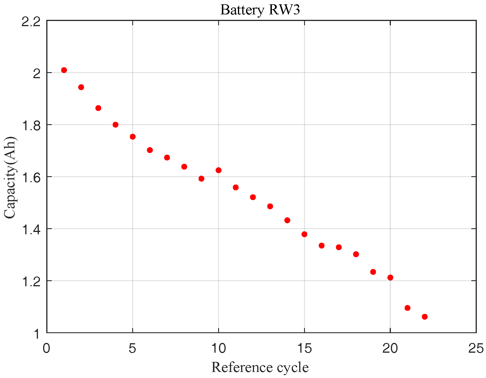
After obtaining the estimate of model coefficient $\widehat{\mathit{\beta }}$ by the elastic net method, the battery’s SOH can be estimated using the values of $Q_k$, $R_k$ and $T_k$. We used the dataset described in Section 2.1 to estimate the model coefficient $\widehat{\mathit{\beta }}$ for each battery and to demonstrate the effectiveness of the model. The estimation results are shown in

Table 4. Estimates of model coefficients for each battery.

Battery	a	b	c	d
RW3	−0.1463	0.1229	−0.1575	0.8505
RW4	−0.1220	0.1112	−0.1558	0.8638
RW5	−0.1285	0.1071	−0.1517	0.8800

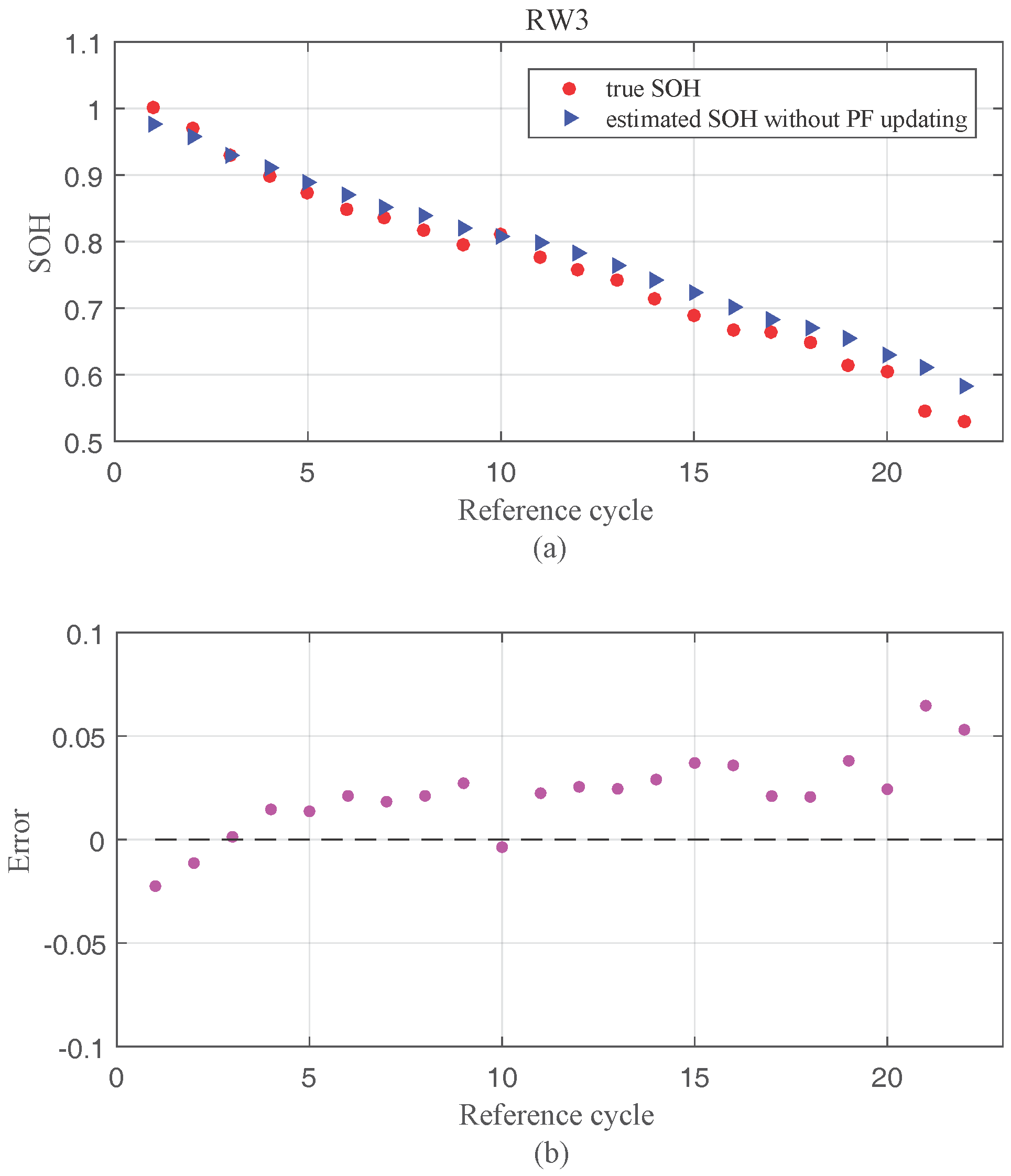
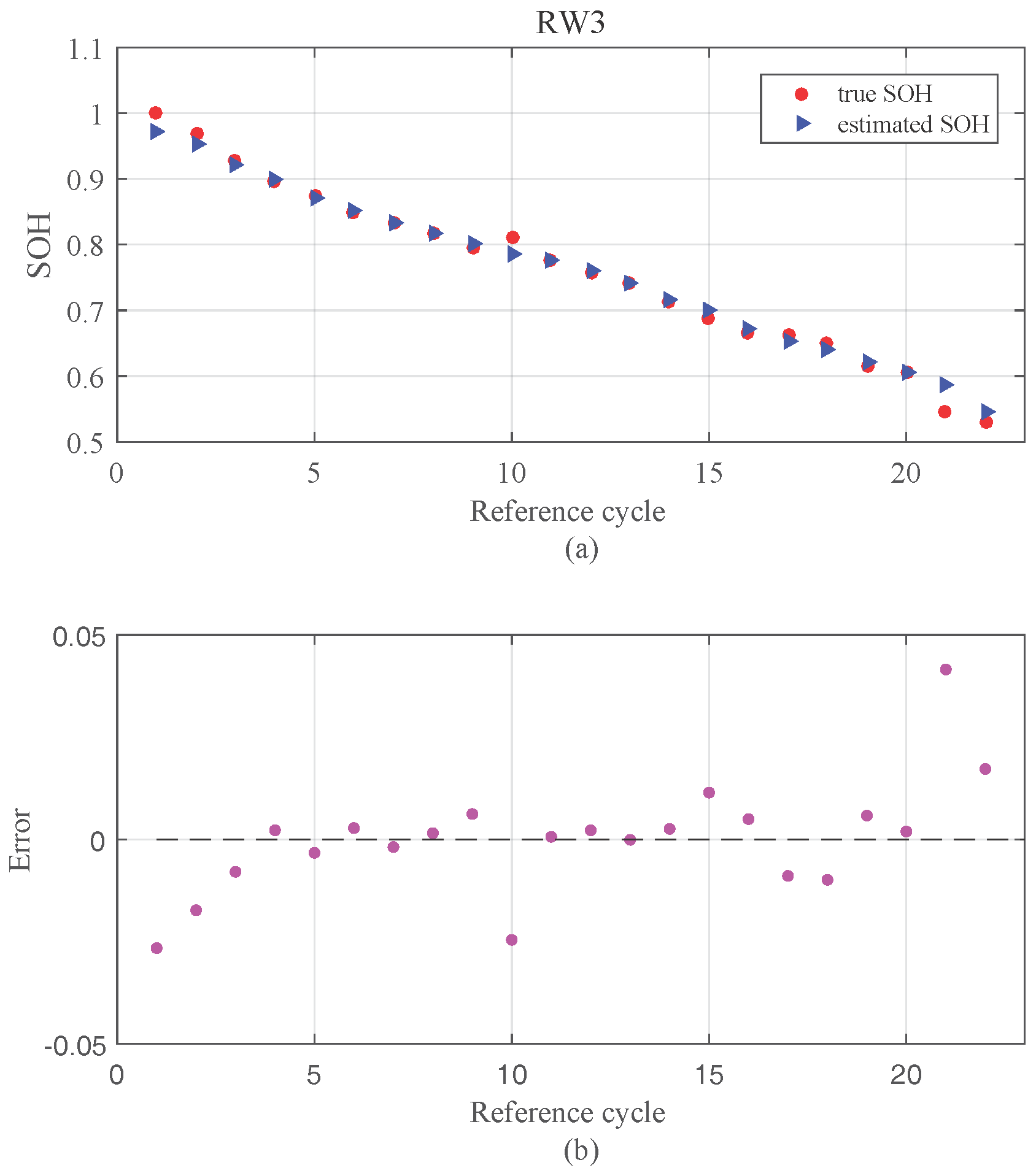
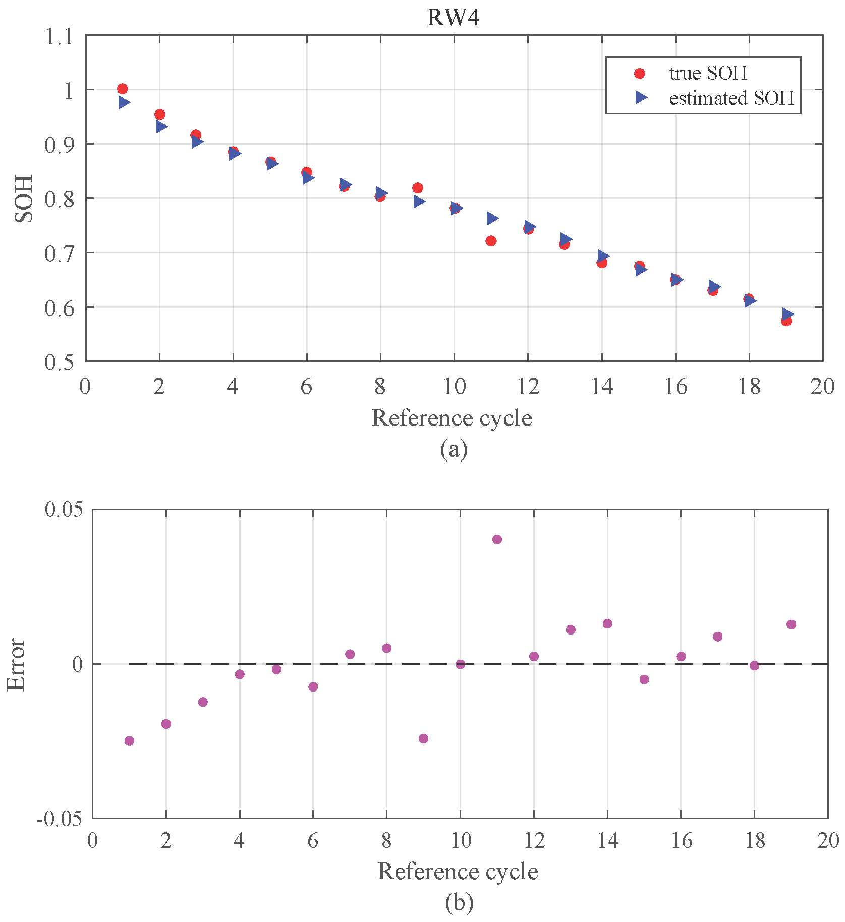
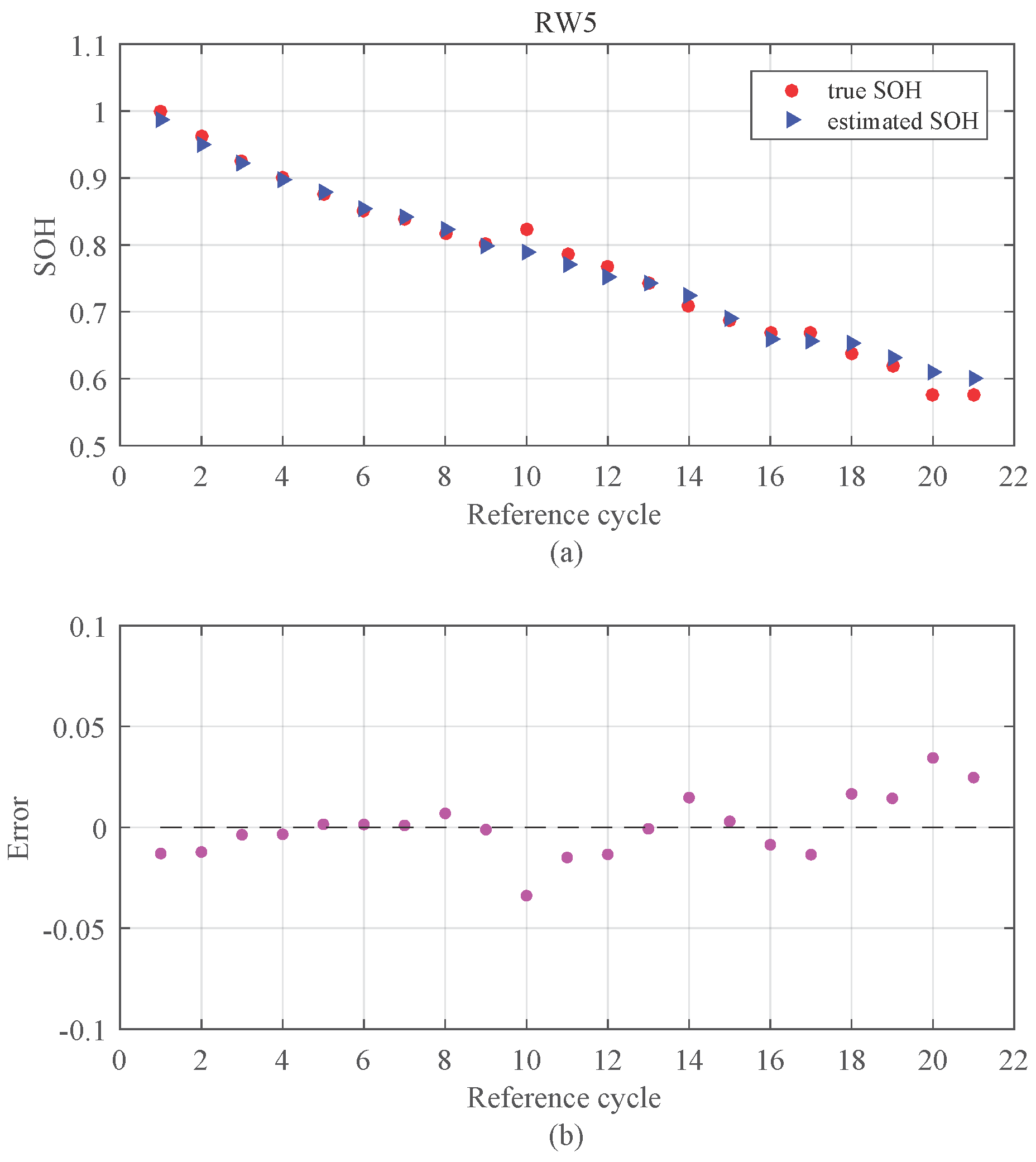
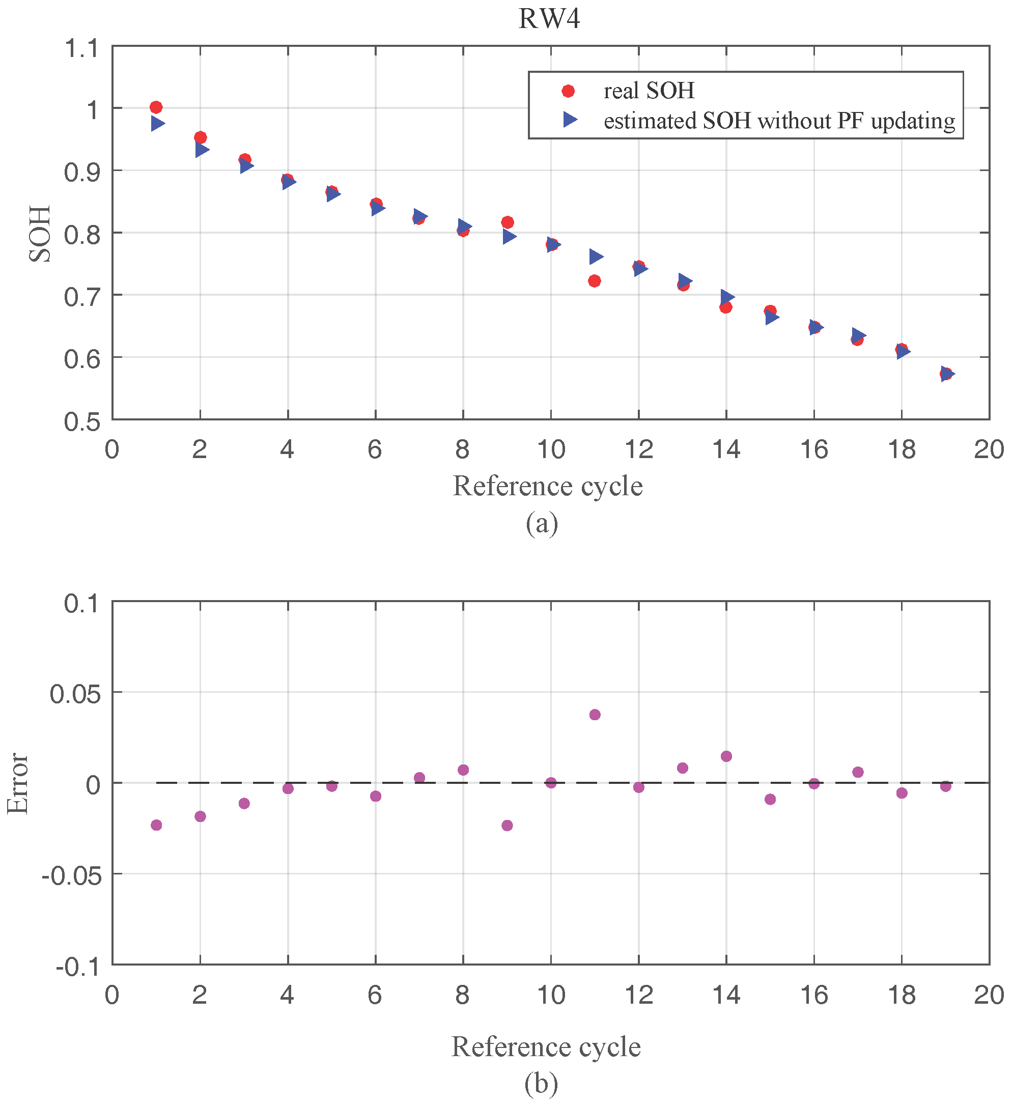
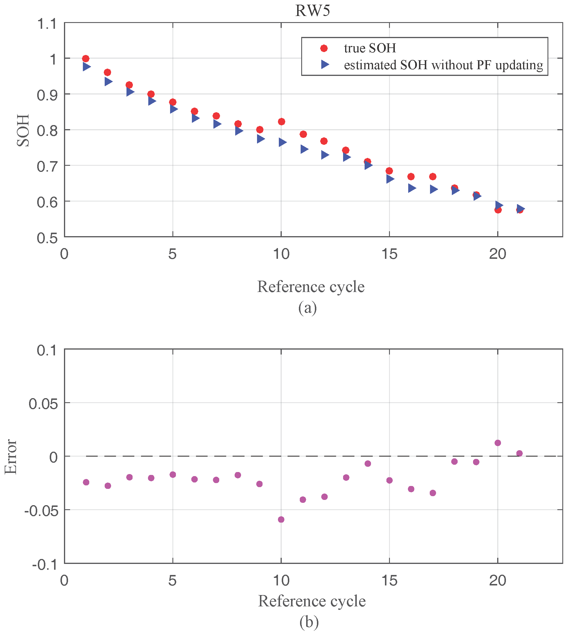
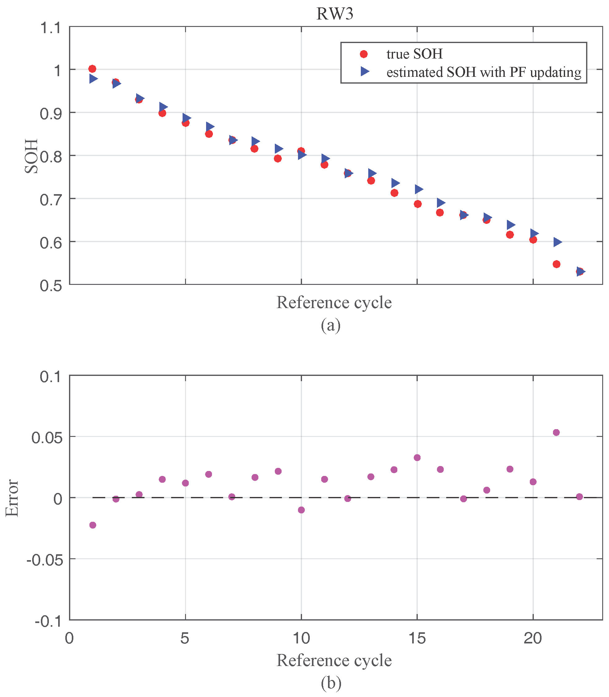
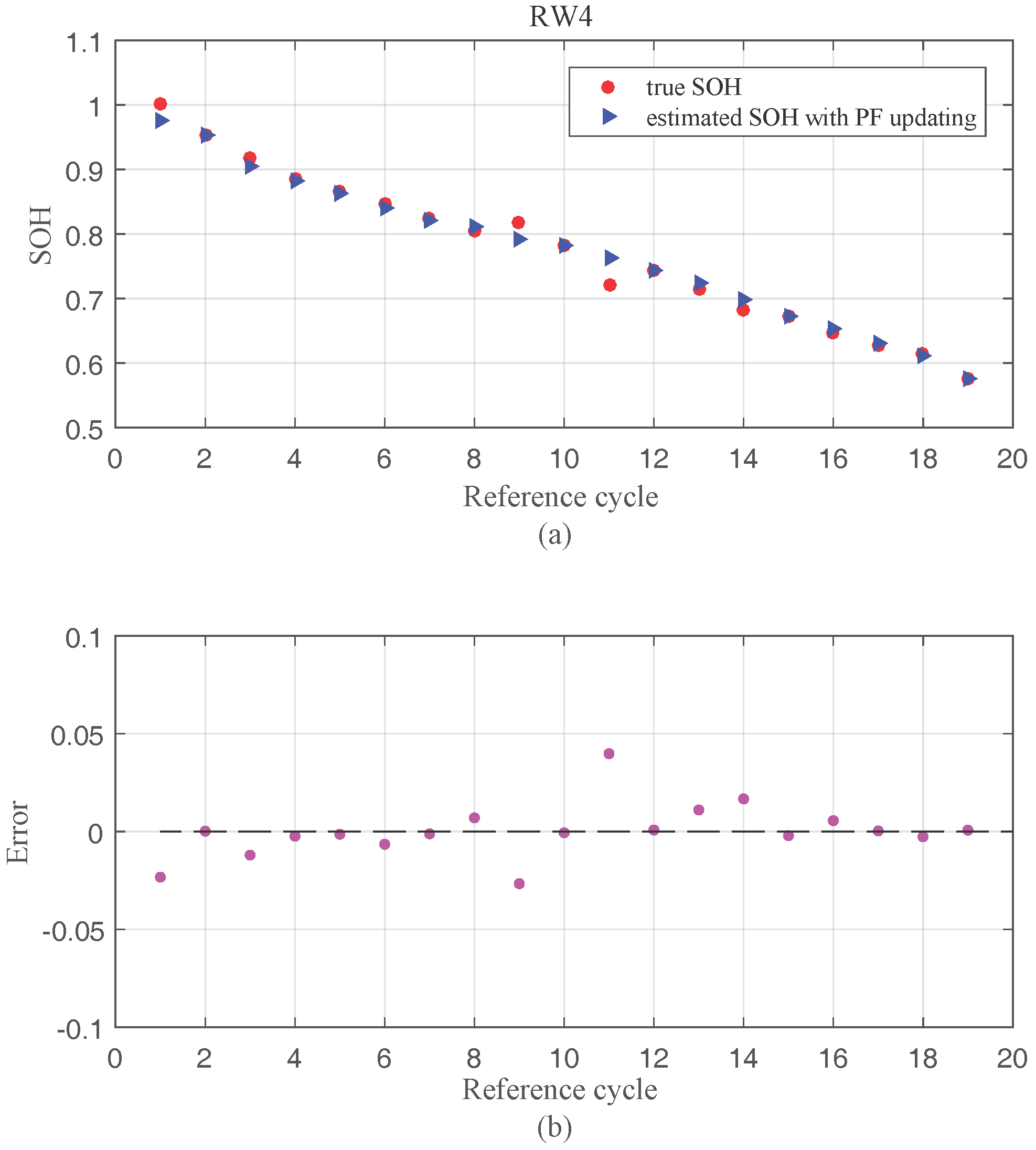
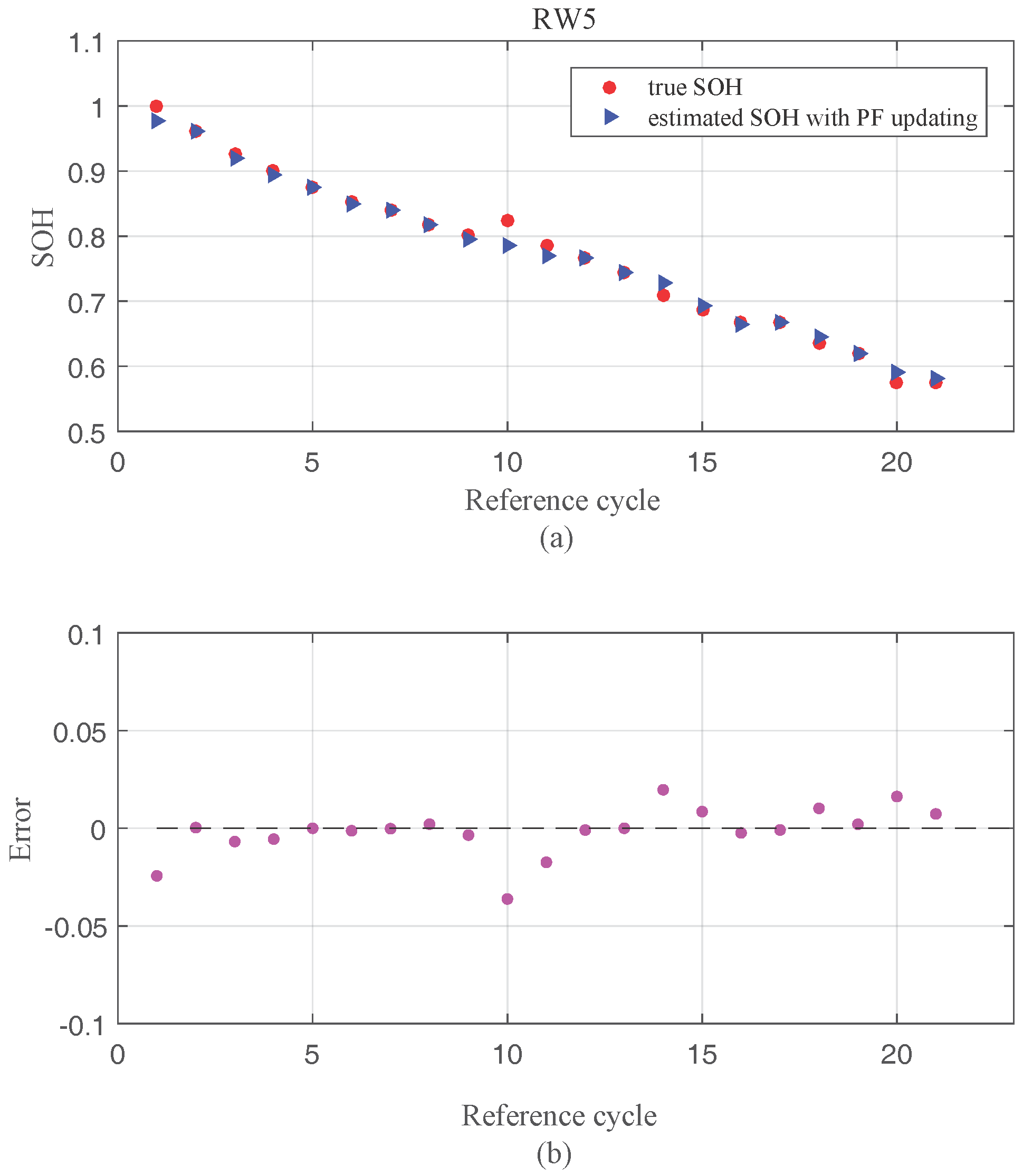
. Using these estimates, we were able to estimate the SOH of each battery at each cycle time. Figure 10, Figure 11 and Figure 12 show the SOH estimation results for each battery, accompanied with the true SOH measured in the reference cycle. The results support that the model is effective to describe the relationship between HIs and the battery’s SOH.

4. Online State-of-Health Estimation Using Particle Filter

To achieve online SOH estimation of lithium-ion batteries, we use PF to update the model coefficients. When new measurements of the voltage, current and number of cycles are available, the PF can automatically update the model coefficient $\mathit{\beta }={[a,b,c,d]}^T$ in order to make the SOH estimation more accurate.

4.1. The Method

The PF is a Monte Carlo-based computational tool that is particularly useful for Bayesian-framed prognostics of nonlinear and/or non-Gaussian processes [34]. In order to approximate the marginal distribution, the PF generates a large number of random particles and estimates the posterior density function (PDF) through accumulating these particles with associated weights.

The PF considers a dynamic system to be represented by a state transition equation and an observation equation, which are given by

$$\begin{array}{c}\mathrm{State}\mathrm{transition}\mathrm{equation}:{\mathbf{X}}_k=g\left[{\mathbf{X}}_{k-1},{\mathbf{U}}_k\right]\hfill \\ \mathrm{Observation}\mathrm{equation}:{\mathbf{Y}}_k=h\left[{\mathbf{X}}_k,{\mathbf{V}}_k\right]\hfill \end{array}$$

(11)

where $\mathbf{X}$ is the state vector representing the true state of the system; $\mathbf{Y}$ is the measurement vector documenting the observations acquired by sensors; g and h denote respectively the state transition function and the observation function, which can be nonlinear; $\mathbf{U}$ denotes the progress noise and $\mathbf{V}$ denotes the measurement noise; and k is the time index.

Then, the posterior PDF of ${\mathbf{X}}_k$ given all available measurements ${\mathbf{Y}}_{0:k}$ up to time k can be approximated using a set of weighted particles $\left\{\left({\omega }_k^i,{\mathbf{X}}_k^i\right):i=1,\dots ,M\right\}$, that is, as follows:

$$\begin{array}{c}Pr\left({\mathbf{X}}_k|{\mathbf{Y}}_{0:k}\right)\approx {\displaystyle \sum _{i=1}^M}{\omega }_k^i\delta \left({\mathbf{X}}_k-{\mathbf{X}}_k^i\right)\hfill \\ {\displaystyle \sum _{i=1}^M}{\omega }_k^i=1\hfill \end{array}$$

(12)

where ${\mathbf{X}}_k^i$ denotes the ith particle and ${\omega }_k^i$ is its associated importance weight; $\delta$ is the Dirac delta function.

However, it is often impossible to sample directly from the true posterior density $Pr\left({\mathbf{X}}_k|{\mathbf{Y}}_{0:k}\right)$. Therefore, a simpler distribution is introduced, denoted as the importance distribution, $q\left({\mathbf{X}}_k|{\mathbf{X}}_{0:k-1},{\mathbf{Y}}_{1:k}\right)$. Then, the weight ${\omega }_{k+1}^i$ is updated by

$${\omega }_{k+1}^i={\omega }_k^i\frac{Pr\left({\mathbf{Y}}_k|{\mathbf{X}}_k\right)Pr\left({\mathbf{X}}_k|{\mathbf{X}}_{k-1}\right)}{q\left({\mathbf{X}}_k|{\mathbf{X}}_{0:k-1},{\mathbf{Y}}_{1:k}\right)}$$

(13)

In the standard PF, $q\left({\mathbf{X}}_k|{\mathbf{X}}_{0:k-1},{\mathbf{Y}}_{1:k}\right)$ is defined as $Pr\left({\mathbf{X}}_k|{\mathbf{X}}_{k-1}\right)$, and therefore the weight ${\omega }_{k+1}^i$ is normalized using the following formula:

$${\omega }_{k+1}^i={\omega }_{k+1}^i/\sum _{i=1}^M{\omega }_{k+1}^i$$

(14)

In our SOH estimation problem, we consider the model coefficients $\left\{a,b,c,d\right\}$ as state variables in the state transition equation, and they follow a Gaussian RW process. Then, with the empirical model of Equation (6) we have established for the SOH and indirect HIs, we have the state transition equation:

$$\begin{array}{c}{a}_k=a_{k-1}+{u_{1,}}_{k-1},{u_1}_{,k-1}\sim N(0,{\sigma }_1)\hfill \\ b_k=b_{k-1}+{u_2}_{,k-1},{u_2}_{,k-1}\sim N(0,{\sigma }_2)\hfill \\ c_k=c_{k-1}+{u_3}_{,k-1},{u_3}_{,k-1}\sim N(0,{\sigma }_3)\hfill \\ d_k=d_{k-1}+u_{4,k-1},{u_4}_{,k-1}\sim N(0,{\sigma }_4)\hfill \\ {\widehat{S}}_k=a_{k-1}\times {\tilde{Q}}_k^{*}+b_{k-1}\times {\tilde{R}}_k^{*}+c_{k-1}\times {\tilde{T}}_k^{*}+d_{k-1}+{u_5}_{,k},u_{5,k}\sim N(0,{\sigma }_5)\hfill \end{array}$$

(15)

and the observation equation:

$$S_k={\widehat{S}}_k+v_k,v_k\sim N(0,{\sigma }_6)$$

(16)

where $u_{1,k-1}$, $u_{2,k-1}$, $u_{3,k-1}$, $u_{4,k-1}$, and $u_{5,k-1}$ are five independent progress noises, which obey zero-mean Gaussian distribution; $v_k$ is the measurement noise, which also obeys the zero-mean Gaussian distribution. In this paper, according to the results in Table 4, we notice that the order of the variables in the state transition is of 0.1. Therefore, the process noise is set as $u_{i,k}=0.0001\forall i\in [1,5]$; and the observation noise is set as $v_k=0.0001$.

Using the PF, we are able update the value of $\left\{a_k,b_k,c_k,d_k\right\}$ given the latest measured SOH $S_k$. Then, the updated $\left\{a_k,b_k,c_k,d_k\right\}$ can be used to estimate the battery’s SOH at any future cycle (the $\tilde{k}$th cycle, $\tilde{k}>k$), when the values of these indirect HIs are available. It is given by

$${\widehat{S}}_{\tilde{k}}=a_k\times {\tilde{Q}}_{\tilde{k}}^{*}+b_k\times {\tilde{R}}_{\tilde{k}}^{*}+c_k\times {\tilde{T}}_{\tilde{k}}^{*}+d_k$$

(17)

4.2. Result and Analysis

We choose batteries RW3, RW4, and RW5 to demonstrate the effectiveness of our method. The method of cross-validation was employed, in which we used two batteries to train the model and used the remaining battery to test the SOH estimation method. For example, in the first experiment, the batteries RW3 and RW4 were used as the training batteries, and the battery RW5 was used as the testing battery. In this way, we performed three experiments. The initial model parameters estimated from the data of training batteries are listed in

Table 5. Initial model parameters.

Training Battery	Testing Battery	a	b	c	d
RW4, RW5	RW3	−0.1202	0.1076	−0.1672	0.8699
RW3, RW5	RW4	−0.0946	0.1400	−0.1694	0.9829
RW3, RW4	RW5	−0.1276	0.1150	−0.1553	0.8606

.

To quantitatively evaluate the performance of the SOH estimation, two evaluation criteria were used:

• The root-mean-square error (RMSE):

  $$RMSE=\sqrt{\frac{1}{N}\sum _{k=1}^N{(S_k-{\widehat{S}}_k)}^2}$$

  (18)
• The fitness degree:

  $$R^2=1-\frac{{\displaystyle \sum _{k=1}^N}{(S_k-{\widehat{S}}_k)}^2}{{\displaystyle \sum _{k=1}^N}{(S_k-\overline{S})}^2}$$

  (19)

  where $S_k$ is the true SOH, ${\widehat{S}}_k$ is the estimated SOH, $\overline{S}$ is the mean value of all $S_k$, and N is the sample size.

The estimation results without PF updating are shown in Figure 13, Figure 14 and Figure 15. We can observe that nearly all errors were smaller than 0.05. The results are quite good. To improve the estimation accuracy, we used the PF to update the estimation results. We suppose that every five cycles we are able to obtain the true value of the SOH; then the model parameters can be updated by the PF every five cycles. The estimation results with PF updating are shown in Figure 16, Figure 17 and Figure 18.

These show that compared to the results without PF updating, the error can be reduced with the updating of model parameters. The detailed estimation results are shown in

Table 6. SOH estimation results.

Evaluation Critieria	RW3		RW4		RW5
	Without	With	Without	With	Without	With
	Update	Update	Update	Update	Update	Update
$RMSE$	0.0287	0.0194	0.0194	0.0136	0.0261	0.0123
$R^2$	0.9502	0.9773	0.9773	0.9866	0.9534	0.9896

. When there is no updating, we can still get a very good estimation result: the $RMSE$ was around 0.02, and the $R^2$ value was about 0.95. When the PF is used, a better estimation result can be obtained. The $RMSE$ was smaller than 0.02, and the $R^2$ was about 0.98. From the experimental results, we can expect that our proposed SOH estimation method will have a good performance in SOH online estimation for lithium-ion batteries under randomized use.

5. Conclusions

Timely estimating lithium-ion batteries’ SOH is very important for preventing disasters caused by battery failure. A general idea to estimate the SOH is through the measurement of the battery’s capacity. However, direct and simultaneous measurement of the battery’s capacity is not that easy in practice. Moreover, the battery is always running under randomized loading conditions, which makes the estimation even more difficult. Motivated by the above difficulties, this paper proposes an indirect SOH estimation method that relies on three indirect HIs that can be measured easily during the battery’s operation. The three indicators are extracted from the battery’s voltage, the current and the number of cycles the battery has been through, which are far easier to measure than the battery’s capacity. In order to build a quantitative relationship between the SOH and these indirect HIs, we propose a method based on an elastic net to develop an empirical model between them, considering the possible multi-collinearity between these HIs. Finally, to further improve the accuracy of SOH online estimation, we adopt the PF to automatically update the model when new capacity data are available. The experiment shows that our extracted indirect HIs are quite effective and our proposed SOH estimation method based on these HIs is accurate enough to support SOH estimation under randomized use in real practice.

In this paper, we have successfully applied our method to estimate the SOH of batteries under randomized use. However, there are some limitations, on which we will conduct research in the future. The data we used was obtained from a constant-temperature environment. Therefore, performing a validation with temperature consideration is necessary. In this paper, the PF was used to update the parameters in the model. Comparing the PF with other estimation schemes is necessary.

References

1. Nishi, Y. Lithium ion secondary batteries; past 10 years and the future. J. Power Sources 2001, 100, 101–106. [Google Scholar] [CrossRef]
2. Wang, D.; Miao, Q.; Pecht, M. Prognostics of lithium-ion batteries based on relevance vectors and a conditional three-parameter capacity degradation model. J. Power Sources 2013, 239, 253–264. [Google Scholar] [CrossRef]
3. Millner, A. Modeling Lithium Ion battery degradation in electric vehicles. In Proceedings of the 2010 IEEE Conference on Innovative Technologies for an Efficient and Reliable Electricity Supply (CITRES), Waltham, MA, USA, 27–29 September 2010; pp. 349–356. [Google Scholar]
4. Li, J.; Chao, L.; Wang, L.; Ge, T. Model-based method for estimating LiCoO2 battery state of health and behaviors. In Proceedings of the IEEE International Conference on Prognostics and Health Management, Ottawa, ON, Canada, 20–22 June 2016; pp. 1–4. [Google Scholar]
5. Samadi, M.F.; Alavi, S.M.M.; Saif, M. An electrochemical model-based particle filter approach for Lithium-ion battery estimation. In Proceedings of the 2012 IEEE 51st Annual Conference on Decision and Control (CDC), Maui, HI, USA, 10–13 December 2012. [Google Scholar]
6. Hu, C.; Youn, B.D.; Chung, J. A multiscale framework with extended Kalman filter for lithium-ion battery SOC and capacity estimation. Appl. Energy 2012, 92, 694–704. [Google Scholar] [CrossRef]
7. Saha, B.; Goebel, K. Modeling li-ion battery capacity depletion in a particle filtering framework. In Proceedings of the Annual Conference of the Prognostics and Health Management Society, San Diego, CA, USA, 27 September–1 October 2009; Volume 58, pp. 291–296. [Google Scholar]
8. Li, J.; Chao, L.; Wang, L.; Zhang, L.; Li, C. Remaining capacity estimation of li-ion batteries based on temperature sample entropy and particle filter. J. Power Sources 2014, 268, 895–903. [Google Scholar] [CrossRef]
9. Tran, N.T.; Khan, A.B.; Choi, W. State of charge and state of health estimation of agm vrla batteries by employing a dual extended kalman filter and an arx model for online parameter estimation. Energies 2017, 10, 137. [Google Scholar] [CrossRef]
10. Tao, L.; Ma, J.; Cheng, Y.; Noktehdan, A.; Chong, J.; Lu, C. A review of stochastic battery models and health management. Renew. Sustain. Energy Rev. 2017, 80, 716–732. [Google Scholar] [CrossRef]
11. Zhang, C.; Jiang, J.; Zhang, W.; Wang, Y.; Sharkh, S.M.; Xiong, R. A novel data-driven fast capacity estimation of spent electric vehicle lithium-ion batteries. Energies 2014, 7, 8076–8094. [Google Scholar] [CrossRef]
12. Rezvani, M.; Lee, S.; Lee, J. A Comparative Analysis of Techniques for Electric Vehicle Battery Prognostics and Health Management (PHM). SAE Tech. Pap. 2011, 7, 6492–6508. [Google Scholar]
13. He, Y.J.; Shen, J.N.; Shen, J.F.; Ma, Z.F. State of health estimation of lithium-ion batteries: A multiscale gaussian process regression modeling approach. AIChE J. 2015, 61, 1589–1600. [Google Scholar] [CrossRef]
14. Hu, C.; Jain, G.; Schmidt, C.; Strief, C.; Sullivan, M. Online estimation of lithium-ion battery capacity using sparse bayesian learning. J. Power Sources 2015, 289, 105–113. [Google Scholar] [CrossRef]
15. Dong, H.; Jin, X.; Lou, Y.; Wang, C. Lithium-ion battery state of health monitoring and remaining useful life prediction based on support vector regression-particle filter. J. Power Sources 2014, 271, 114–123. [Google Scholar] [CrossRef]
16. Li, F.; Xu, J. A new prognostics method for state of health estimation of lithium-ion batteries based on a mixture of gaussian process models and particle filter. Microelectron. Reliab. 2015, 55, 1035–1045. [Google Scholar] [CrossRef]
17. Saha, B.; Poll, S.; Goebel, K.; Christophersen, J. An integrated approach to battery health monitoring using bayesian regression and state estimation. In Proceedings of the 2007 IEEE Autotestcon, Baltimore, MD, USA, 17–20 September 2007; pp. 646–653. [Google Scholar]
18. Chaoui, H. State of charge and state of health estimation for lithium batteries using recurrent neural networks. IEEE Trans. Veh. Technol. 2017, 66, 8773–8783. [Google Scholar] [CrossRef]
19. Saha, B.; Goebel, K.; Poll, S. Prognostics methods for battery health monitoring using a Bayesian framework. IEEE Trans. Instrum. Meas. 2009, 58, 291–296. [Google Scholar] [CrossRef]
20. Tong, S.; Klein, M.P.; Park, J.W. On-line optimization of battery open circuit voltage for improved state-of-charge and state-of-health estimation. J. Power Sources 2015, 293, 416–428. [Google Scholar] [CrossRef]
21. Liu, D.; Wang, H.; Peng, Y.; Xie, W.; Liao, H. Satellite lithium-ion battery remaining cycle life prediction with novel indirect health indicator extraction. Energies 2013, 6, 3654–3668. [Google Scholar] [CrossRef]
22. Yang, L.; Zhao, L.; Su, X.; Wang, S. A lithium-ion battery RUL prognosis method using temperature changing rate. In Proceedings of the 2016 IEEE International Conference on Prognostics and Health Management (ICPHM), Ottawa, ON, Canada, 20–22 June 2016; pp. 1–7. [Google Scholar]
23. Wu, J.; Wang, Y.; Zhang, X.; Chen, Z. A novel state of health estimation method of li-ion battery using group method of data handling. J. Power Sources 2016, 327, 457–464. [Google Scholar] [CrossRef]
24. Lu, C.; Tao, L.; Fan, H. Li-ion battery capacity estimation: A geometrical approach. J. Power Sources 2014, 261, 141–147. [Google Scholar] [CrossRef]
25. Bole, B.; Kulkarni, C.S.; Daigle, M. Adaptation of an Electrochemistry-based Li-Ion Battery Model to Account for Deterioration Observed under Randomized Use. In Proceedings of the Annual Conference of the Prognostics and Health Management Society, Fort Worth, TX, USA, 29 September–2 October 2014. [Google Scholar]
26. Zou, Y.; Hu, X.; Ma, H.; Li, S.E. Combined SOC and SOH estimation over lithium-ion battery cell cycle lifespan for electric vehicles. J. Power Sources 2016, 305, 80–88. [Google Scholar]
27. Dubarry, M.; Truchot, C.; Liaw, B.Y. Synthesize battery degradation modes via a diagnostic and prognostic model. J. Power Sources 2012, 219, 204–216. [Google Scholar] [CrossRef]
28. Li, Y.; Zhang, B.; Chen, M.; Yang, D.; Liu, J. Investigation of the internal resistance in LiFePO4 cells for battery energy storage system. In Proceedings of the 2014 IEEE 9th Conference on Industrial Electronics and Applications (ICIEA), Hangzhou, China, 9–11 June 2014; pp. 1596–1600. [Google Scholar]
29. Lucas, J.M.; Saccucci, M.S. Exponentially weighted moving average control schemes: Properties and enhancements: Response. Technometrics 1990, 32, 1–12. [Google Scholar] [CrossRef]
30. Niznik, C.A. Min-max vs. max-min flow control algorithms for optimal computer network capacity assignment. J. Comput. Appl. Math. 1984, 11, 209–224. [Google Scholar] [CrossRef]
31. Zou, H.; Hastie, T. Regularization and variable selection via the elastic net. J. R. Stat. Soc. 2005, 67, 301–320. [Google Scholar] [CrossRef]
32. Pearson, K.; Galton, F. Pearson product-moment correlation coefficient. Covariance 2012, 14, 1–10. [Google Scholar]
33. Gomez, R.S.; Perez, J.G.; Martin, M.D.M.L.; Garcia, C.G. Collinearity diagnostic applied in ridge estimation through the variance inflation factor. J. Appl. Stat. 2016, 43, 1831–1849. [Google Scholar] [CrossRef]
34. Arulampalam, M.S.; Maskell, S.; Gordon, N. A tutorial on particle filters for online nonlinear/non-Gaussian Bayesian tracking. IEEE Trans. Signal Process. 2002, 50, 174–188. [Google Scholar] [CrossRef]
Figure 1. The whole cycle process.
Energies 10 02012 g001
Figure 2. Capacity of battery RW3 measured at each discharge cycle.
Energies 10 02012 g002
Figure 3. Example of the voltage curve when the load is constant during discharge process.
Energies 10 02012 g003
Figure 4. Example of the voltage curve when the load is random during discharge process.
Energies 10 02012 g004
Figure 5. Example of the charge capacity extracted from the random current curve during discharge process.
Energies 10 02012 g005
Figure 6. The results of Q k for battery RW3.
Energies 10 02012 g006
Figure 7. Illustration of the step change in the voltage curve during discharge process.
Energies 10 02012 g007
Figure 8. The results of R k of battery RW3.
Energies 10 02012 g008
Figure 9. The indirect (health indicator) HIs extracted for battery RW3. (a) R ˜ k * , (b) Q ˜ k * , and (c) T ˜ k * .
Energies 10 02012 g009
Figure 10. (a) The model fit of battery RW3, and (b) the error of the model fit.
Energies 10 02012 g010
Figure 11. (a) The model fit of battery RW4, and (b) the error of the model fit.
Energies 10 02012 g011
Figure 12. (a) The model fit of battery RW5, and (b) the error of the model fit.
Energies 10 02012 g012
Figure 13. (a) State-of-health (SOH) estimation results and (b) estimation errors for battery RW3 using indirect HIs without particle filter (PF) updating.
Energies 10 02012 g013
Figure 14. (a) SOH estimation results and (b) estimation errors for battery RW4 using indirect HIs without PF updating.
Energies 10 02012 g014
Figure 15. (a) SOH estimation results and (b) estimation errors for battery RW5 using indirect HIs without PF updating.
Energies 10 02012 g015
Figure 16. (a) SOH estimation results and (b) estimation errors for battery RW3 using indirect HIs with PF updating.
Energies 10 02012 g016
Figure 17. (a) SOH estimation results and (b) estimation errors for battery RW4 using indirect HIs with PF updating.
Energies 10 02012 g017
Figure 18. (a) SOH estimation results and (b) estimation errors for battery RW5 using indirect HIs with PF updating.
Energies 10 02012 g018