Abstract
As a kind of clean and renewable energy, wind power is winning more and more attention across the world. Regarding wind power utilization, safety is a core concern and such concern has led to many studies on predicting wind speed. To obtain a more accurate prediction of the wind speed, this paper adopts a new hybrid forecasting model, combing empirical mode decomposition (EMD) and the general regression neural network (GRNN) optimized by the fruit fly optimization algorithm (FOA). In this new model, the original wind speed series are first decomposed into a collection of intrinsic mode functions (IMFs) and a residue. Next, the inherent relationship (partial correlation) of the datasets is analyzed, and the results are then used to select the input for the forecasting model. Finally, the GRNN with the FOA to optimize the smoothing factor is used to predict each sub-series. The mean absolute percentage error of the forecasting results in two cases are respectively 8.95% and 9.87%, suggesting that the hybrid approach outperforms the compared models, which provides guidance for future wind speed forecasting.
1. Introduction
Wind power, as a type of sustainable and clean energy, is one of the most widely used, technologically mature, and commercially produced renewable sources [1,2]. According to the Global Wind Energy Council (GWEC), the cumulative wind generating installed capacity has reached 486,790 MW at the end of 2016 with the share of 34.7% donated by China [3]. The goal that grid-connected wind power installed capacity should reach 200 GW by 2020 [4] indicates that, during the “13th Five-Year Plan” period, China needs to put into operation more than 20 GW of wind power annually. This means that the targets and tasks of wind power development are basically clear, and the wind power industry will maintain a rapid growth for a long period of time. Concerning the benefits of wind power, a prediction system installed in grid-connected wind farms becomes important to effectively reduce the volatility of the voltage and frequency caused by a sudden cut of wind turbines, and to improve the security, reliability, and controllability of an electric power system to realize the economic dispatch. In this sense, an accurate forecast of wind speed is an essential prerequisite, which helps guarantee the construction and operation of the wind power prediction system.
The commonly used methods in terms of wind speed prediction are mainly divided into two categories: statistical analysis models, such as autoregressive moving average (ARMA) models [5] and autoregressive integrated moving average (ARIMA) models [6,7,8]; and machine learning methods, including artificial neural networks (ANNs) [9,10,11,12] and the support vector machine (SVM) [13,14]. Weron [15] explained the complexity of the available solutions, their strengths and weaknesses, and the opportunities and threats that the forecasting tools offer or that may be encountered. Cincotti, et al. [16] proposed and compared three different methods to model prices time series. Amjady and Keynia [17] applied an improved neural network to day-ahead electricity price forecasting. Here, the back propagation neural network (BPNN) is a typical instance of an ANN. Guo [18] introduced a new strategy based on seasonal exponential adjustment and a BPNN to forecast wind speed, where the BPNN was established to predict the wind speed. Liu [19] put forward a BPNN model with empirical mode decomposition (EMD) to forecast hourly wind speed. The experiment was repeated 30 times and took the mean value as the final results to avoid randomness, which indicated that the model performed well. However, the BPNN has a problem with many parameters to set, and it is easy to fall into over-fitting or a local optimum. Compared with a BPNN, the radial basis function neural network (RBFNN) shows a stronger approximation and anti-interference capability with a simple structure. Zhang [20] exploited a novel method based on the wavelet transform (WT) and an RBFNN with the consideration of seasonal factors. The general regression neural network (GRNN) has strong non-linear mapping capabilities and a flexible network structure as well as a high degree of fault tolerance and robustness, which is suitable for solving nonlinear problems. Moreover, it has more advantages than the RBFNN in approach ability and learning speed. Liu [21] proposed a GRNN model on the basis of an integration of a WT and spectral clustering (SC), which presented a high operation efficiency and prediction accuracy. Thus, a GRNN is considered as the forecasting model in this paper.
The selection of the smoothing factor in the GRNN model has an influence on its performance. Intelligent optimization algorithms, such as the genetic algorithm (GA) [22,23,24] and particle swarm optimization (PSO) [25,26,27,28], are usually taken to select the parameters for forecasting models. PSO is designed by simulating the feeding behavior of birds. Assuming that there is only one piece of food in the area (that is, the optimal solution in question), the task of the flock is to find the food source. During the entire search process, members of the flock pass on their own messages to each other so that other birds know their place. Through such collaborations, they can determine whether they are finding the optimal solution or not and at the same time pass the information of the optimal solution to the entire flock. Eventually, the whole flock can gather around the food source, which means that the optimal solution is found. Ren [29] developed an improved PSO-BPNN model with input parameter selection for wind speed prediction. The study showed that the model optimized by PSO had better results than a single BPNN and an ARIMA model. The PSO effectively improved the forecasting accuracy but also showed the malpractice that, under the condition of convergence, since all the particles fly towards the direction of the optimal solution, the particles tend to be the same, which makes the convergence speed of the latter part slow down significantly. Meanwhile, PSO converges to a certain precision, and cannot be further optimized, thus the accuracy is not high. In order to overcome these drawbacks, the fruit fly optimization algorithm (FOA) based on the behaviors of food finding was proposed by Pan in 2011 [30]. This method needs to set less parameters, performs at a relatively high speed for searching for the optimum, and has a wide application [31,32,33]. Here, the FOA is utilized to adjust the appropriate smoothing factor in the GRNN model.
The strong randomness and volatility of wind speed add difficulties to its accurate prediction, therefore its inherent characteristics must be taken into account. The original wind speed series can be regarded as a combination of sub-series with different frequency which show more regularities. EMD [34,35] decomposes the signal according to the time-scale characteristics of the data itself without any pre-setting basis function, which is essentially different from the Fourier decomposition and wavelet decomposition methods that are based on the priori harmonic basis functions and wavelet basis functions. Precisely because of this characteristic, EMD can theoretically be applied to any type of signal decomposition and has very obvious advantages for processing nonstationary and nonlinear data. In reference [36], an ANN model integrated with EMD was proposed, where EMD was utilized to decompose the original wind speed series to eliminate its irregular fluctuations. Wang [37] hybridized an Elman Neural Network (ENN) method with EMD. The results showed that it indicated a higher prediction accuracy than the single ENN model. Therefore, EMD is applied to decompose the original datasets in this study.
According to the above research, a GRNN model integrated with EMD and FOA is proposed. It is the first time that these three models have been combined in wind speed forecasting, and several comparing methods are utilized to validate the effectiveness of the proposed hybrid model. The paper is organized as follows. Section 2 introduces the implementation process of EMD and the GRNN optimized using the FOA. Section 3 presents the evaluation criteria of the results. Section 4 provides a case to validate the proposed model. Section 5 analyzes another case in a different place at another time to prove the generalization of the forecasting method. Section 6 obtains the conclusion in this paper.
2. Methodology
2.1. EMD
EMD is an adaptive time series decomposition technique proposed by Norden E. Huang [38]. The principle of this signal processing method is to decompose the original time series with various fluctuations into a stationary one with different characteristics. Each series that is obtained after decomposition is treated as an intrinsic mode function (IMF), which satisfies the following two conditions: (1) in the whole time range, the number of local extremal points and over zero must be equal, or the maximum difference is one; and (2) the mean value of the two envelopes formed by the local maxima and local minima, respectively, is zero at any point.
For the original time series , the procedures of EMD are shown as follows:
- (1)
- Apply cubic spline interpolation to connect all the local maxima and minima after identification in the time series so that the upper envelope and lower envelope are accordingly formed. Calculate the mean value of the two envelopes and the difference between and the original signal :
- (2)
- Identify whether satisfies the two conditions of IMFs. If it conforms, can be considered as the first IMF; then, calculate the difference between the original signal and :If not, repeat the above procedure until it meets the two conditions.
- (3)
- The sifting process above will be repeated times until is a monotone function. The original signal can be reconstructed as follows:where represents the IMFs, and is the final residue.
2.2. GRNN
The GRNN model was proposed by the American scholar Donald F.Specht in 1991 [39]. The GRNN model has strong nonlinear mapping capabilities and flexible network structure as well as a high degree of fault tolerance and robustness, which is suitable for solving nonlinear problems. Moreover, it has more advantages than an RBFNN in approach ability and learning speed. The GRNN model is structurally similar to an RBFNN. It consists of four layers, as shown in Figure 1, which are the input layer, the pattern layer, the summation layer, and the output layer. Corresponding to the network input is , and its output is .
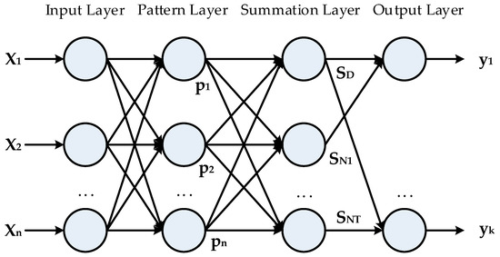
Figure 1.
The structure of the general regression neural network (GRNN).
- (1)
- input layer. The number of neurons is equal to the dimension of the input vector in the learning sample. Each neuron is a simple distribution unit that passes the input variable directly to the pattern layer.
- (2)
- pattern layer. The number of neurons is equal to the number of learning samples. Each neuron corresponds to a different sample, and the neuron transfer function is:where represents the network input variable, is the corresponding learning sample of neuron , and belongs to the width coefficient of the Gaussian function, which is called the smoothing factor.
- (3)
- summation layer. Two types of neurons are used for summation.One kind of calculation formula is , which sums up the output of all neurons in pattern layer, and the connection weight between the pattern layer and each neuron equals 1. The transfer function isAnother calculation formula is , which performs weighted summation on all the neurons in the pattern layer. The connection weight between the th neuron in the pattern layer and the th molecule in the summation layer is the th element of th output sample . The transfer function is
- (4)
- output layer. The number of neurons is equal to the dimension of the output vector in the sample. Each neuron will divide the output of the summation layer, and the output of neuron corresponds to the th element of the estimated result , namelyWhen the smooth factor is very large, is approximately the mean of all the sample-dependent variables. On the contrary, when the smooth factor tends to 0, is very close to the training sample. When the point to be predicted is included in the training sample set, the forecasting value of the dependent variable will be very close to the corresponding dependent variable in the sample. Once encountered, the sample cannot be included in the point, and it is possible to predict a very poor performance, which indicates that the network has a poor generalization ability. When the value of is moderate, the dependent variable of all of the training samples is considered in the estimation , and the dependent variable corresponding to the forecasting point distance is added to the larger weight. Therefore, the value of has a great influence on the forecasting results of the GRNN, and the FOA is used to find the optimal processing of .
2.3. A GRNN Based on the FOA with Parameter Selection
The FOA is a new global optimization method based on foraging behaviors. The fruit flies themselves are superior in smell and vision to other species; specifically, they can collect all kinds of smells in the air and fly in the direction of the food or gather with companions. Thus, there are two steps for searching for food of a fruit fly swarm [30]: (1) use an olfactory organ to collect odors floating in the air and fly towards the food location; and (2) use vision to find food and other fruit flies’ gathering position and fly to that direction. The iterative food searching process of a fruit fly swarm is shown in Figure 2. Compared with PSO, the FOA has strong robustness as a result of the algorithm’s operation not involving multiple loops and complicated functions. An optimization problem with only one parameter can achieve very good results. In this paper, the FOA is utilized to select the best value of the smoothing factor in the GRNN.
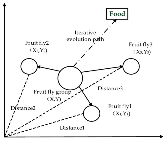
Figure 2.
Iterative food searching process of a fruit fly swarm.
The wind speed forecasting model combining EMD, the FOA, and the GRNN are constructed as illustrated in Figure 3.
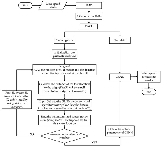
Figure 3.
The flow chart of EMD-FOA-GRNN. EMD: empirical mode decomposition; IMF: intrinsic mode function; PACF: partial autocorrelation coefficient function; FOA: fruit fly optimization algorithm.
The specific steps for wind speed prediction are listed as follows:
Step 1: Decompose the original wind series into a collection of IMFs by EMD. In order to choose a proper input, the partial autocorrelation coefficient function (PACF) is applied to each of the IMFs to select the elements for the training set. For the stationary time series , the so-called k-order lag PACF refers to the correlation between and under the condition of a given middle random variable , or after eliminating the interference of the middle random variable .
Step 2: Initialize the parameters: after many attempts, the optimal population size and the maximum iteration number are respectively proposed as 20 and 50. The initial position of the fruit fly swarm is set as , , where represents the random number generation function. Here, according to general value range of the smoothing factor , the range of random flight distance is set as (–10,10). To avoid overtraining, the samples are divided into two groups to carry out the cross-training.
Step 3: Start searching for the optimum: according to the operation mechanism of the FOA [29], set the number of iterations , and let be the random direction and distance that an individual fruit fly follows to look for food.
Step 4: Evaluate the population: firstly, calculate the distance from the location of the fruit fly to the origin and take the reciprocal of as the smell concentration judgment value .
Secondly, set as the value of the smoothing factor in the GRNN to predict the wind speed. Thirdly, select the root mean square error as the fitness function () to evaluate the disparity between the actual value and forecasting result, and record the corresponding value as the smell concentration . Finally, the fruit fly with the minimal smell concentration can be found out.
Step 5: Record the optimal value. The best smell concentration value , smell concentration judgment , and the and coordinates need to be kept as follows. Then, the fruit flies utilize vision to fly towards that location.
Step 6: Implement iteration optimization. Repeat Step 3 and Step 4 to determine whether the smell concentration is better than the previous one. If it is, go to Step 5 and set .
Step 7: Stop optimization and start prediction. Circulation ends at the maximum number of iterations. Here, the best value of the smoothing factor can be substituted into the GRNN model for wind speed forecasting.
3. Evaluation Criteria of Forecasting Performance
It is the primary issue to determine which forecasting model outperforms the other models, and the performance of the prediction models is usually assessed by statistical criteria: the mean absolute error (MAE), the mean absolute percentage error (MAPE), the root mean square error (RMSE), and the index of agreement (IoA). For the first three indexes, the smaller the values are, the better the forecasting performance is. For the IoA, the closer the value is to 1, the better the forecasting performance is. In addition, an MAPE <10% indicates high prediction accuracy, 10% ≤ MAPE ≤ 20% indicates good prediction, 20% ≤ MAPE ≤ 50% implies acceptable prediction, and an MAPE ≥ 50% implies inaccurate prediction [9]. These four error indexes are defined as follows:
where and are the actual and forecast wind speeds at time period , respectively; is the forecasting period; and represents the mean value of the actual wind speed at time period .
Additionally, in order to show the improvement degree of forecasting errors for different models, is defined as follows:
where and represent the MAE, MAPE, RMSE, and IoA generated by the proposed model and other compared models, respectively.
4. Case Study
4.1. Wind Speed Data
Gansu province, with a wealth of wind energy resources, is one of the top seven 10-million-kilowatt wind power bases heavily invested for construction in China. Located in Jiuquan City, Guazhou is known as “the World Storehouse of Wind Energy”, whose geographical position is shown in Figure 4. In recent years, a series of favorable policies have been issued to promote the further development of wind power generation in this area. The installed wind capacity is expected to reach 6.45 million kW and the annual generating capacity will come to 14 billion kWh in 2015 for the Guazhou region. According to preliminary planning, by 2020, the total installed wind capacity will exceed 10 million kW. Therefore, accurate wind speed forecasting is not only the basis for wind power prediction, but also has profound significance for planning and designing a wind farm, making a schedule for operating the generator, ensuring the safe operation of the electric power system, and improving economic benefits, etc.
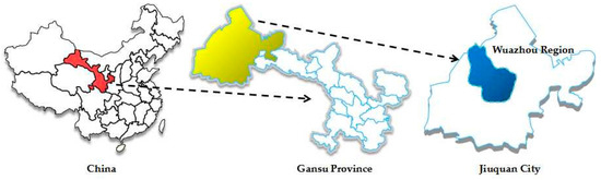
Figure 4.
The geographical location of Guazhou Region.
The wind speed data every 20 min from 28 October 2011 to 1 December 2011 were collected from a wind farm in the northwest of Guazhou, totaling 2520 records. Here, the data from 28 October 2011 to 28 November 2011 are selected as the training set and the remaining 216 data are utilized as the test set. Figure 5 shows the original wind speed time series (including 2304 samplings) with its nonlinear and nonstationary characteristics.
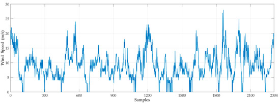
Figure 5.
Original wind speed series from 28 October 2011 to 28 November 2011.
4.2. Forecasting Steps
Step 1: Wind speed decomposition. EMD is applied to decompose the original wind speed series into several IMFs to eliminate the nonstationarity of the data, which may have an impact on prediction accuracy. From Figure 6, it can be observed that until eight independent IMFs and one residue R0 are decomposed, the wind speed time series in this case satisfies the condition of EMD.
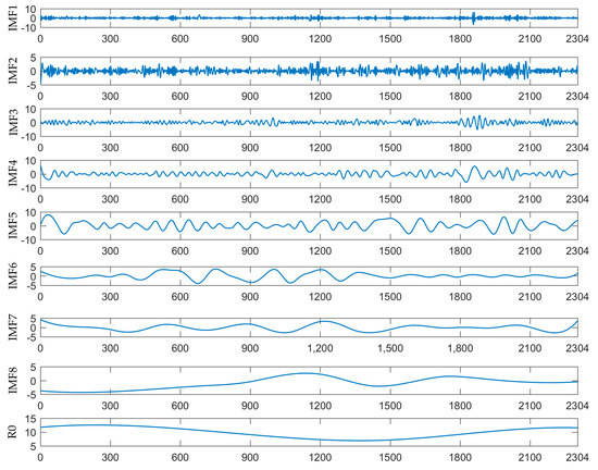
Figure 6.
The EMD results of original wind speed series.
Step 2: Input variables selection based on PACF. Since the weather variables that may affect wind speed cannot be easily collected, and the wind speed shows certain time series characteristics, the wind speed data values before the forecast wind speed point are considered as the input variables of the GRNN, and the PACF is applied to determine the specific input variable number of each of the IMFs and R0. Figure 7 is the plot of the partial correlation analysis of the wind speed, where PACF1~PACF8 stand for IMFs (PACF1~PACF8), respectively, and PACF9 represents the residue (R0). Setting each decomposition wind speed time series as the output variable, if the PACF at lag is out of the 95% confidence interval, is applied as one of the input variables.
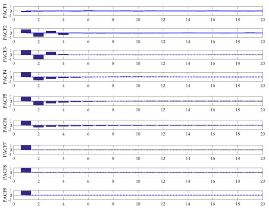
Figure 7.
The PACFs of the IMFs and R0.
So, it is obvious that the input variables of these nine series for the FOA-GRNN are the ones shown as follows.
- IMF1:
- IMF2:
- IMF3:
- IMF4:
- IMF5:
- IMF6:
- IMF7:
- IMF8:
- R0:
Step 3: Wind speed forecasting. The FOA-GRNN is utilized to predict the corresponding sub-series with the selected input variables in Step 2. The final forecasting results for the wind speed from 29 November 2011 to 1 December 2011 are obtained by aggregating the prediction results of each sub-series. The values of the smoothing factor in the GRNN optimized by the FOA are recorded in Table 1 for these IMFs and R0.

Table 1.
The values of the smoothing factor for each FOA-GRNN trained by the IMFs and R0.
Step 4: Comparative analysis of different models. From Figure 8, eight models are presented to predict the wind speed. The ARIMA, BPNN, and GRNN models are three different basic forecasting models. Since PSO and the FOA both belong to the class of swarm intelligent optimization algorithms, there are similarities in the operating mechanism. Thus, the PSO-GRNN and the FOA-GRNN are utilized to test whether the optimization part donates to the prediction accuracy. The EMD-GRNN, the EMD-PSO-GRNN, and the EMD-FOA-GRNN can be applied to explore the effectiveness of EMD. After many attempts, the proper parameters settings in each algorithm are displayed in Table 2. The wind speed actual and forecasting values for different models are shown in Figure 9 and Figure 10.
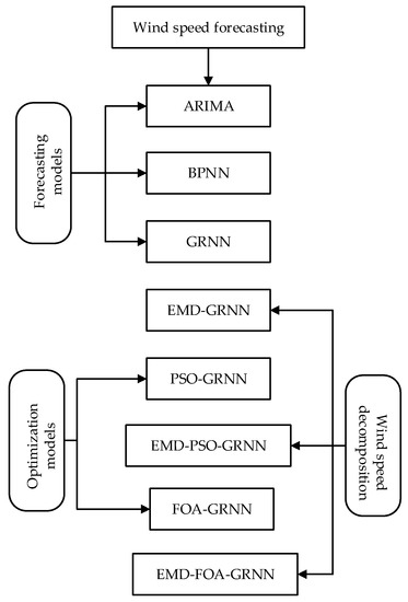
Figure 8.
Comparison framework for wind speed forecasting models. ARIMA: autoregressive integrated moving average.
Table 2.
The parameters settings in each of the comparison models.
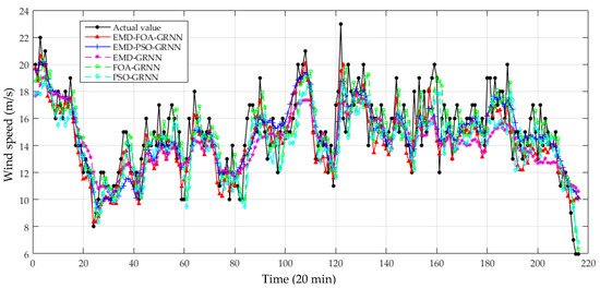
Figure 9.
Prediction results of wind speed from 29 November 2011 to 1 December 2011 (I).
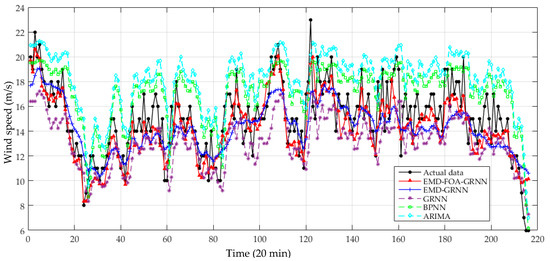
Figure 10.
Prediction results of wind speed from 29 November 2011 to 1 December 2011 (II).
4.3. Results Analysis
Figure 11 displays the degree of correlation between the actual value and predicted values of the wind speed. It can be seen that the forecasted wind speed obtained by the EMD-FOA-GRNN model most correlates to the actual one compared with the FOA-GRNN and EMD-GRNN models.
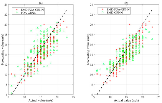
Figure 11.
The correlation between forecasting and actual wind speed. (a) EMD-FOA-GRNN and FOA-GRNN; (b) EMD-FOA-GRNN and EMD-GRNN.
As is presented in Figure 12, the absolute value of error by the EMD-FOA-GRNN model is relatively stable and there are only five error points out of 4 m/s, which means that the forecasting results can be accepted. The accuracy estimation of the predicted wind speed by different models is shown in Table 3. It can be observed that the relative errors in the hybrid models mainly concentrate on the level of less than 10%. Moreover, the number of errors less than 10% generated by the EMD-FOA-GRNN, EMD-PSO-GRNN, and EMD-GRNN models is more than 120, which shows a good performance in wind speed forecasting.
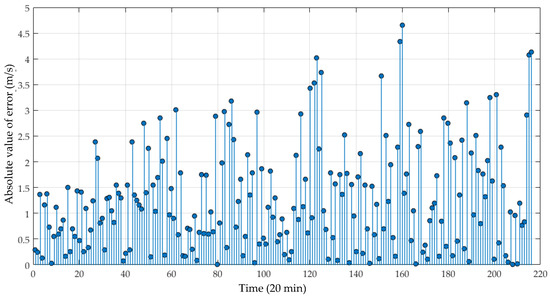
Figure 12.
The absolute value of error by the EMD-FOA-GRNN model.
Table 3.
Accuracy estimation of forecasting models for the test samples.
From Table 4, it can be analyzed that: (a) based on the four evaluation criteria MAE, MAPE, RMSE, and IoA, the proposed model EMD-FOA-GRNN shows the best forecasting performance among the eight models. The MAE, MAPE, RMSE, and IoA of the proposed model is 1.286 m/s, 8.95%, 0.124 m/s, and 0.9070, respectively. (b) by comparing the three single models, the GRNN and the BPNN have higher accuracy than the ARIMA model. Therefore, it can be concluded that intelligent models can obtain better forecasting results than statistical models. Additionally, the GRNN presents more satisfactory performance than the BPNN. The prediction accuracy of the BPNN is closely related to typical training samples and network structure, and it is easy to fall into a local extreme. However, the GRNN, with only one parameter to be optimized, is more suitable for forecasting nonlinear and non-stationary wind speed series. (c) when comparing the EMD-FOA-GRNN with the FOA-GRNN, the EMD-PSO-GRNN with the PSO-GRNN, and the EMD-GRNN with the GRNN, EMD improves the forecasting performance in terms of lower MAE, MAPE, RMSE, and a higher IoA, which proves it can effectively decompose the volatile signals to promote the forecasting capacity. (d) the two optimized models PSO-GRNN and FOA-GRNN produce better results than the single GRNN model. Here, the FOA and the PSO algorithm are utilized to select the appropriate value of the smoothing factor for the GRNN. These two optimization algorithms can effectively enhance the training and learning process so as to avoid falling into a local optimum and improve the global searching ability of the GRNN. Moreover, as seen from these four indexes’ values, the FOA made a better optimal performance than that of PSO, which verified the optimization mechanism of the FOA.
Table 4.
Statistical error measures of prediction methods in Case One.
From Table 5, it can be found that: (a) the forecasting performance of the EMD-GRNN combined with the PSO algorithm and the FOA have been effectively improved. It can be seen that the FOA performs better than the PSO algorithm in improving prediction accuracy, mainly because it is easier to use the FOA to fulfill a global optimization goal with less parameters to be optimized. (b) For the basic EMD-GRNN model, it can be analyzed that the FOA enhances the forecasting accuracy and the MAPE promoted percentage is 18.56%. Similarly, owing to EMD, the promoted percentage of MAPE is 21.35%. (c) The EMD part makes more of a contribution than the FOA part in the EMD-FOA-GRNN model.
Table 5.
Promoted percentage of errors in Case One.
5. Case Two
In order to verify that the proposed model has good adaptability in different times and places, another case which selects the wind speed data in a wind farm located in the middle of Inner Mongolia (shown in Figure 13) is provided in this paper. The study is carried out with the data from 18 February 2012 to 22 March 2012 as the training set and data from 23 March 2012 to 25 March 2012 as the test set. The forecasting results are displayed in Figure 14 and Figure 15. The error analyses are shown in Table 5 and Table 6.
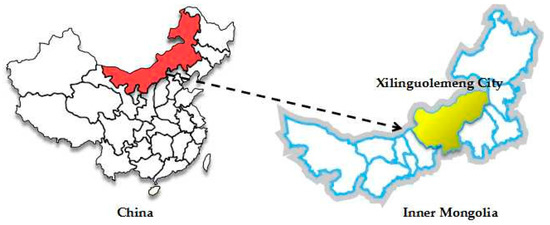
Figure 13.
The geographical location of Xilinguolemeng City.
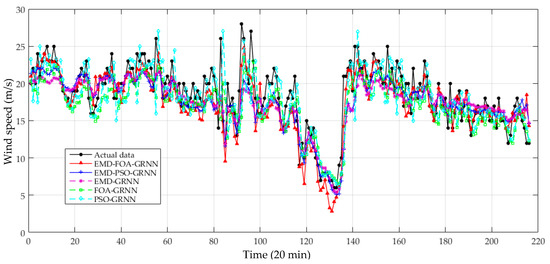
Figure 14.
Prediction results of wind speed from 23 March 2012 to 25 March 2012 (III).
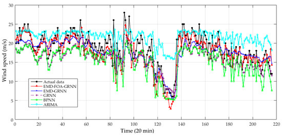
Figure 15.
Prediction results of wind speed from 23 March 2012 to 25 March 2012 (IV).
Table 6.
Statistical error measures of prediction methods in Case Two.
As demonstrated in Table 6 and Table 7: (a) intelligent algorithms have higher accuracy in wind speed forecasting than statistical models. (b) the hybrid models show better performance than the single one. (c) EMD improves the performance compared with the corresponding forecasting models that directly utilize the original wind speed series to make predictions. (d) The EMD-FOA-GRNN presents the best forecasting results among the models, and the EMD part donates much more than the FOA part in improving prediction precision. In all, the results in Case Two once again verify the feasibility and effectiveness of the proposed model.
Table 7.
Promoted percentage of errors in Case Two.
6. Conclusions
This paper presents a hybrid intelligent algorithm for wind speed forecasting. Firstly, EMD is proposed to preprocess the original wind speed signals to eliminate the random fluctuations of the wind speed data. Then, the GRNN model, which is improved by the FOA, is used to forecast the set of IMFs obtained by EMD. The PACF is used to select the arguments of the GRNN and choose the lags of the historical speeds. Major conclusions are summarized as follows: (a) the EMD effectively improves the forecasting performance; (b) the optimization algorithms FOA and PSO increase the strong global searching capability of the model, and the FOA shows better performance; (c) the EMD part contributes more than the FOA in increasing the accuracy of the EMD-FOA-GRNN model; and (d) the error valuation criteria shows that the EMD-FOA-GRNN is a very promising methodology, which can provide a new idea for short-term wind speed forecasting. In addition, with the development of signal processes and intelligent algorithms, there will be more advanced models applied to predict wind speed, which is our study direction in the future.
Supplementary Files
Supplementary File 1Acknowledgments
This work is supported by the Natural Science Foundation of China (Project No. 71471059) and the Fundamental Research Funds for the Central Universities (Project No. 2017XS103). Wei-Chiang Hong thanks the research grant sponsored by the Ministry of Science & Technology, Taiwan (MOST 106-2221-E-161-005-MY2).
Author Contributions
Yi Liang designed this research and wrote this paper; Dongxiao Niu and Wei-Chiang Hong provided professional guidance.
Conflicts of Interest
The authors declare no conflict of interest.
References
- Hu, Q.; Zhang, R.; Zhou, Y. Transfer learning for short-term wind speed prediction with deep neural networks. Renew. Energy 2016, 85, 83–95. [Google Scholar] [CrossRef]
- Wang, J.; Hu, J. A robust combination approach for short-term wind speed forecasting and analysis—Combination of the ARIMA (Autoregressive Integrated Moving Average), ELM (Extreme Learning Machine), SVM (Support Vector Machine) and LSSVM (Least Square SVM) forecasts using a GPR (Gaussian Process Regression) model. Energy 2015, 93, 41–56. [Google Scholar]
- Sawyer, S.; Fried, L.; Shukla, S.; Qiao, L. Global Wind Report 2016—Annual Market Update; Global Wind Energy Council: Brussels, Belgium, 2017. [Google Scholar]
- National Development and Reform Commission. National Climate Change Program (2014–2020); National Development and Reform Commission: Beijing, China, 2014. Available online: http://www.ndrc.gov.cn/zcfb/zcfbtz/201411/W020141104584717807138.pdf (accessed on 30 November 2017).
- Erdem, E.; Shi, J. ARMA based approaches for forecasting the tuple of wind speed and direction. Appl. Energy 2011, 88, 1405–1414. [Google Scholar] [CrossRef]
- Liu, H.; Tian, H.Q.; Li, Y.F. Comparison of two new ARIMA-ANN and ARIMA-kalman hybrid methods for wind speed prediction. Appl. Energy 2012, 98, 415–424. [Google Scholar] [CrossRef]
- Hodge, B.M.; Zeiler, A.; Brooks, D.; Blau, G.; Pekny, J.; Reklatis, G. Improved Wind Power Forecasting with ARIMA Models. Comput. Aided Chem. Eng. 2011, 29, 1789–1793. [Google Scholar]
- Wang, J.; Hu, J.; Ma, K.; Zhang, Y. A self-adaptive hybrid approach for wind speed forecasting. Renew. Energy 2015, 78, 374–385. [Google Scholar] [CrossRef]
- Ramasamy, P.; Chandel, S.S.; Yadav, A.K. Wind speed prediction in the mountainous region of India using an artificial neural network model. Renew. Energy 2015, 80, 338–347. [Google Scholar] [CrossRef]
- Hui, L.; Tian, H.Q.; Li, Y.F.; Zhang, L. Comparison of four Adaboost algorithm based artificial neural networks in wind speed predictions. Energy Convers. Manag. 2015, 92, 67–81. [Google Scholar]
- Zjavka, L. Wind speed forecast correction models using polynomial neural networks. Renew. Energy 2015, 83, 998–1006. [Google Scholar] [CrossRef]
- Babu, C.N.; Reddy, B.E. A moving-average filter based hybrid ARIMA-ANN model for forecasting time series data. Appl. Soft Comput. 2014, 23, 27–38. [Google Scholar] [CrossRef]
- Chen, K.; Yu, J. Short-term wind speed prediction using an unscented Kalman filter based state-space support vector regression approach. Appl. Energy 2014, 113, 690–705. [Google Scholar] [CrossRef]
- Zhou, J.; Jing, S.; Gong, L. Fine tuning support vector machines for short-term wind speed forecasting. Energy Convers. Manag. 2011, 52, 1990–1998. [Google Scholar] [CrossRef]
- Weron, R. Electricity price forecasting: A review of the state-of-the-art with a look into the future. Int. J. Forecast. 2014, 30, 1030–1081. [Google Scholar] [CrossRef]
- Cincotti, S.; Gallo, G.; Ponta, L.; Marco, R. Modeling and forecasting of electricity spot-prices: Computational intelligence vs classical econometrics. AI Commun. 2014, 27, 301–314. [Google Scholar]
- Amjady, N.; Keynia, F. Day ahead price forecasting of electricity markets by a mixed data model and hybrid forecast method. Int. J. Electr. Power Energy Syst. 2008, 30, 533–546. [Google Scholar] [CrossRef]
- Guo, Z.H.; Wu, J.; Lu, H.Y.; Wang, J.Z. A case study on a hybrid wind speed forecasting method using BP neural network. Knowl.-Based Syst. 2011, 24, 1048–1056. [Google Scholar] [CrossRef]
- Liu, H.; Chen, C.; Tian, H.Q.; Li, Y.F. A hybrid model for wind speed prediction using empirical mode decomposition and artificial neural networks. Renew. Energy 2012, 48, 545–556. [Google Scholar] [CrossRef]
- Zhang, W.; Wang, J.; Wang, J.; Zhao, Z.; Tian, M. Short-term wind speed forecasting based on a hybrid model. Appl. Soft Comput. 2013, 13, 3225–3233. [Google Scholar] [CrossRef]
- Liu, D.; Wang, J.; Wang, H. Short-term wind speed forecasting based on spectral clustering and optimized echo state networks. Renew. Energy 2015, 78, 599–608. [Google Scholar] [CrossRef]
- Liu, H.; Tian, H.; Liang, X.; Li, Y. New wind speed forecasting approaches using fast ensemble empirical model decomposition, genetic algorithm, Mind Evolutionary Algorithm and Artificial Neural Networks. Renew. Energy 2015, 83, 1066–1075. [Google Scholar] [CrossRef]
- Liu, H.; Tian, H.Q.; Chen, C.; Li, Y.F. An experimental investigation of two Wavelet-MLP hybrid frameworks for wind speed prediction using GA and PSO optimization. Int. J. Electr. Power Energy Syst. 2013, 52, 161–173. [Google Scholar] [CrossRef]
- Liu, D.; Niu, D.; Wang, H.; Fan, L. Short-term wind speed forecasting using wavelet transform and support vector machines optimized by genetic algorithm. Renew. Energy 2014, 62, 592–597. [Google Scholar] [CrossRef]
- Yu, S.; Ke, W.; Wei, Y.M. A hybrid self-adaptive Particle Swarm Optimization-Genetic Algorithm-Radial Basis Function model for annual electricity demand prediction. Energy Convers. Manag. 2015, 91, 176–185. [Google Scholar] [CrossRef]
- Rahmani, R.; Yusof, R.; Seyedmahmoudian, M.; Mekhilef, S. Hybrid technique of ant colony and particle swarm optimization for short term wind energy forecasting. J. Wind Eng. Ind. Aerodyn. 2013, 123, 163–170. [Google Scholar] [CrossRef]
- Bahrami, S.; Hooshmand, R.A.; Parastegari, M. Short term electric load forecasting by wavelet transform and grey model improved by PSO (particle swarm optimization) algorithm. Energy 2014, 72, 434–442. [Google Scholar] [CrossRef]
- Yeh, W.C.; Yeh, Y.M.; Chang, P.C.; Ke, Y.C.; Chung, V. Forecasting wind power in the Mai Liao Wind Farm based on the multi-layer perceptron artificial neural network model with improved simplified swarm optimization. Int. J. Electr. Power Energy Syst. 2014, 55, 741–748. [Google Scholar] [CrossRef]
- Ren, C.; An, N.; Wang, J.; Li, L.; Hu, B.; Shang, D. Optimal parameters selection for BP neural network based on particle swarm optimization: A case study of wind speed forecasting. Knowl.-Based Syst. 2014, 56, 226–239. [Google Scholar] [CrossRef]
- Pan, W.T. A new fruit fly optimization algorithm: Taking the financial distress model as an example. Knowl.-Based Syst. 2012, 26, 69–74. [Google Scholar] [CrossRef]
- Li, H.Z.; Guo, S.; Li, C.J.; Sun, J.Q. A hybrid annual power load forecasting model based on generalized regression neural network with fruit fly optimization algorithm. Knowl.-Based Syst. 2013, 37, 378–387. [Google Scholar] [CrossRef]
- Yuan, X.; Liu, Y.; Xiang, Y.; Ye, X. Parameter identification of BIPT system using chaotic-enhanced fruit fly optimization algorithm. Appl. Math. Comput. 2015, 268, 1267–1281. [Google Scholar] [CrossRef]
- Dai, H.; Liu, A.; Lu, J.; Dai, S.; Wu, X.; Sun, Y. Optimization about the layout of IMUs in large ship based on fruit fly optimization algorithm. Opt. Int. J. Light Electron Opt. 2015, 126, 490–493. [Google Scholar] [CrossRef]
- Wang, Y.H.; Yeh, C.H.; Young, H.W.V.; Hu, K.; Lo, M.T. On the computational complexity of the empirical mode decomposition algorithm. Phys. Stat. Mech. Appl. 2014, 400, 159–167. [Google Scholar] [CrossRef]
- Samet, H.; Marzbani, F. Quantizing the deterministic nonlinearity in wind speed time series. Renew. Sustain. Energy Rev. 2014, 39, 1143–1154. [Google Scholar] [CrossRef]
- Hong, Y.Y.; Yu, T.H.; Liu, C.Y. Hour-Ahead Wind Speed and Power Forecasting Using Empirical Mode Decomposition. Energies 2013, 6, 6137–6152. [Google Scholar] [CrossRef]
- Wang, J.; Zhang, W.; Li, Y.; Wang, J.; Dang, Z. Forecasting wind speed using empirical mode decomposition and Elman neural network. Appl. Soft Comput. 2014, 23, 452–459. [Google Scholar] [CrossRef]
- Huang, N.E. The empirical mode decomposition and the Hilbert spectrum for nonlinear and non-stationary time series analysis. R. Soc. Lond. Proc. 1998, 454, 903–995. [Google Scholar] [CrossRef]
- Specht, D.F. A general regression neural network. IEEE Trans. Neural Netw. 1991, 2, 568–576. [Google Scholar] [CrossRef] [PubMed]
© 2017 by the authors. Licensee MDPI, Basel, Switzerland. This article is an open access article distributed under the terms and conditions of the Creative Commons Attribution (CC BY) license (http://creativecommons.org/licenses/by/4.0/).