Asynchronous Fault Location in Transmission Lines Considering Accurate Variation of the Ground-Mode Traveling Wave Velocity

Abstract

This paper proposes a grounding fault location method in transmission lines based on time difference of arrival (TDOA) of ground-mode and aerial-mode traveling waves (TWs). The frequency-dependent characteristics of transmission lines cause different frequencies to have different attenuations and phase lags of different frequency components in traveling waves, which leads to the change of TWs velocities with different propagation distances. Due to these different propagation paths, the wave velocity variations of ground-mode should be considered as a main variable while the velocity of aerial-mode can be seen as a constant factor. A quadratic function that can illustrate the tendency of variation of ground-mode wave velocity is proposed by considering the relation between the wave velocity and fault distance. The least squares method is used to solve the quadratic function of different lines. Combining the quadratic formula and the incident TWs of each mode detected at both terminals of the line, a novel fault location method is proposed. First, according to the maximum and minimum ground-mode velocities, a fault scope can be acquired. Then, more accurate fault scopes and ground-mode velocities can be obtained by iteration computation. Finally, an accurate fault position is acquired when the fault scope is sufficiently small. PSCAD/EMTDC software is used to conduct fault simulations in order to verify the feasibility and accuracy of the method.

1. Introduction

In many countries, the energy base is far from the power load center so long transmission lines are necessary for power transmission. These transmission lines are hundreds of kilometers in length and can be damaged by severe weather and human activities. The traditional fault location is based on the line protection action. Numerous methods have been proposed for transmission line protection [1], with no consideration of the exact fault location, causing the need for time-consuming line patrols. It is necessary to find the exact fault location in transmission lines. Locations of faults on overhead power lines for the repair purposes is still a subject of great interest to researchers and utilities personnel, which dates back to the eighties [2,3].

Currently, there are mainly two kinds of fault location methods: (a) steady-state method and (b) transient-state methods [4]. The steady-state methods do not need high sampling frequency and can be realized by existing measurements [5]. However, these methods is susceptible to line parameters, fault resistances, load swing, etc. Steady-state methods are not suitable for long transmission lines with many changeable factors such as line transposition, load swing, etc. [6,7,8]. The transient-state methods are more stable with respect to these factors and have a better accuracy and robustness. In [9], a current frequency component based method for cable fault location was proposed. It was verified by PSCAD/EMTDC that the method had high accuracy and strong robustness. However, it needs a higher sampling frequency [10,11,12,13,14,15]. For long transmission lines which are of great importance to power companies, transient-state methods have been widely used for their reliability.

Within the category of transient-state method, representative traveling wave-based methods can be further divided into two different types: single-ended and double-ended methods [16]. On the one hand, single-ended methods only need data from one terminal of the line, which is independent from the synchronization and communication equipment [17]. The difficulties of these methods lie in identifying the TWs reflected wave from a fault location. However, the reflected wave is often disturbed by the waves reflected or refracted from other line terminals. In [18], a wavelet transform is employed in order to construct the traveling wave propagation waveform. By comparing the constructed and real recorded waveforms, the reflection wave of the fault point can be identified. Lin proposed a single-ended fault location method based on the time-frequency characteristics of traveling waves [19]. This method is used for calculation of the zero-mode velocity and identification of the reflected wave font. How to ensure the computational accuracy of the Lipschitz exponent is a challenging question. On the other hand, the double-ended method needs data from double terminals and synchronization [20,21]. In [20], Global Positioning System (GPS) is utilized to obtain synchronized transient voltage measurements from all of the receiving ends. A traveling wave based fault location algorithm is presented for hybrid multi-terminal transmission systems which consists of one onshore overhead line and multiple offshore submarine cables. Similarly, GPS and Artificial Neural Network approaches are used to synchronize voltage and current signals at both ends of the transmission line [21].

Based on the above TW methods, more improved asynchronous fault location methods have been proposed [22,23,24,25,26], which are independent from the effect of wave velocities. Most of these methods are in the time domain. The time stamp of transient traveling wave arrival is critical, which is related to the velocity of the transient traveling wave. Attenuation should be considered due to the fact that the TWs on long transmission lines are changeable and related to the characteristics of the traveling wave, especially when the ground-mode TWs are used. In [22], the time stamps of different modes, arrived at measuring points are utilized. According to the fault location formula and based on a time difference of different modes at both ends, this method eliminates the influence of traveling wave velocity from the formula and does not need synchronization. However, the authors ignored that the velocities of ground-mode TWs have various values depending on the fault position. Due to the traveling wave characteristics, when a fault is not in the middle of a transmission line, the velocities of ground-mode at both sides of the fault point are different, which cannot be eliminated. The fault location error is directly proportional to the distance between the fault point and the middle of line. This is a easily neglected problem. Reference [23] gives a method for identifying the reflected wave from a fault point, which is based on the fault position estimation proposed by [26]. The communication system latency is considered to create a fault area to make sure the time stamp of the reflected wave from the fault point can be correctly identified. The time synchronization system between two terminals is necessary for auxiliary pre-estimations of a fault location. Reference [24] analyses the traveling wave propagation characteristic with a distributed parameter model. To tackle the key problem of ground-mode velocity estimation, an iterative method based on prior knowledge is proposed. However, there are deviations when the ground-mode velocities are calculated by the center pseudo-frequency of wavelet transform. In [25], the author considered the dispersion effect of traveling wave and proposed a compensation method for a better fault location result but the synchronization is still required.

As analyzed above, there are few fault location methods that thoroughly considers the traveling wave characteristics, which play important roles in the fault location detection, especially when the ground-mode traveling wave is used. The ground-mode velocity is vital for accurate fault location in long transmission lines where the attenuation is severe. To address this problem, this paper first analyzes the characteristics of traveling waves. Then, to analyze the velocity of the ground-mode, which changes severely with different fault distances, a formula is proposed based on theoretical analysis and experimental results. Combing the derived formula with the fault location method, a novel fault location method has been proposed to determine an actual ground-mode velocity. Considering the fact that the traveling wave measuring device are available and the synchronization technology is not available in some lines, the proposed method uses a double-ended transient voltage traveling wave without synchronization and identifies the second traveling wave head. Finally, PSCAD/EMTDC simulations have been carried out under different fault conditions to verify the reliability and accuracy of the proposed method.

2. Analysis of the Traveling Wave Characteristics

2.1. Frequency-Dependent Characteristics of Traveling Wave

Current and voltage propagating in transmission lines are in the forms of electromagnetic waves. The wave equations are generally given as below:

$$\begin{array}{l}\frac{d^{2}U}{\partial x^2}=ZYU\\ \frac{d^{2}I}{\partial x^2}=YZI\end{array}$$

(1)

U and I are the phasor voltage and current values in frequency domain. Z and Y are the series impedance and parallel admittance matrix of the transmission line, respectively:

$$\begin{array}{l}Z=R+j\omega L\\ Y=G+j\omega C\end{array}$$

(2)

R, L, G, C are the resistance, inductance, conduction and capacitance of transmission line, respectively. The Karrenbauer transform [27] shown in Equation (3) is used to transform the coupled three phases to independent modes 0, 1, 2 where the mode 0 is the ground-mode and the modes of 1 and 2 are the aerial-modes in engineering [9]. The transform is applicable for the current and voltage traveling waves.

$$\left[\begin{array}{c}{U}_0\\ U_1\\ U_2\end{array}\right]=\frac{1}{3}\times \left[\begin{array}{ccc}1& 1& 1\\ 1& -1& 0\\ 1& 0& -1\end{array}\right]\left[\begin{array}{c}{U}_A\\ U_B\\ U_C\end{array}\right]$$

(3)

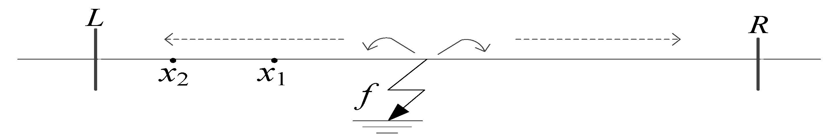
when a fault occurs in a transmission line, just like an equivalent reverse voltage step pulse applied at the fault point, which is equal to the pre-fault phase voltage. The step pulse is a band-width signal, including a broad frequency band from Hz to MHz. Thus, the transient traveling waves of the current and voltage are produced and propagated to both sides of the line as shown in Figure 1.

Equation (1) shows the propagation of traveling waves in the frequency domain, which can be transformed into the time domain as in Equation (4). The traveling waves of the current and voltage signals have the similar expressions.

$$I(x,t)=\sqrt{2}{I}^{+}{e}^{-\alpha (\omega )x}\cos (\omega t-\beta (\omega )x+{\varphi }_{+})+\sqrt{2}{I}^{-}{e}^{\alpha (\omega )x}\cos (\omega t+\beta (\omega )x+{\varphi }_{-})$$

(4)

where α(ω) is the attenuation factors and β(ω) is the phase distortion factors of line. The propagation coefficient of line is defined as $\gamma =\alpha +j\beta$.

Equation (4) shows that a traveling wave consists of a forward wave and a backward wave. The traveling wave attenuates exponentially with distance. The propagation coefficient plays an important role in the propagation of the traveling wave.

For any line, the propagation coefficient of each mode is decided by the line parameters. As shown in Equation (5), m = 0 is the ground-mode and m = 1, 2 is the aerial-mode.

$${\gamma }_m={\alpha }_m(\omega )+j{\beta }_m(\omega )=\sqrt{Z_m{Y}_m}=\sqrt{(R_m(\omega )+j\omega L_m(\omega ))(G_m(\omega )+j\omega C_m(\omega ))}$$

(5)

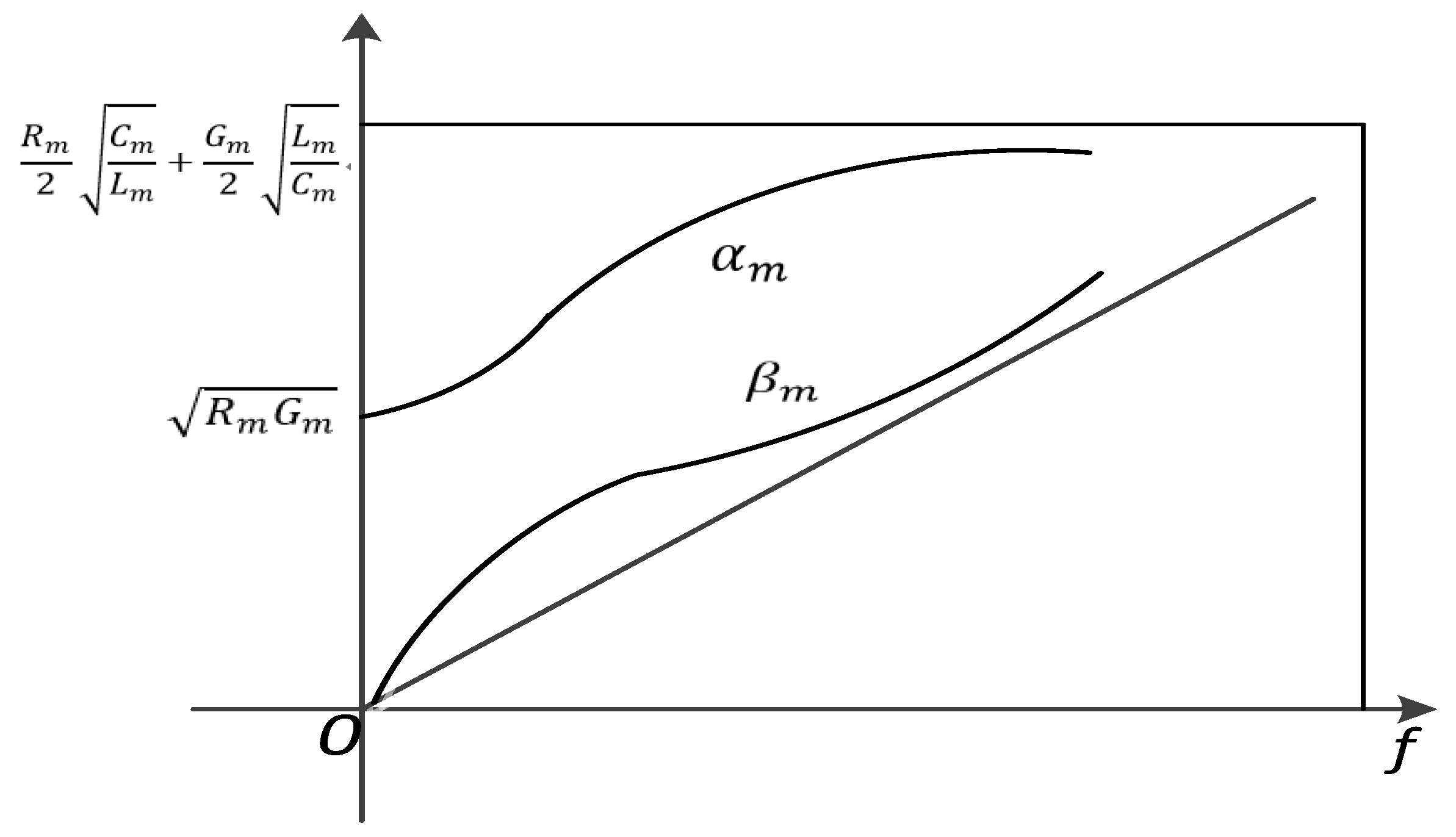
The terms R_m(ω), L_m(ω), G_m(ω) and C_m(ω) are the resistance, inductance, conductance and capacitance of transmission lines, respectively. Considering the frequency dependent characteristic of the lines, these parameters are the frequency-dependent. Among them, the R_m($\omega$) and L_m(ω) change more obviously with frequency comparing to G_m(ω) and C_m(ω). The ${\alpha }_m$ and ${\beta }_m$ in frequency domain are expressed in Equations (6) and (7).

According to Equations (6) and (7), Figure 2 gives the characteristics of curves ${\alpha }_m(\omega )$, ${\beta }_m(\omega )$ in frequency. For ${\alpha }_m(\omega )$, it is in proportion to the frequency. Due to the different propagation path, ${\alpha }_0(\omega )$ is greater than ${\alpha }_1(\omega )$, ${\alpha }_2(\omega )$. The reason is that the impendence of earth is higher than the lines. The attenuation factor of aerial-mode is relatively small and changeless, and that of ground-mode is great and frequency-dependent in comparison:

$${\alpha }_m(\omega )=\sqrt{\frac{1}{2}[R_m(\omega )G_m-{\omega }^2{L}_m(\omega )G_m+\sqrt{(R^2{}_m(\omega )+{\omega }^2{L}^2{}_m(\omega ))(G^2{}_m+{\omega }^2{C}^2{}_m)}]}$$

(6)

$${\beta }_m(\omega )=\sqrt{\frac{1}{2}[{\omega }^2{L}_m(\omega )C_m-R_m(\omega )G_m+\sqrt{(R^2{}_m(\omega )+{\omega }^2{L}^2{}_m(\omega ))(G^2{}_m+{\omega }^2{C}^2{}_m)}]}$$

(7)

Ignoring the attenuation factors, the traveling waves propagate along in the transmission lines with a certain speed, which is:

$$v=\frac{\omega }{\beta (\omega )}$$

(8)

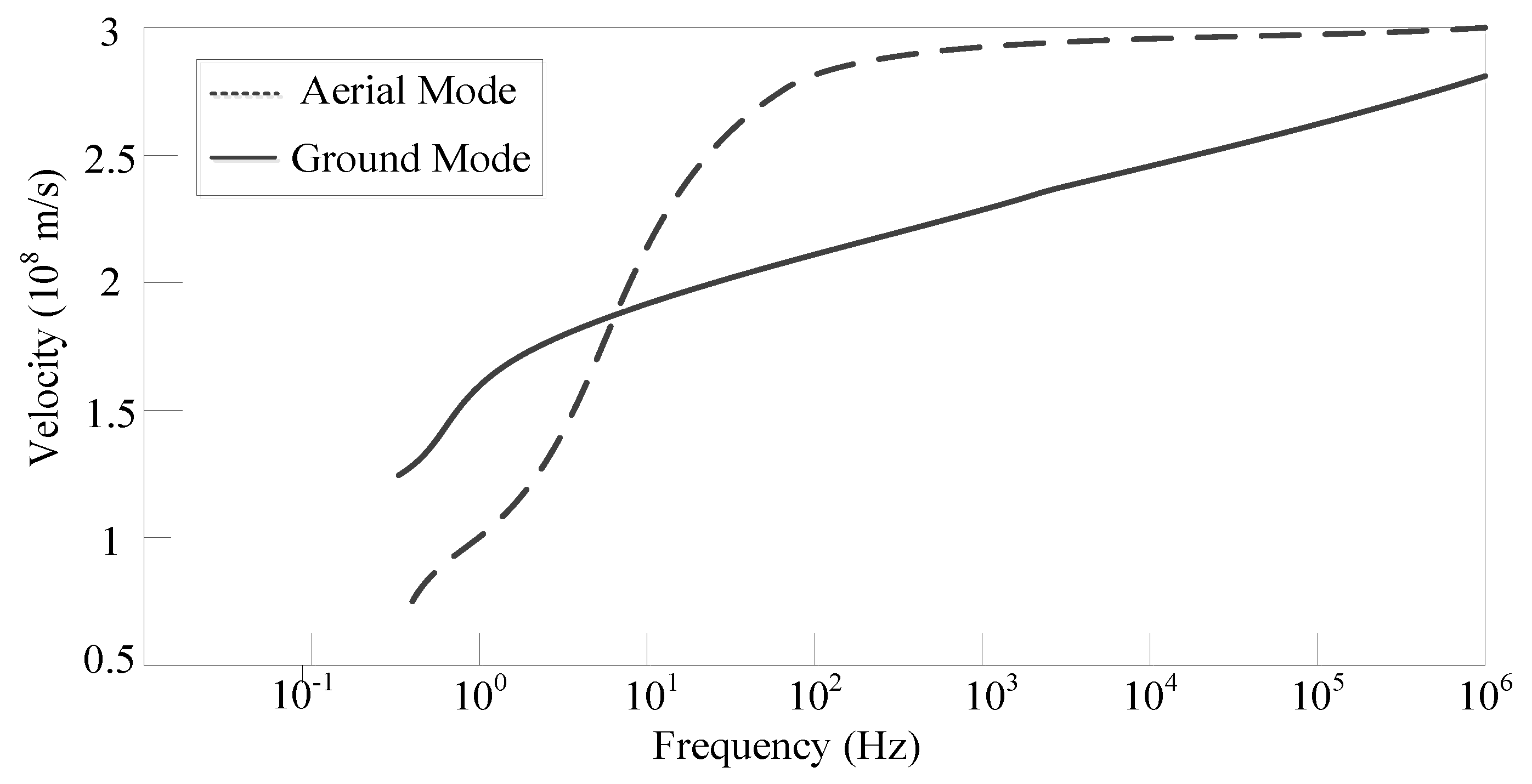
According to the Equations (7) and (8), the relationship curve of velocities and frequencies is shown in Figure 3 which indicates that the ground-mode velocity is approximately linear with respect to frequency and the aerial-mode velocity is constant at high frequency (above 1 kHz). Different frequency signals have different speeds for ground-mode traveling waves. The measuring velocity of traveling wave depends on the highest frequency signal which can be detected.

As analyzed above, the velocity of traveling wave is vital for many fault location algorithms. When a fault occurs, the transient TWs contain high frequency signals. If there are no attenuation factors, the velocity of traveling wave is equal to the speed of the light. As signals with different frequencies have different attenuation factors and velocities, some high frequency signals are immeasurable at measuring points and the measuring velocity of a fault-traveling wave is uncertain within different fault distances.

2.2. The Change of Traveling Wave Velocity with Fault Distance

Equation (8) gives the expression of velocity that does not take the attenuation factor into account. The attenuation factor plays an important role in measuring velocities at measuring points. Equation (4) illustrates that the amplitude of traveling wave attenuates exponentially. The amplitude of first detected transient traveling wave head can be seen as the amplitude superimposition of the highest frequency signals in one sampling interval:

$$A={\displaystyle {\sum }_i{e}^{-x{\alpha }_i}{f}_i(t)}$$

(9)

where f_i(t) is the amplitude of the component in traveling waves with frequency i and A is the detected amplitude of traveling wave head at a measuring point.

As shown in Figure 1, supposing the amplitude of measured traveling wave at x₁ is A₁, the amplitude of measured traveling wave at x₂ is A₂ and sampling time is ∆t. The highest frequency signal components combined with A₁ have the strongest attenuation when travelling toward x₂. As a result, some of those frequencies are attenuated severely and the traveling wave fault location equipment cannot be triggered. Then, the measured signals of x₂ are composed of subsequent lower frequency signals. The dominant frequency of x₂ is lower than that of x₁. According to Figure 3, the velocity of traveling wave at x₂ is smaller than that of x₁. The initial traveling wave is a pulse signal with continuous frequency spectrum. The attenuations of the traveling wave in different frequencies have exponential decay characteristics and the velocity is approximately linear with respect to the frequency. The variation tendency of traveling wave velocity affected by fault distance can be described as a monotonic function.

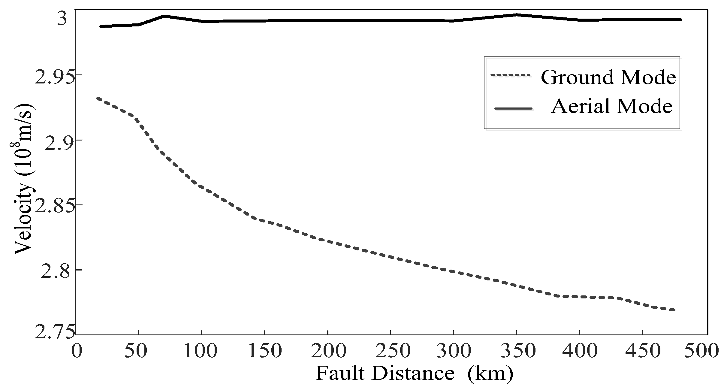
Based on Figure 1, the LGJ-240/30 line has been used for verifying the assumption. The length of the line is 500 km. Figure 4 shows the tendency of ground-mode velocity and aerial-mode velocity.

The attenuation factors are different with the different propagation paths. The ground-mode traveling wave has relatively higher factors of decay. The change of ground-mode velocity is more dramatic than that of the aerial-mode. Without loss of generality, the velocity of ground-mode can be seen as a constant factor which is changed slightly in a finite length line. The ground-mode velocity shows an obviously monotonic descent with the increase of the fault distance. It is inappropriate to take the ground-mode velocity as a known quantity with the unknown fault distance. A monotonic function of ground-mode velocity can benefit the fault location results.

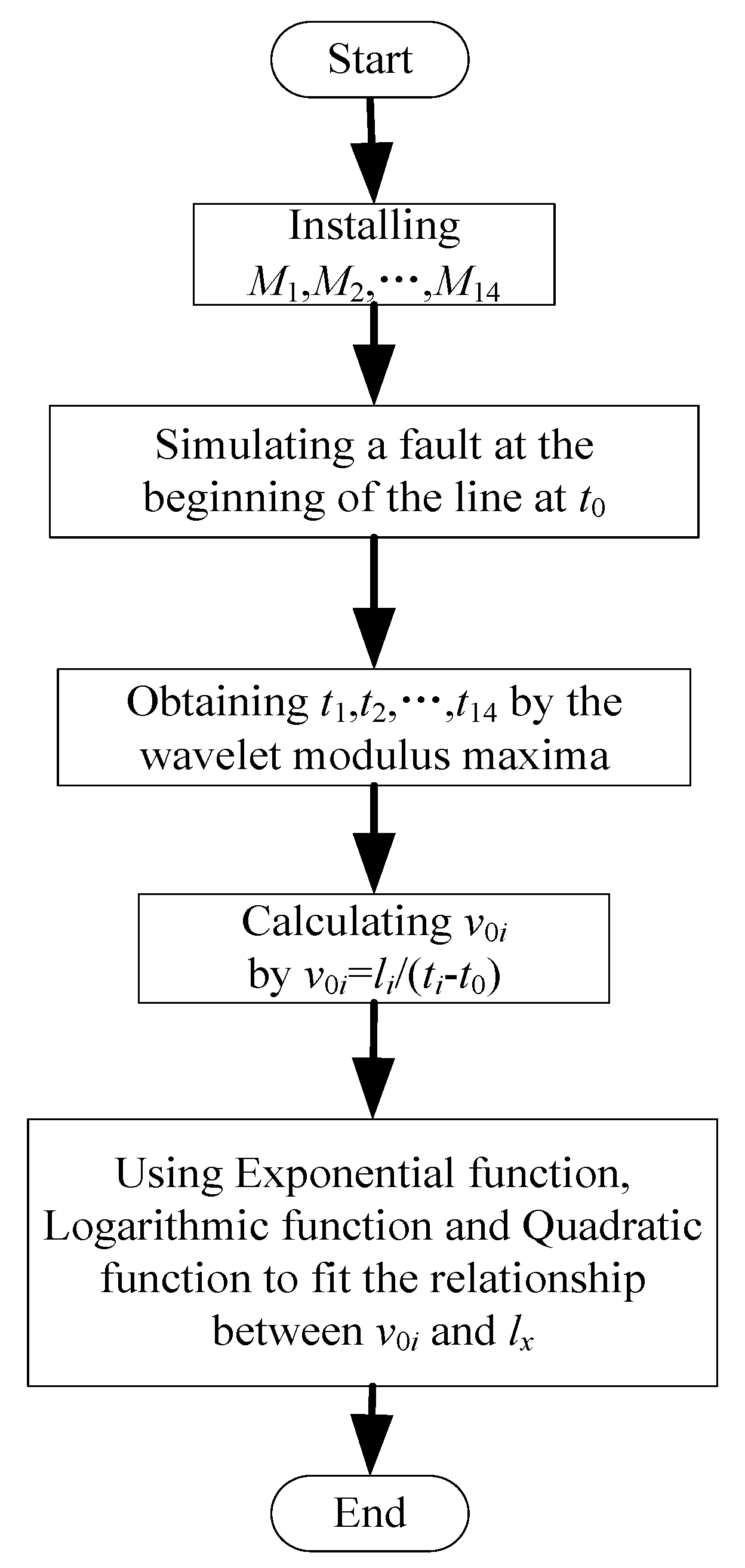
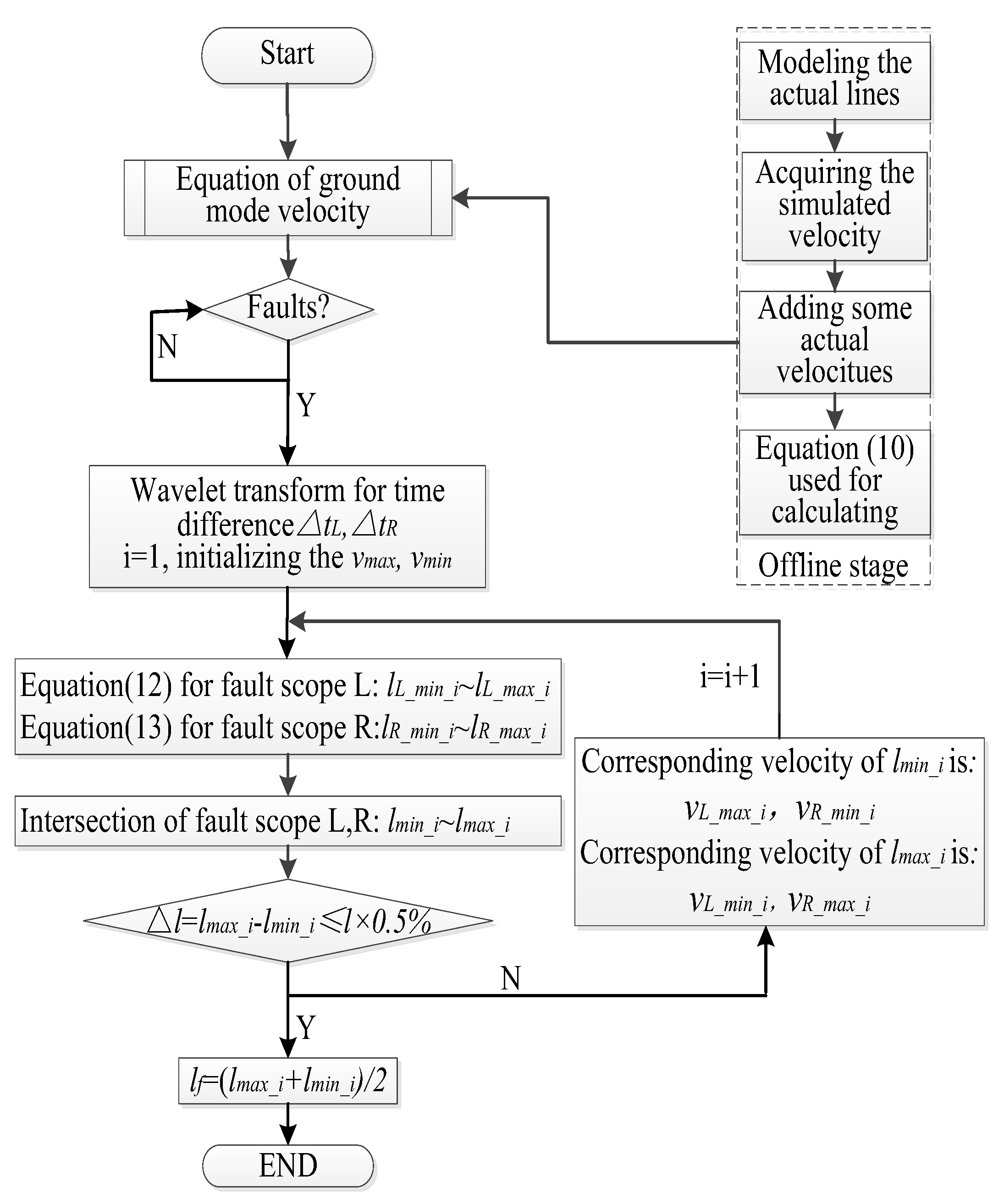
In order to fit the relationship between the ground-mode wave velocity and fault distance, fault simulations and calculations are carried out in the following steps: (1) 14 measurement points denoted as M₁, M₂, …, M₁₄ are installed along the line with the distances l₁, l₂, …, l₁₄ from the local terminal respectively; (2) a fault is simulated at the local terminal of the line at t₀; (3) the ground-mode traveling wave signal acquired at each measurement point is analyzed by wavelet transform and the corresponding arrival time stamp t_i is extracted based on wavelet modulus maximum; (4) the ground-mode velocity of each location where the measurement point is mounted can be calculated according to the following equation:

$$v_{0i}=\frac{l_i}{t_i-t_0}(i=,2,\dots ,14)$$

(10)

(5) The exponential function, logarithmic function and quadratic function are used to fit the relationship between v₀ and l_x. The flowchart of the above steps are illustrated in Figure 5.

From the above steps, it should be noted that it is of great essence to determine the arrival time stamps by wavelet transform, the details of which are shown as follows:

First, the initial traveling wave signal to be analyzed was imported in Matlab Wavelet Tookit. Next, the signal was decomposed into four levels by a Daubechies 6 wavelet. Then, the detailed and approximate coefficients were exported. Finally, the modulus maximum value of detailed coefficients of d1 level was calculated to identify the arrival time stamp of the traveling wave.

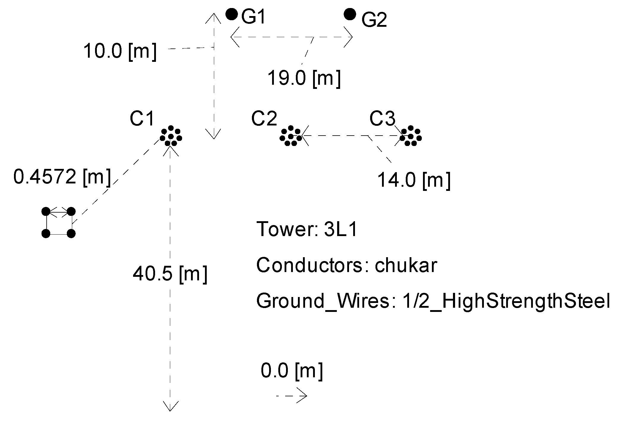
The numerical results of Figure 6 are shown in the following

Table 1. The Numerical results of ground-mode velocity for fitting.

Velocity v0 (105 km/s)	Fault Distance lx (km)	Velocity v0 (105 km/s)	Fault Distance lx (km)
2.950	10	2.817	200
2.928	20	2.805	250
2.914	50	2.794	300
2.888	70	2.784	350
2.861	100	2.771	400
2.847	150	2.770	450
2.828	170	2.762	480

. Three-phase current signals can be transformed into aerial-mode and ground-mode by Karrenbauer transform shown in Equation (3). The arrival time of ground-mode current traveling wave is computed based on Wavelet transform modulus maximum. At last, the ground-mode velocity can be calculated by Equation (10).

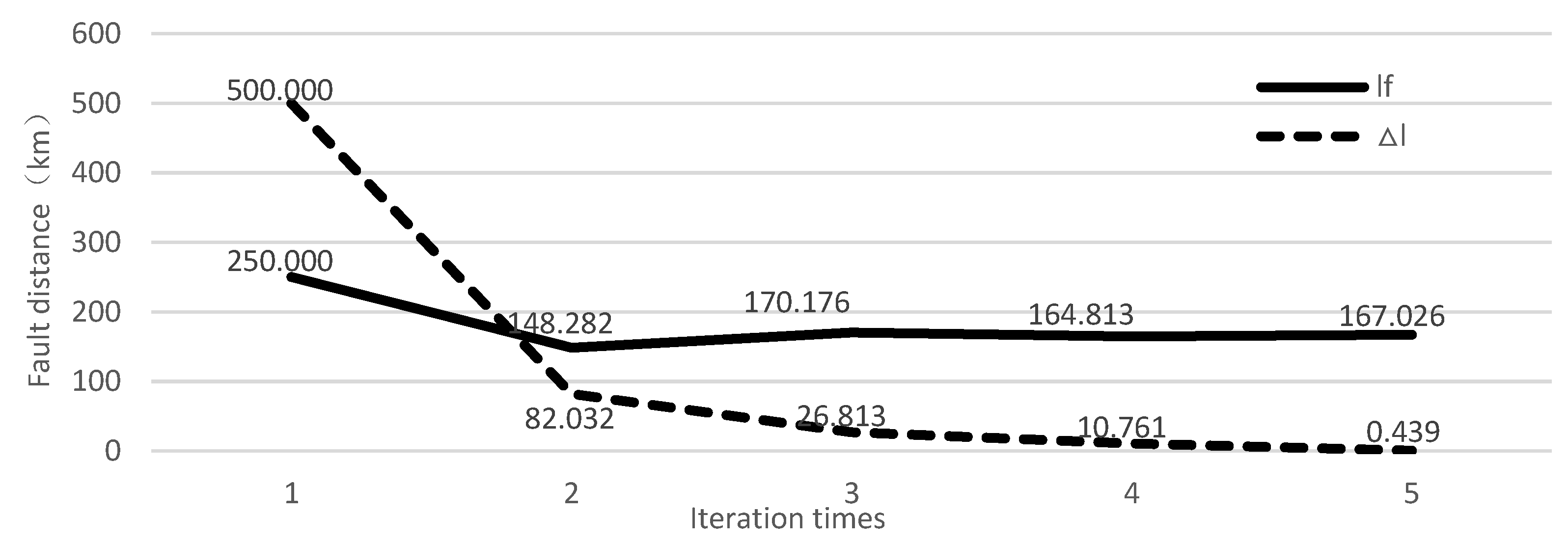
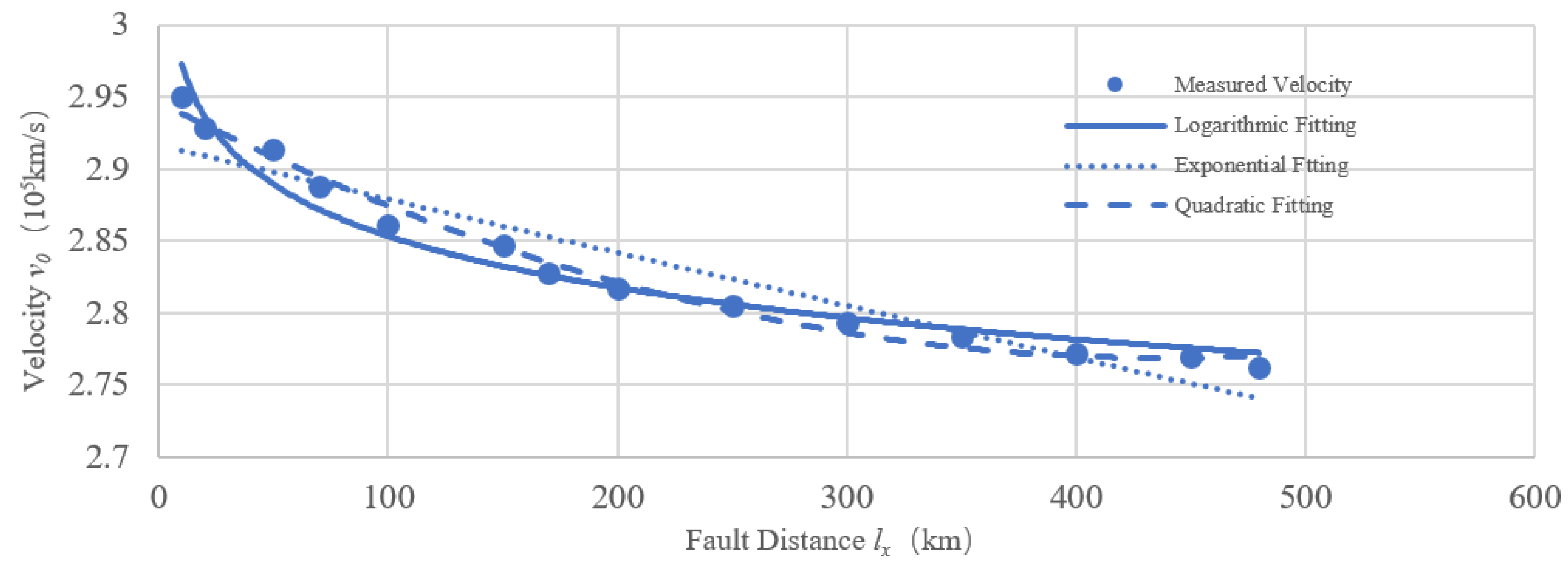
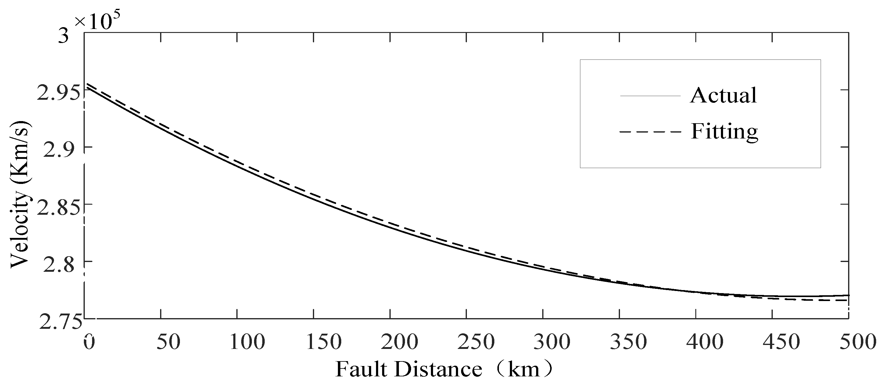
As previously analyzed, the initial traveling wave with sufficiently high frequencies has higher attenuation factor, which causes a stronger change of velocity than that from a further distance. The trend of measured velocity is that the closer to the fault point the faster the changes. Therefore, an exponential function, logarithmic function and quadratic polynomial function with the above tendency have been used for the velocity fitting. The result is shown in Figure 5. The fitting functions and the goodness of fit (R²) are:

• Exponential function: $v_0=28.7\times e^{-0.0047x}$, $R^2=0.883$;
• Logarithmic function: $v_0=-0.037\ln (x)+2.98$, $R^2=0.9622$;
• Quadratic function: $v_0=1\times {10}^{-6}\cdot x^2-9\times {10}^{-4}\cdot x+2.956$, $R^2=0.9783$;

Using this method, MATLAB (MathWorks, Natick, MA, USA) program fits different lines with different lengths. The goodness of fit R² is given in

Table 2. The R² of different lines with different length.

Line Types	LGJ-240/30			LGJ-500/45			LGJ-800/70
Length (km)	Goodness of Fit (${\mathit{R}}^{\mathbf{2}}$)
	Exponential	Logarithm	Quadratic	Exponential	Logarithm	Quadratic	Exponential	Logarithm	Quadratic
300	0.898	0.945	0.971	0.952	0.923	0.986	0.922	0.966	0.987
500	0.883	0.962	0.978	0.941	0.952	0.99	0.91	0.975	0.983
700	0.908	0.957	0.983	0.887	0.943	0.977	0.892	0.948	0.969
1000	0.947	0.961	0.986	0.854	0.901	0.988	0.906	0.921	0.992

.

From Table 2, we can see that each selected function can fit the tendency of the ground-mode velocity. However, the quadratic function fits better than the others and performs better in calculating the velocity along the transmission lines. Thus, the quadratic function is used for describing the relation between the ground-mode velocity and the fault distance.

Based on the above analysis, for any transmission line, the general quadratic function about the ground-mode velocity and the fault distance is defined as below:

$$v_0=A\cdot x^2+B\cdot x+C$$

(11)

A, B, C are the unknown coefficients determined by the lines; x is the fault distance from measured points; v₀ is the corresponding ground-mode velocity.

Acquiring the quadratic function by MATLAB fitting, it is necessary to have significant fault data and information, collected along the lines, which is impossible for operating lines. The least squares method [28] can be used, which only needs more than three points. Therefore, some ground-mode velocities can be found based on the simulation model in PSCAD/EMTDC (Manitoba HVDC Research Centre, Winnipeg, Canada) and using the actual parameters of line. However, the error between the simulation and actual lines is inevitable. In order to correct the error, few velocities achieved by the circuit breakers can be used for the least square method. The breakers commonly have a certain distance between each other, which the fitting correction of tendency can benefit from:

$$\left[\begin{array}{c}A\\ B\\ C\end{array}\right]=C^{-1}{X}^{T}v$$

(12)

Among them, $C=X^{T}X$, $X=\left[\begin{array}{ccc}{x}_1^2& x_1& 1\\ x_3^2& x_2& 1\\ \dots & \dots & \dots \\ x_n^2& x_n& 1\end{array}\right]$, $v=\left[\begin{array}{c}{v}_0^1\\ v_0^2\\ \dots \\ v_0^n\end{array}\right]$.

3. Fault Location Method

3.1. Fault Location Based on the Time Difference of Modes

Figure 7 depicts a time-space diagram for a line monitored at two terminal lines, where t_L0, t_L1, t_R0, t_R1 are the arrival time stamps of incident earth and aerial-mode TWs at buses L and R; v₁ is the aerial-mode TW propagation velocity, which doesn’t change along the line; v_L0 and v_R0 are the ground-mode TW propagation velocities at two-terminal measurements respectively; x is the fault distance and l is the line length.

For the terminal L:

$$\{\begin{array}{c}x=(t_{L1}-t_0)\cdot v_1\\ x=(t_{L0}-t_0)\cdot v_0\end{array}$$

(13)

Eliminating the initial fault time, t₀:

$$x=\frac{\Delta t_L{v}_1{v}_{L0}}{v_1-v_{L0}}$$

(14)

For the terminal R:

$$l-x=\frac{\Delta t_R{v}_1{v}_{R0}}{v_1-v_{R0}}$$

(15)

Among them: $\Delta t_L=t_{L0}-t_{L1}$, $\Delta t_R=t_{R0}-t_{R1}$.

The accurate time-tap of transient traveling wave head arrived at the measurement is important for the fault location algorithm. In long High Voltage Transmission Lines, a typical method is to use a secondary signal of a current transformer (CT) to detect the wave front of the transient TWs. The detection of the current traveling waves needs TWs detecting devices in each line of a substation, which complicates the fault location system and has higher hardware requirements. The voltage traveling wave method only needs to measure the voltage in the bus. Coupling capacitor voltage transformers (CCVT) is a measuring transforming that is widely used in transmission line for voltage measurement and can be used for the extraction of transient signals. In reference [29], it is pointed out that CCVT may have several resonant models and the frequency response may present obvious bandstop and bandpass characteristics due to the stray capacitances in CCVT. To this problem, some substations have additional sensors set up to measure transient voltage traveling waves and some improved CCVTs with good high-frequency response for traveling wave are used [30]. In the proposed method, the arrival time-stamp of transient traveling wave head can be obtained by detecting the singularity and abrupt change point in the signal. Reference [31] proves that the CCVT has a good performance in transforming the singularity and abrupt change point in the voltage signal.

According to [32,33,34], the performance of wavelet transform is great in capturing the transient wave-head. Thus, the Daubechies 6 (db6) wavelet is used to compose the transient wave-head into four levels. The arrival time of modulus maximum detail coefficients at the first level (d1) is used as calibration time. The frequency band of d1 corresponds to 250 kHz–500 kHz at the 1 MHz sampling frequency. The frequency band of d1 is the highest frequency TWs which decides the propagation velocity of transient TWs.

In Equations (14) and (15), the propagation velocities of ground-mode $v_{L0}$ and $v_{R0}$ are uncertain with different fault distances. Considering the quadratic function about the relation between ground-mode velocity and fault distance, a more accurate fault location algorithm can be obtained.

3.2. Proposed Method

The proposed method estimates the accurate fault location by iteratively calculating the actual ground-mode velocity according to the fitted relationship. The method can be divided into two stages: off-line ground-mode velocity fitting and on-line fault location. The core ideas of the proposed method are described below and Figure 8 shows the iteration procedure of the method.

The ground-mode velocity in a transmission line changes within a certain range. In other words, if the velocity measured is denoted as $v_{\max }$ and $v_{\min }$ with a fault occurring at the local and remote terminals respectively, the measuring velocities at both terminals should stay in the range ($v_{\min }$,$v_{\max }$) wherever the fault occurs on the other locations of the line. In this paper, the relationship between the ground-mode velocity and fault distance is fitted off-line by the general quadratic function shown in Section 2.2. Therefore, $v_{\max }$ and $v_{\min }$ can be determined directly by setting the fault distance to be 0 and l in the fitted curve.

When a fault is detected in the transmission line, the following on-line fault location steps are conducted. First, the time difference $\Delta t_L$ and $\Delta t_R$ at the local and remote terminals can be computed by applying a wavelet transform to the ground-mode and aerial-mode traveling waves acquired at the two terminals. Next, substituting $v_{\min }$ and $v_{\max }$ into Equations (18) and (19) with the time difference $\Delta t_L$ and $\Delta t_R$, four fault distances l_{L_min}, l_{L_max}, l_{R_min} and l_{R_max} are obtained and two fault ranges ($l_{L\_\min \_1},l_{L\_\max \_1}$) and ($l_{R\_\min \_1},l_{R\_\max \_1}$) can be determined. The intersection of the two fault ranges is taken as the fault range ($l_{\min \_1},l_{\max \_1}$) for the first iteration, which lie within range of the line as analyzed in Section 3.3. Then, according to the fitted relationship between ground-mode velocity and fault distance, the ground-mode velocities $v_{L\_\min \_1}$, $v_{L\_\max \_1}$ and $v_{R\_\min \_1}$, $v_{R\_\max \_1}$ corresponding to $l_{\min \_1}$ and $l_{\max \_1}$ can be determined. Last, the steps mentioned above are repeated until the stopping criterion defined in Equation (16) is satisfied and the final fault location P_f after n time iterations is computed using Equation (17):

$$\Delta l=l_{\max \_n}-l_{\min \_n}$$

(16)

$$P_f=\frac{(l_{\min \_n}+l_{\max \_n})}{2}$$

(17)

The fault location process is shown in Figure 8.

3.3. Convergence of Proposed Method

In order to achieve the fault points, the convergence of proposed method should be guaranteed. Figure 9 is the iteration diagram.

As shown in the analysis, the ground-mode velocity is decreasing with the increase in fault distance. After iterating n times, the fault range is $(l_{\min \_n},l_{\max \_n})$. The velocities for n + 1 are $v_{\min \_n}$, $v_{\max \_n}$. The iteration fault scope of n + 1 is:

$$l_{\min \_n+1}=\frac{(t_{L0}-t_{L1})v_1{v}_{\min \_n}}{v_1-v_{\min \_n}}=\frac{(t_{L0}-t_{L1})v_1}{\frac{v_1}{v_{\min \_n}}-1}$$

(18)

$$l_{\max \_n+1}=\frac{(t_{L0}-t_{L1})v_1{v}_{\max \_n}}{v_1-v_{\max \_n}}=\frac{(t_{L0}-t_{L1})v_1}{\frac{v_1}{v_{\max \_n}}-1}$$

(19)

According to Equations (18) and (19), if the smaller ground-mode velocity v_{min_n} is substituted in Equation (18), a smaller calculated fault distance than actual fault distance could be obtained. Otherwise, a larger calculated fault distance could be acquired. Four fault distances l_{L_min}, l_{L_max}, l_{R_min} and l_{R_max} could be computed by substituting the arrival time differences ∆t_L and ∆t_R between ground-mode and aerial-mode travelling waves detected at both terminals of the line. The minimum distance scope composed by l_{L_min}, l_{L_max}, l_{R_min} and l_{R_max} could be selected for calculating the new ground-mode velocities v_{min_n+1} and v_{max_n+1}. Repeating the above steps would result in the converged fault distance P_f. To clarify the process of iteration, a numerical example (a fault 167 km away from the local terminal) is displayed in

Table 3. Iteration result of the fault location at 167 km.

Iteration Times	vR_min	vR_max	vL_min	vL_max	L	R	R-L < 0.5% × L
1	2.7698	2.954	2.7698	2.954	107.266	189.298	no
2	2.7735	2.7896	2.8343	2.8787	156.770	183.583	no
3	2.7818	2.7881	2.8370	2.8505	159.433	170.194	no
4	2.7824	2.7848	2.8436	2.8492	166.807	167.246	yes

below.

When only one-end of data is used, such as L, the situation of $l_{L\_\max }>l$ may occur when the fault is near the terminal R. In this situation, the $l_{R\_\min }$ calculated by the data of terminal R is on the line. As shown in Figure 10, the intersection of l_scope is always on the transmission line and the velocities for the next iteration always exist.

4. Simulation and Test Results

4.1. The Model of Simulation

PSCAD/EMTDC software is used to construct a 500 kV AC transmission system model as Figure 7. The length of the transmission lines is 500 km. The sampling rate is 1 MHz and the 16 bits A/D resolution is used. The type of lines is 4 × LGJ-400/35 and earth resistively is 150 $\mathsf{\Omega }\cdot \mathrm{m}$. Figure 11 shows the model of the towers.

4.2. Example Analysis

4.2.1. The Quadratic Function of Ground-Mode Velocity

According to the model, some velocities along the transmission line are simulated. Benefiting from the reclosing devices, few actual ground-mode velocities can be obtained, which will modify the results. Using Equation (12), the quadratic function of this line is:

$$v_0=8.49\times {10}^{-7}\cdot x^2-7.93\times {10}^{-4}\cdot x+2.954$$

(20)

Figure 12 compares the actual ground-mode velocity curve and the calculated velocity curve. It can be seen that the proposed fitting method has a great performance and the maximum error is less than 0.2%, which meets the demand of engineering application. For this transmission line, the maximum ground-mode velocity is $v_{\max }=2.954\times {10}^5$ km/s and the minimum ground-mode velocity is $v_{\min }=2.796\times {10}^5$ km/s. The aerial-mode velocity is a constant value of $2.994\times {10}^5$ km/s.

4.2.2. Validation of Proposed Fault Location Method

A single-phase ground fault is set at the distance of 167 km from terminal L. The wavelet transform is used to capture the arrival time of each mode. Figure 13 shows the time differences of ground-mode and aerial-mode at each end. An appropriate adjustment is adopted on TWs amplitude for easily observation and analysis, which does not affect the time difference of aerial-mode and ground-mode. The time differences at L, R are $\Delta t_L=29$ μs, $\Delta t_R=84$ μs separately. Figure 14 gives the results of each iteration.

Figure 14 shows that the proposed method has quick convergence and high accuracy. After iterating five times, the calculated fault scope is 166.806 km–167.245 km and $\Delta l=0.439$ km, $500\times 0.5\%\Delta t_R$ when the iteration process is over. The fault location is 167.026 km from terminal L, which only deviates slightly from the actual situation. Though the iteration is used, the complexity of proposed method is low. The process of fault location can be accomplished instantaneously.

4.3. Fault Location Results

The Equation (21) is used to calculate the relative error:

$$d\%=\frac{\left|l_{x\_mea}-l_{x\_real}\right|}{l}\cdot 100\%$$

(21)

where $l_{x\_real}$ is the actual fault distance, $l_{x\_mea}$ is the distance of location result and the l is the length of the transmission line.

Table 4. The influence of fitting error on the fault location results.

Fault Distance (km)	69	172	268	339	420	479
Fitted velocity(×108 m/s)	2.9032	2.8427	2.8025	2.7828	2.7707	2.769
Actual velocity(×108 m/s)	2.9018	2.8429	2.8024	2.7836	2.7723	2.7668
Relative error of velocity (%)	0.05	0.01	0.00	0.03	0.06	0.08
Fault location(km)	69.18	172.12	268.05	339.09	420.14	179.21
Relative error of location (%)	0.036	0.024	0.01	0.018	0.028	0.042

shows effect of fitting error of velocities on the fault location results. From Figure 12, the tendency of fitted ground-mode velocity conforms to the actual situation, which ensures the convergence of the proposed method. Although there are errors between the fitted and actual velocities, the small errors cannot change the tendency. For a fault, the fitted velocities around fault point play an important role in the accuracy of fault location. The fitting error in other places will not affect the fault location result. The fitted ground velocity fully satisfies the requirements of engineering applications, so the proposed method has a great robustness.

In order to verify the adaptability of the proposed method, different faults have been simulated.

Table 5. The fault location results by 0.1 Ω fault resistance.

Fault Distance/km	Fault Angle/($°$)	Fault Location/km
		Proposed
10	30	9.88
	90	9.92
250	30	250.05
	90	250.01
485	30	484.89
	90	485.07

and

Table 6. The fault location results by 90° by fault angle.

Fault Distance/km	Fault Resistance/($\Omega$)	Fault Location/km
		Proposed
10	0.1	9.92
	300	10.37
250	0.1	250.01
	300	250.21
485	0.1	485.07
	300	485.33

show the influences of fault resistance and fault angle on the fault location method. From Table 5 and Table 6, it can be concluded that the fault location error is increasing with the rise of fault resistance when the fault inception angle keeps constant. On the other hand, when the fault resistance remains constant, the fault location error is minimum with a 90° fault inception angle. Under different fault conditions, the maximum error and minimum error of the accurate fault location using this method are 0.37 km and 0.01 km, which well meets the requirement of practical engineering application.

In order to show the advantages of the proposed method, we compare in

Table 7. A comparison with the state-of-the-art fault location methods.

Year	Method	Min Error (km)	Max Error (km)	Synchronization
2012	[19]	0.16	2.52	no
2015	[21]	0.02	14.32	yes
2017	[23]	0.031	0.067	no
2017	Proposed method	0.01	0.37	no

several methods published in recent years with the presented method.

The results reveal that: (1) the proposed method has great performance no matter where the faults occur along the transmission line. The absolute error is less than 0.37 km and the relative error is less than 0.2%, which meets the requirement of practical applications; (2) with respect to the traditional synchronized method in [21], the proposed method has better accuracy and does not need synchronization. Due to the effect of different angles and fault resistances on the voltage amplitude of the initial transient TWs, the fault location results fluctuate slightly but do not affect the accuracy of the measurement; (3) compared with the single-ended method [19], the proposed method is fast and has much less computation time and can be completed quickly when a fault occurs. Due to the attention of TWs, the computational accuracy of Lipschitz exponent is decreased with the increase of the fault distance which affects the fault location. The positioning accuracy of proposed method is independent from the fault distance; (4) comparing with the method given in [21], the proposed method has a great fault location result performance, which illustrates that the change of ground-mode velocity is important in fault location when the ground-mode TWs are used. As the attenuation factors cannot be ignored, the proposed quadratic function can describe the change tendency of ground-mode velocity with fault distance, which improve the accuracy of fault location greatly; (5) although the method described in reference [23] is asynchronous, the second reflected wave front must be detected, which brings difficulty to accurate fault location since it is usually hard to detect the second reflected wave front. However, the presented method only utilizes the arrival time stamps of the first wave fronts of the modulus traveling waves which are easily detected. In addition, the presented method does not require synchronization, it is independent of line parameters, and has high fault location accuracy.

5. Conclusions

The inaccuracy of the ground-mode velocity is an important issue for fault location detection based on the ground-mode TWs. To address this problem, this paper thoroughly investigated the relation between fault distance and ground-mode velocity. The measured velocity is based on the phase distortion factors and frequency while it is also affected by the attenuation factors. Based on the fundamental cause of the ground-mode velocity change, the general trend of the velocity change can be obtained. Comprehensive simulations have been carried out and the quadratic function performed very well in describing the change of ground-mode velocity. The change tendency of velocity can benefit the fault location algorithm using the ground-mode velocity.

The proposed fault location method neither need synchronization nor identification of a second wave font, which is a cost-effective. The fault location results are slightly affected by the fault phase and resistance. The accuracy of the fault location can be as high as the synchronized two-ended TWs fault location method with strict time synchronization.

Nowadays, traveling wave fault location devices are widely installed on HV transmission lines, which is convenient for applying the proposed fault location method.