Reliable Biomass Supply Chain Design under Feedstock Seasonality and Probabilistic Facility Disruptions

Abstract

While biomass has been recognized as an important renewable energy source which has a range of positive impacts on the economy, environment, and society, the existence of feedstock seasonality and risk of service disruptions at collection facilities potentially compromises the efficiency and reliability of the energy supply system. In this paper, we consider reliable supply chain design for biomass collection against feedstock seasonality and time-varying disruption risks. We optimize facility location, inventory, biomass quantity, and shipment decisions in a multi-period planning horizon setting. A real-world case in Hubei, China is studied to offer managerial insights. Our computational results show that: (1) the disruption risk significantly affects both the optimal facility locations and the supply chain cost; (2) no matter how the failure probability changes, setting backup facilities can significantly decrease the total cost; and (3) the feedstock seasonality does not affect locations of the collection facilities, but it affects the allocations of collection facilities and brings higher inventory cost for the biomass supply chain.

1. Introduction

To ensure future energy security and sustainability, renewable energy has attracted considerable attention from researchers in both academia and industry. Biomass is one of the renewable energy sources upon which policy makers rely to reduce greenhouse gas emissions. The biomass resource base is composed of a wide variety of forestry and agricultural materials, industrial-process residues, and municipal-solid and urban-wood residues [1]. Its appeal is due to its potential worldwide availability, reasonable conversion efficiency, and ability to be produced and consumed on a CO₂-neutral basis. However, renewable energy production from biomass faces many challenges due to uncertainty in its feedstock supply and reliability in its supply chains [2,3].

Unlike general commodities, agricultural biomass is usually characterized by seasonal availability, thus dictating the need of storing large amounts of biomass for lengthy time periods, which in turn leads to high inventory holding costs for supporting the year-round operation of a biorefinery [4]. Moreover, weather related variability and competing uses of waste biomass in a dynamically changing market have strong impacts on the uncertainty of feedstock supply. Zhou, et al. [5] investigated the availability of straw, one of the most important biomass resources in China. They pointed out that the amount of straw harvested in September and October is over 50% of that in the whole year while nearly no straw can be collected during January to April. The variations in feedstock yields can alter the delivery decisions and may consequently affect the setting of the supply chain. Therefore, the impact of feedstock seasonality on the integrated biomass supply chain design should be fully addressed. In addition, variations in feedstock supply motivate the use of collection facilities that serve as temporary storage warehouses. In periods of high supply, biomass can be stored in these facilities and wait for downstream demand. However, collection facilities may be disrupted from time to time due to reasons such as natural disasters, power outages, accidents, market competition, or labor actions [6]. These kinds of risks can cause severe damage to supply chain efficiency and service quality. Once a collection facility fails, the affected biorefineries will be forced to use other functioning facilities, by overcoming longer distances, to collect feedstock from the farmers, or give up collection and incur a penalty. Either way, supply chain cost increases. The adverse effect may be further exacerbated if multiple collection facilities fail simultaneously. Therefore, reliable network design considering disruption risk becomes an important issue in optimization of supply chains.

In this paper, we aim at designing a reliable supply chain for biomass against seasonal variation of feedstock and the probabilistic disruptions of the collection facility. We formulate a multi-period model in which both available feedstock and disruption risk vary seasonally. The proposed model includes location decisions, inventory decisions, sourcing decisions (from farmers), as well as biomass shipment quantity decisions over a specific planning horizon. The objective function is to minimize the total cost of the biomass supply chain, including transportation cost, fixed facility cost, and inventory holding cost. Both disruption risks and seasonality issues are captured by a set of chance-constraints. Computational results are provided to offer managerial insights based on a real-world case in Hubei, China. The main contributions of our paper are as follows:

• We propose a three-stage multi-period model for the design of biomass supply chain under feedstock seasonality and probabilistic facility disruptions. The output of our model provides biomass shipment quantity, inventories, locations, and allocations of collection facilities.
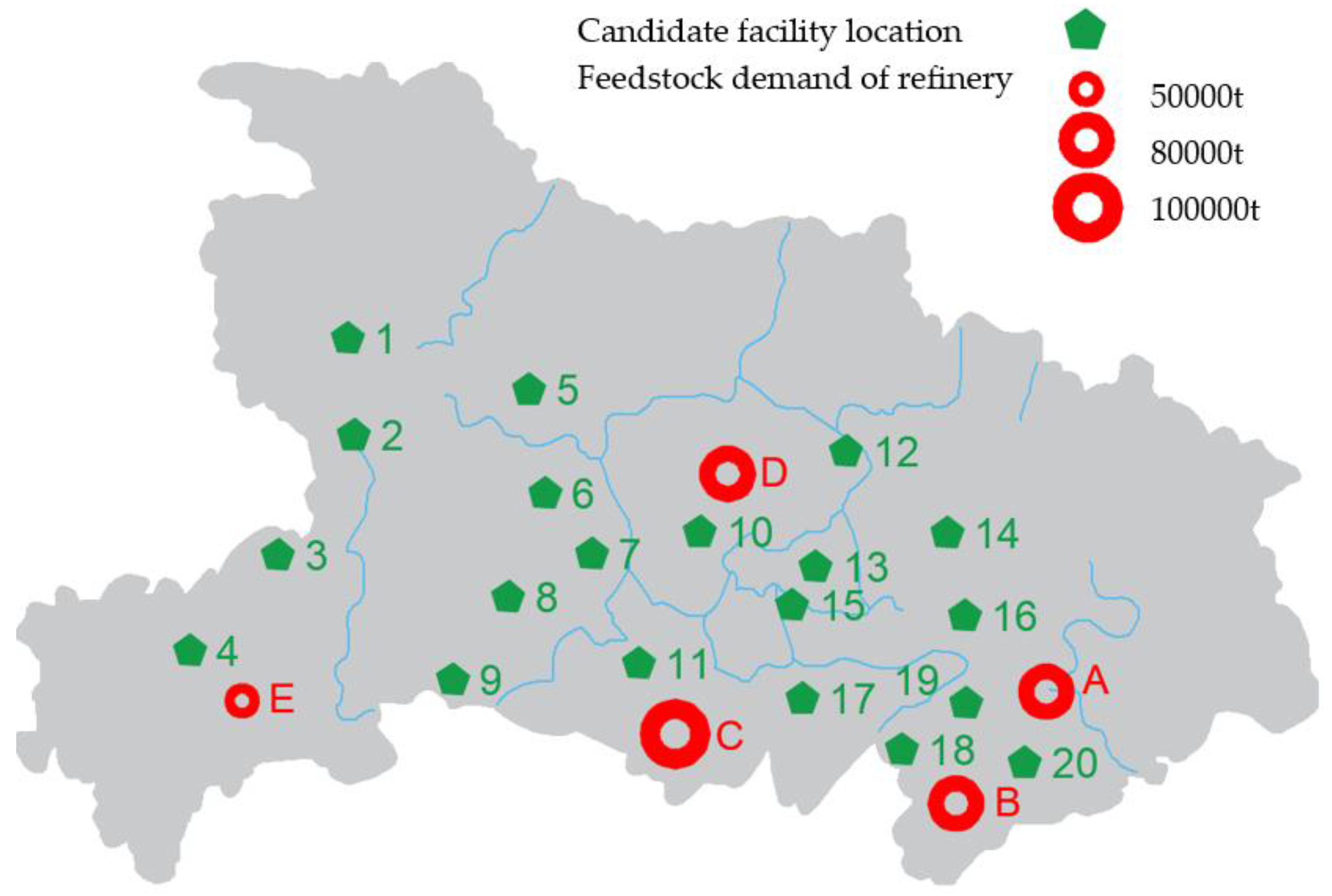
• Through case studies, we explore the relationship between biomass supply chain decisions (e.g., collection facility locations and inventories) and uncertainties (e.g., disruption risks and feedstock seasonality). The results provide valuable guidance and managerial insights for the Hubei NE Biofuel Company, the biggest biofuel company in Hubei Province, China.

The rest of this paper is organized as follows. We review the related literature in Section 2. Then, we develop a mathematical model for the reliable biomass supply chain design with facility disruptions and feedstock seasonality. The methods and data are introduced in Section 3. In Section 4, we provide the results of the case study and conduct numerical experiments to quantify the impacts of feedstock seasonality and failure probability on the optimal supply chain configuration and the total cost. Finally, conclusions and some directions for future research are discussed in Section 5.

2. Literature Review

2.1. Biomass Supply Chain Design

In recent years, a lot of researchers have focused on the design of biomass supply chain. Rentizelas, et al. [7] analyzed three most frequently used biomass storage methods and applied them to a case study. They introduced a multi-biomass supply chain design aiming at reducing the storage space requirement. Ekşioğlu, et al. [8] proposed a mathematical model to determine the amount of biomass shipped and processed as well as the number, size and location of biorefineries under the biomass seasonality. Chen and Fan [9] established a two-stage stochastic programming model to support strategic planning of bioenergy supply chains. The feedstock resource allocation was optimized in an uncertain environment. Xie, et al. [10] developed a multistage, mixed-integer programming model that fully integrated multimodal transportation options into a cellulosic biofuel supply chain under feedstock seasonality. Huang, et al. [11] focused on the design of an efficient biofuel supply chain system against seasonal variations and uncertainties of feedstock supply. Pettersson, et al. [12] proposed a geographically explicit optimization model to investigate the future production of next-generation biofuels from forest biomass in Sweden. Ouraich and Lundmark [13] developed a geographically-explicit model of price determination of forest biomass for Sweden. They constructed regional supply curves and investigated the impacts on equilibrium prices of increased demand for forest biomass. Nasiri, et al. [14] proposed a whole life asset supply chain optimization model aimed at identifying the optimal energy generation capacities and the optimal levels of biomass ordering and storage with time-varying feedstock.

Most of the studies on design of biomass supply chains have considered a single planning time period. Only a few studies have considered multi-period optimization of biomass supply chains. Huang, et al. [15] developed a multistage model that integrated spatial and temporal dimensions for strategic planning of future bioethanol supply chain systems. A dynamic, spatially explicit, and multi-echelon mixed integer linear programming modeling framework was presented by Dal-Mas, et al. [16]. You and Wang [17] considered diverse conversion pathways and feedstock seasonality. Walther, et al. [18] presented a multi-period mixed integer programming model for integrated location, capacity, and technology planning. Akgul, et al. [19] presented a multi-objective, static modelling framework for the optimization of hybrid first/second generation biofuel supply chains. A novel multi-period mixed-integer programming model capable of taking into consideration biomass quality, seasonality, and weather related supply restrictions was developed by Gautam, et al. [20]. Marufuzzaman and Ekşioğlu [21] managed congestion in the biomass supply chain via dynamic freight routing, and the proposed system used multi-modal facilities in different time periods of a year to hedge against biomass seasonality.

2.2. Disruption Risks in Supply Chain

Uncertainty and risks have been shown to play a crucial role in supply chain design. Following the definition by Tang [22], supply chain risks are categorized into operational risks and disruption risks. The operational risk refers to those recurrent risks such as supply and demand uncertainties that are inherent in supply chains. A disruption risk usually refers to external disruptions caused by natural and man-made disasters [23]. The papers reviewed in the preceding subsection generally address operational risks. In this subsection, we discuss papers that have addressed disruption risks.

Supply chain facilities are susceptible to disruption risks due to various failures, such as man-made failures, natural disasters, transportation delay, and power outages [24,25,26]. A lot of researchers have focused on the supply chain reliability and resilience against disruption risks. Snyder and Daskin [27] introduced the reliability fixed charge location problem and the reliability p-median problem. Both models used a bi-objective formulation in which one objective corresponds to the “normal” cost (ignoring disruptions) and the other corresponds to the expected “failure” cost. Berman, et al. [28] generalized the classical p-median problem on a network to explicitly include the probabilistic disruptions, and analyze structural and algorithmic aspects of the resulting model. Cui, et al. [29] proposed a compact mixed-integer program formulation and a continuum approximation model to study the reliable uncapacitated fixed charge location problem. Lim, et al. [30] considered a facility location problem incorporating two types of facilities, one is unreliable and another is reliable. The reliable facility is not subject to disruption, but is more expensive than the unreliable facility. Li and Ouyang [6] studied the reliable uncapacitated fixed charge location problem where facilities were subject to spatially correlated disruptions. Shen, et al. [31] studied a reliable facility location problem. They formulated this problem as a two-stage stochastic program and then as a nonlinear integer program. Chen, et al. [32] considered a reliable joint inventory-location problem. The facility locations, customer allocations, and inventory management decisions were optimized when facilities were subject to disruption risks. Lim, et al. [33] considered a facility location problem in the presence of random facility disruptions. They assumed that facilities can be protected with additional investments. The output of the model showed that the impact of misestimating the correlation degree was much less significant relative to that of misestimating the disruption probability. Xie, et al. [34] considered an integer programming formulation of a reliable location-routing problem in which facilities are subject to the risk of probabilistic disruptions. Facility locations, delivery routing and backup plans were optimized to minimize facility setup, routing, and customer penalty costs. Hasani and Khosrojerdi [35] proposed six resilience strategies to mitigate the risk of correlated disruptions and developed an efficient parallel Taguchi-based memetic algorithm. Khosrojerdi, et al. [36] presented a robust optimization approach for a mixed integer nonlinear programming model while random disruptions happen in a power supply chain network. Zhao, et al. [37] studied an integrated supply chain system problem that simultaneously determines facility location, multi-modal transportation configuration, and inventory management decisions under both facility disruption risks and operational uncertainties.

Traditional biomass supply chain studies always assume that a collection facility will remain functioning throughout its life cycle. However, like many other facilities, biomass collection facilities are exposed to disruptions risks such as water scarcity, flooding, routine maintenance, or adverse weather condition [25]. Once facility disruption happens, excessive operational cost may occur due to the reallocation of biomass supply to more distant facilities [38]. Therefore, considering the disruption risks of collection facility, reliable supply chain design needs to be addressed.

To the best of our knowledge, only a few of such studies (e.g., Marufuzzaman, et al. [25] and Bai, Li, et al. [38]) considered facility disruptions in biomass supply chains. Furthermore, in the existing literature, most researchers have considered disruption risks and feedstock seasonality separately. It seems that no research has simultaneously considered biomass feedstock seasonality and collection facility disruption risks. Moreover, when considering the disruption risk, traditional researches focus more on the static planning model and normally assume that the failure probability would remain unchanged over time. In these regards, one of the novel contributions of our paper is our new model for biomass supply chain design under uncertainties. Unlike the abovementioned articles, we proposed a three-stage multi-period supply chain model under feedstock seasonality and probabilistic service disruptions, while the disruption probability is allowed to vary across seasons.

3. Materials and Methods

3.1. Problem Definition

The biomass supply chain in consideration is comprised of three levels, as depicted in Figure 1: (i) farmers who produce the biomass; (ii) collecting facilities where biomass is stored; (iii) biorefineries where biomass is converted into biofuel. In some cases, there may exist a middle man hired by the biorefinery to collect feedstock. However, in this paper, the collection facility plays the role of the middleman. These facilities collect straw from farmers for biorefineries. The locations of farmers and biorefineries are already known and the collection facilities are to be located among a set of candidate locations.

The set of spatially distributed farmers provide biomass to collection facilities in multiple time periods (i.e., seasons). While the yields of feedstock fluctuate across seasons, the demand for feedstock at the biorefineries remains unchanged. Feedstock at the farmers’ place is shipped to the collection facilities and temporarily stored there. Then amounts of biomass in the collection facilities are transported to the biorefineries to satisfy their demand.

Usually, each farmer ships their biomass to only one collection facility but in this case, considering the disruption risk of the collection facility, each farmer is assigned to one primary collection facility and several backup collection facilities. We use R to denote the number of assigned facilities for a farmer and define R as the reliability level for a farmer. Each collection facility may fail under a certain probability which varies across time periods. We assign farmers to facilities at multiple levels. A “level-r” assignment is one for which there are r closer facilities that are open, where r = 0 indicates a primary assignment. In other words, supply from a farmer will be collected by its collection facility at level 0 as long as it is functioning, or otherwise it will go to its level-1 facility; this goes on up to its R-th facilities. When all its R assigned facilities have failed, there is a penalty cost φ per unit of biomass.

In addition, we also make the following assumptions:

• There is no ordering cost and lead time for the collection facilities to collect biomass from farmers. The biofuel company always signs contracts with given farmers at the beginning of the year to maintain cooperative relationships, thus the company can collect feedstock from farmers at any time.
• Considering fragmented farmland in China, we assume that the feedstock cannot be stored at the farmers’ place, so the collection facility cannot collect biomass produced in the previous seasons.
• The failure probabilities of collection facilities over time are known a priori (e.g., estimated based on historical data).
• Collection facility, once it fails, will remain disrupted in the rest of the planning horizon. Building and repairing the collection facility will cost a lot of money and time. In this model, we make decisions for a year, and hence it is unrealistic to repair the disrupted facility during that time period.
• Once a facility fails, it cannot ship the biomass, but its inventory can still be kept. In the system, disruptions “pause” the flow of feedstock into the collection facilities, but outflow can still be maintained based on inventory at the collection facilities.
• We assume that the inventory storage capacity of a collection facility is unlimited, because most facilities are built in rural areas.
• The first time period of our planning horizon is the autumn in which the production of feedstock is far more than the demand. Then we assume that the total amount of available feedstock supply across all seasons is more than the total demand at the biorefineries; i.e., there is not an overall shortage at any time.

In this paper, the following notation (

Table 1. Notation.

Sets	Description
$\mathrm{I}$	The set of farmers, $\mathrm{i}\in \mathrm{I}$.
$\mathrm{J}$	The set of facilities, $\mathrm{j}\in \mathrm{J}$
$\mathrm{K}$	The set of biorefineries, $\mathrm{k}\in \mathrm{K}$
$\mathrm{T}$	The set of time periods, $\mathrm{t}\in \mathrm{T}$
Parameters	Description
$\mathrm{R}$	Reliability level for farmer, $\mathrm{r}\in \mathrm{R}$
$\mathrm{S}$	Reliability level for biorefinery, $\mathrm{s}\in \mathrm{S}$
${\mathrm{d}}_{\mathrm{uv}}$	Transportation cost per unit biomass from $\mathrm{u}\in \mathrm{I}\cup \mathrm{J}$ to $\mathrm{v}\in \mathrm{J}\cup \mathrm{K}$
${\lambda }_{\mathrm{it}}$	Amount of biomass at farmer i at time t
${\mathrm{D}}_{\mathrm{kt}}$	Amount of biomass demanded at biorefinery k at time t
${\mathrm{h}}_{\mathrm{j}}$	Holding cost of one unit of biomass for one unit of time at facilities j
${\mathrm{f}}_{\mathrm{j}}$	Fixed cost of opening and operating a facility at j
φ	Penalty cost for per unit of missed collection biomass
${\mathrm{q}}_{\mathrm{t}}$	Failure probability for facility at time t
${\xi }_{\mathrm{t}}$	Probability that a facility is functioning at time t
${\mathrm{P}}_{\mathrm{t}}^{\mathrm{F}}$	Probability that a farmer incurs a penalty at time t
${\mathrm{P}}_{\mathrm{t}}^{\mathrm{R}}$	Probability that a facility incurs a penalty at time t
${\mathrm{P}}_{\mathrm{ijrt}}$	Probability that facility j serves farmer i at level r at time t
${\mathrm{P}}_{\mathrm{jkst}}$	Probability that facility j serves biorefinery k at level s at time t
Decisions	Description
${\mathrm{X}}_{\mathrm{it}}$	Amount of biomass shipped from farmer i at time t
${\mathrm{X}}_{\mathrm{ijt}}$	Amount of biomass shipped from farmer i to facility j at time t
${\mathrm{Q}}_{\mathrm{jt}}$	Amount of biomass kept in inventory at facility j at time t
${\mathrm{Y}}_{\mathrm{j}}$	1 if facility at j is open
${\mathrm{Z}}_{\mathrm{ijr}}$	1 if facility j is assigned to farmer $\mathrm{i}$ at level r
${\mathrm{Z}}_{\mathrm{jks}}$	1 if facility j is assigned to biorefinery k at level s
${{\mathrm{X}}_{\mathrm{jt}}}^{\mathrm{in}}$	Amount of biomass shipped to facility j at time t
${{\mathrm{X}}_{\mathrm{jt}}}^{\mathrm{out}}$	Amount of biomass shipped from facility j at time t
${\mathrm{W}}_{\mathrm{ijrt}}$	${\mathrm{W}}_{\mathrm{ijrt}}={\mathrm{X}}_{\mathrm{it}}{\mathrm{Z}}_{\mathrm{ijr}}$, $\mathrm{i}\in \mathrm{I},\mathrm{j}\in \mathrm{J},\mathrm{r}\in [0,\mathrm{R}-1],\mathrm{t}\in \mathrm{T}$

) will be used.

3.2. Mathematical Formulation

The reliable supply chain model can be formulated as follows:

$$\begin{gathered} \min {\displaystyle \sum _{\mathrm{j}\in \mathrm{J}}{\mathrm{f}}_{\mathrm{j}}{\mathrm{Y}}_{\mathrm{j}}}+{\displaystyle \sum _{\mathrm{i}\in \mathrm{I}}{\displaystyle \sum _{\mathrm{j}\in \mathrm{J}}{\displaystyle \sum _{\mathrm{r}=0}^{\mathrm{R}-1}{\displaystyle \sum _{\mathrm{t}\in \mathrm{T}}}{\mathrm{X}}_{\mathrm{it}}{\mathrm{d}}_{\mathrm{ij}}{\mathrm{P}}_{\mathrm{ijrt}}{\mathrm{Z}}_{\mathrm{ijr}}}}}+{\displaystyle \sum _{\mathrm{j}\in \mathrm{J}}{\displaystyle \sum _{\mathrm{k}\in \mathrm{K}}{\displaystyle \sum _{\mathrm{s}=0}^{\mathrm{S}-1}{\displaystyle \sum _{\mathrm{t}\in \mathrm{T}}{\mathrm{D}}_{\mathrm{kt}}{\mathrm{d}}_{\mathrm{jk}}{\mathrm{P}}_{\mathrm{jkst}}{\mathrm{Z}}_{\mathrm{jks}}}}}} \\ +\phi ({\displaystyle \sum _{\mathrm{i}\in \mathrm{I}}{\displaystyle \sum _{\mathrm{t}\in \mathrm{T}}{\mathrm{X}}_{\mathrm{it}}{\mathrm{P}}_{\mathrm{t}}^{\mathrm{F}}}+{\displaystyle \sum _{\mathrm{k}\in \mathrm{K}}{\displaystyle \sum _{\mathrm{t}\in \mathrm{T}}{\mathrm{D}}_{\mathrm{kt}}{\mathrm{P}}_{\mathrm{t}}^{\mathrm{R}}}}})+{\displaystyle \sum _{\mathrm{j}\in \mathrm{J}}{\displaystyle \sum _{\mathrm{t}\in \mathrm{T}}{\mathrm{h}}_{\mathrm{j}}{\mathrm{Q}}_{\mathrm{jt}}}} \end{gathered}$$

(1)

subject to

$${\mathrm{X}}_{\mathrm{it}}\le {\lambda }_{\mathrm{it}}\mathrm{i}\in \mathrm{I},\mathrm{t}\in \mathrm{T}$$

(2)

$${\displaystyle \sum _{\mathrm{j}\in \mathrm{J}}{\mathrm{Z}}_{\mathrm{ijr}}}=1\mathrm{i}\in \mathrm{I},\mathrm{r}\in [0,\mathrm{R}-1]$$

(3)

$${\displaystyle \sum _{\mathrm{j}\in \mathrm{J}}{\mathrm{Z}}_{\mathrm{jks}}}=1\mathrm{k}\in \mathrm{K},\mathrm{s}\in [0,\mathrm{S}-1]$$

(4)

$${\displaystyle \sum _{\mathrm{r}=0}^{\mathrm{R}-1}{\mathrm{Z}}_{\mathrm{ijr}}}\le {\mathrm{Y}}_{\mathrm{j}}\mathrm{i}\in \mathrm{I},\mathrm{j}\in \mathrm{J}$$

(5)

$${\displaystyle \sum _{\mathrm{s}=0}^{\mathrm{S}-1}{\mathrm{Z}}_{\mathrm{jks}}}\le {\mathrm{Y}}_{\mathrm{j}}\mathrm{j}\in \mathrm{J},\mathrm{k}\in \mathrm{K}$$

(6)

$${\mathrm{Q}}_{\mathrm{jt}}-{\mathrm{Q}}_{\mathrm{j},\mathrm{t}-1}\le {{\mathrm{X}}_{\mathrm{jt}}}^{\mathrm{in}}-{{\mathrm{X}}_{\mathrm{jt}}}^{\mathrm{out}}\mathrm{j}\in \mathrm{J},\mathrm{t}\in \mathrm{T}$$

(7)

$${\mathrm{X}}_{\mathrm{it}},{\mathrm{Q}}_{\mathrm{jt}}\ge 0\mathrm{i}\in \mathrm{I},\mathrm{j}\in \mathrm{J},\mathrm{t}\in \mathrm{T}$$

(8)

$${\mathrm{Y}}_{\mathrm{j}},{\mathrm{Z}}_{\mathrm{ijr}},{\mathrm{Z}}_{\mathrm{jks}}\in \left\{0,1\right\}\mathrm{i}\in \mathrm{I},\mathrm{j}\in \mathrm{J},\mathrm{k}\in \mathrm{K},\mathrm{r}\in [0,\mathrm{R}-1],\mathrm{s}\in [0,\mathrm{S}-1]$$

(9)

$${\xi }_{\mathrm{t}}={\displaystyle \prod _{\mathrm{s}=1}^{\mathrm{t}}(1-{\mathrm{q}}_{\mathrm{s}})}\mathrm{t}\in \mathrm{T}$$

(10)

$${\mathrm{P}}_{\mathrm{ijrt}}={(1-{\xi }_{\mathrm{t}})}^{\mathrm{r}}{\xi }_{\mathrm{t}}\mathrm{i}\in \mathrm{I},\mathrm{j}\in \mathrm{J},\mathrm{r}\in [0,\mathrm{R}-1],\mathrm{t}\in \mathrm{T}$$

(11)

$${\mathrm{P}}_{\mathrm{jkst}}={(1-{\xi }_{\mathrm{t}})}^{\mathrm{s}}{\xi }_{\mathrm{t}}\mathrm{j}\in \mathrm{J},\mathrm{k}\in \mathrm{K},\mathrm{s}\in [0,\mathrm{S}-1],\mathrm{t}\in \mathrm{T}$$

(12)

$${\mathrm{P}}_{\mathrm{t}}^{\mathrm{F}}={(1-{\xi }_{\mathrm{t}})}^{\mathrm{R}}\mathrm{t}\in \mathrm{T}$$

(13)

$${\mathrm{P}}_{\mathrm{t}}^{\mathrm{R}}={(1-{\xi }_{\mathrm{t}})}^{\mathrm{S}}\mathrm{t}\in \mathrm{T}$$

(14)

In the objective Equation (1), the first term denotes the fixed costs associated with opening collection facilities. The second and third terms cover respectively the expected biomass transportation cost from farmers to facilities and the expected transportation cost from facilities to biorefineries under disruption risk. The fourth term is the sum of the expected penalty cost, and the last term denotes the inventory cost. Equation (2) ensure that the collection amount from each farmer is less than the available amount of feedstock in each period. Equation (3) enforce that each farmer $\mathrm{i}\in \mathrm{I}$ is assigned to R facilities. Equation (4) enforce that each biorefinery $\mathrm{k}\in \mathrm{K}$ is assigned to S facilities. Equations (5) and (6) limit assignments to only the open facilities. Equation (7) ensure the conservation of inventory and supply availability. Equations (8) and (9) define non-negativity and integrality requirements for the decision variables, respectively. Equations (10)–(14) are probability equations for quantifying disruption risks.

In Equation (7), ${{\mathrm{X}}_{\mathrm{jt}}}^{\mathrm{in}}$ and ${{\mathrm{X}}_{\mathrm{jt}}}^{\mathrm{out}}$ are random variables. It is easy to see that these random variables have the following moments [32]: $\mathrm{E}({\mathrm{X}}_{\mathrm{ijt}})={\displaystyle \sum _{\mathrm{r}\in \mathrm{R}}{\mathrm{W}}_{\mathrm{ijrt}}}{\mathrm{P}}_{\mathrm{ijrt}},\mathrm{Var}({\mathrm{X}}_{\mathrm{ijt}})={{\displaystyle \sum _{\mathrm{r}\in \mathrm{R}}{\mathrm{W}}_{\mathrm{ijrt}}}}^2{\mathrm{P}}_{\mathrm{ijrt}}(1-{\mathrm{P}}_{\mathrm{ijrt}})$, and for $\mathrm{j}\in \mathrm{J},\mathrm{t}\in \mathrm{T}$, ${{\mathrm{X}}_{\mathrm{jt}}}^{\mathrm{in}}={\displaystyle \sum _{\mathrm{i}\in \mathrm{I}}{\mathrm{X}}_{\mathrm{ijt}}}$. Thus, for each $\mathrm{j}\in \mathrm{J},\mathrm{t}\in \mathrm{T}$, when the number of farmers is sufficiently large, ${{\mathrm{X}}_{\mathrm{jt}}}^{\mathrm{in}}$ is approximately normally distributed with $\mathrm{E}({{\mathrm{X}}_{\mathrm{jt}}}^{\mathrm{in}})={\displaystyle \sum _{\mathrm{i}\in \mathrm{I}}{\displaystyle \sum _{\mathrm{r}\in \mathrm{R}}{\mathrm{W}}_{\mathrm{ijrt}}{\mathrm{P}}_{\mathrm{ijrt}}}}$ and $\mathrm{Var}({{\mathrm{X}}_{\mathrm{jt}}}^{\mathrm{in}})={\displaystyle \sum _{\mathrm{i}\in \mathrm{I}}{\displaystyle \sum _{\mathrm{r}\in \mathrm{R}}{{\mathrm{W}}_{\mathrm{ijrt}}}^2{\mathrm{P}}_{\mathrm{ijrt}}}}(1-{\mathrm{P}}_{\mathrm{ijrt}})$. For the same reason, for each $\mathrm{j}\in \mathrm{J},\mathrm{t}\in \mathrm{T}$, we suppose ${{\mathrm{X}}_{\mathrm{jt}}}^{\mathrm{out}}$ is approximately normally distributed with $\mathrm{E}({{\mathrm{X}}_{\mathrm{jt}}}^{\mathrm{out}})={\displaystyle \sum _{\mathrm{k}\in \mathrm{K}}{\displaystyle \sum _{\mathrm{s}\in \mathrm{S}}{\mathrm{D}}_{\mathrm{kt}}{\mathrm{Z}}_{\mathrm{jks}}{\mathrm{P}}_{\mathrm{jkst}}}}$ and $\mathrm{Var}({{\mathrm{X}}_{\mathrm{jt}}}^{\mathrm{out}})={\displaystyle \sum _{\mathrm{k}\in \mathrm{K}}{\displaystyle \sum _{\mathrm{s}\in \mathrm{S}}{{\mathrm{D}}_{\mathrm{kt}}}^2{{\mathrm{Z}}_{\mathrm{jks}}}^2{\mathrm{P}}_{\mathrm{jkst}}}}(1-{\mathrm{P}}_{\mathrm{jkst}})$. Then we now force a set of chance constraints. In each period, the probability that satisfying the flow balance constraints is set to be at lease $1-\partial$. The chance Equation (7) can be written in the following form:

$$\mathrm{Pr}\{{{\mathrm{X}}_{\mathrm{jt}}}^{\mathrm{in}}-{{\mathrm{X}}_{\mathrm{jt}}}^{\mathrm{out}}\ge {\mathrm{Q}}_{\mathrm{jt}}-{\mathrm{Q}}_{\mathrm{j},\mathrm{t}-1}\}\ge 1-\partial \mathrm{j}\in \mathrm{J},\mathrm{t}\in \mathrm{T}$$

(15)

We can easily get:

$$\mathrm{E}({{\mathrm{X}}_{\mathrm{jt}}}^{\mathrm{in}}-{{\mathrm{X}}_{\mathrm{jt}}}^{\mathrm{out}})={\displaystyle \sum _{\mathrm{i}\in \mathrm{I}}{\displaystyle \sum _{\mathrm{r}\in \mathrm{R}}{\mathrm{W}}_{\mathrm{ijrt}}{\mathrm{P}}_{\mathrm{ijrt}}}}-{\displaystyle \sum _{\mathrm{k}\in \mathrm{K}}{\displaystyle \sum _{\mathrm{s}\in \mathrm{S}}{\mathrm{D}}_{\mathrm{kt}}{\mathrm{Z}}_{\mathrm{jks}}{\mathrm{P}}_{\mathrm{jkst}}}}\mathrm{j}\in \mathrm{J},\mathrm{t}\in \mathrm{T}$$

(16)

$$\mathrm{Var}({{\mathrm{X}}_{\mathrm{jt}}}^{\mathrm{in}}-{{\mathrm{X}}_{\mathrm{jt}}}^{\mathrm{out}})={\displaystyle \sum _{\mathrm{i}\in \mathrm{I}}{\displaystyle \sum _{\mathrm{r}\in [0,\mathrm{R}-1]}{{\mathrm{W}}_{\mathrm{ijrt}}}^2{\mathrm{P}}_{\mathrm{ijrt}}}}(1-{\mathrm{P}}_{\mathrm{ijrt}})+{\displaystyle \sum _{\mathrm{k}\in \mathrm{K}}{\displaystyle \sum _{\mathrm{s}\in [0,\mathrm{S}-1]}{{\mathrm{D}}_{\mathrm{kt}}}^2{{\mathrm{Z}}_{\mathrm{jks}}}^2{\mathrm{P}}_{\mathrm{jkst}}}}(1-{\mathrm{P}}_{\mathrm{jkst}})\mathrm{j}\in \mathrm{J},\mathrm{t}\in \mathrm{T}$$

(17)

Thus, Equation (15) can be rewritten in the following form:

$$\mathrm{E}({{\mathrm{X}}_{\mathrm{jt}}}^{\mathrm{in}}-{{\mathrm{X}}_{\mathrm{jt}}}^{\mathrm{out}})-({\mathrm{Q}}_{\mathrm{jt}}-{\mathrm{Q}}_{\mathrm{j},\mathrm{t}-1})\ge {\mathrm{\Phi }}^{-1}(1-\partial )\sqrt{\mathrm{Var}({{\mathrm{X}}_{\mathrm{jt}}}^{\mathrm{in}}-{{\mathrm{X}}_{\mathrm{jt}}}^{\mathrm{out}})}\mathrm{j}\in \mathrm{J},\mathrm{t}\in \mathrm{T},$$

(18)

where ${\mathrm{\Phi }}^{-1}$ is inverse function of the standardized normal distribution. We define:

$$\mathrm{L}=\sqrt{\mathrm{Var}({{\mathrm{X}}_{\mathrm{jt}}}^{\mathrm{in}}-{{\mathrm{X}}_{\mathrm{jt}}}^{\mathrm{out}})}\mathrm{j}\in \mathrm{J},\mathrm{t}\in \mathrm{T}$$

(19)

Then, Equation (7) can be rewritten in the following form:

$$\mathrm{E}({{\mathrm{X}}_{\mathrm{jt}}}^{\mathrm{in}}-{{\mathrm{X}}_{\mathrm{jt}}}^{\mathrm{out}})-({\mathrm{Q}}_{\mathrm{jt}}-{\mathrm{Q}}_{\mathrm{j},\mathrm{t}-1})\ge {\mathrm{\Phi }}^{-1}(1-\partial )\mathrm{L}\mathrm{j}\in \mathrm{J},\mathrm{t}\in \mathrm{T}$$

(20)

We notice that Equation (1) is nonlinear which is undesirable. However, the involved nonlinear term ${\mathrm{X}}_{\mathrm{it}}{\mathrm{Z}}_{\mathrm{ijr}}$ can be linearized. Note that ${\mathrm{Z}}_{\mathrm{ijr}}$ is binary and ${\mathrm{X}}_{\mathrm{it}}\in [0,{\lambda }_{\mathrm{it}}]$. Therefore, we apply the linearization technique introduced by Sherali and Alameddine [39]. For each $\mathrm{i}\in \mathrm{I},\mathrm{j}\in \mathrm{J},\mathrm{r}\in [0,\mathrm{R}-1],\mathrm{t}\in \mathrm{T}$, we define:

$${\mathrm{W}}_{\mathrm{ijrt}}={\mathrm{X}}_{\mathrm{it}}{\mathrm{Z}}_{\mathrm{ijr}}$$

(21)

$${\mathrm{W}}_{\mathrm{ijrt}}\le {\lambda }_{\mathrm{it}}{\mathrm{Z}}_{\mathrm{ijr}}$$

(22)

$${\mathrm{W}}_{\mathrm{ijrt}}\le {\mathrm{X}}_{\mathrm{it}}$$

(23)

$${\mathrm{W}}_{\mathrm{ijrt}}\ge 0$$

(24)

$${\mathrm{W}}_{\mathrm{ijrt}}\ge {\mathrm{X}}_{\mathrm{it}}+{\lambda }_{\mathrm{it}}({\mathrm{Z}}_{\mathrm{ijr}}-1)$$

(25)

Therefore, the new objective function can be expressed stated below:

$$\begin{gathered} \min {\displaystyle \sum _{\mathrm{j}\in \mathrm{J}}{\mathrm{f}}_{\mathrm{j}}{\mathrm{Y}}_{\mathrm{j}}}+{\displaystyle \sum _{\mathrm{i}\in \mathrm{I}}{\displaystyle \sum _{\mathrm{j}\in \mathrm{J}}{\displaystyle \sum _{\mathrm{r}\in [0,\mathrm{R}-1]}{\displaystyle \sum _{\mathrm{t}\in \mathrm{T}}{\mathrm{W}}_{\mathrm{ijrt}}{\mathrm{d}}_{\mathrm{it}}{\mathrm{P}}_{\mathrm{ijrt}}}}}}+{\displaystyle \sum _{\mathrm{j}\in \mathrm{J}}{\displaystyle \sum _{\mathrm{k}\in \mathrm{K}}{\displaystyle \sum _{\mathrm{s}\in [0,\mathrm{S}-1]}{\displaystyle \sum _{\mathrm{t}\in \mathrm{T}}{\mathrm{D}}_{\mathrm{kt}}{\mathrm{d}}_{\mathrm{jk}}{\mathrm{P}}_{\mathrm{jkst}}{\mathrm{Z}}_{\mathrm{jks}}}}}} \\ +\phi ({\displaystyle \sum _{\mathrm{i}\in \mathrm{I}}{\displaystyle \sum _{\mathrm{t}\in \mathrm{T}}{\mathrm{X}}_{\mathrm{it}}{\mathrm{P}}_{\mathrm{t}}^{\mathrm{F}}}+{\displaystyle \sum _{\mathrm{k}\in \mathrm{K}}{\displaystyle \sum _{\mathrm{t}\in \mathrm{T}}{\mathrm{D}}_{\mathrm{kt}}{\mathrm{P}}_{\mathrm{t}}^{\mathrm{R}}}}})+{\displaystyle \sum _{\mathrm{j}\in \mathrm{J}}{\displaystyle \sum _{\mathrm{t}\in \mathrm{T}}{\mathrm{h}}_{\mathrm{j}}{\mathrm{Q}}_{\mathrm{jt}}}} \end{gathered}$$

(26)

subject to Equations (2)–(25).

In our model, we do not enforce that a farmer be assigned to his closest facility. Snyder and Daskin [27] proves that given all facilities are equally likely to fail, the optimal solutions always assign a customer to open facilities level by level in increasing order of distance. However, unlike the traditional reliable uncapacitated fixed charge location model, we consider three echelons in the biomass supply chain with inventory considerations. In this circumstance, it may be sub-optimal to assign each farmer to his R closest facilities; the following example shows why.

Example 1. Consider a fraction of a biomass supply network as depicted in Figure 2. There are two farmers, two collection facilities, and one refinery in this network. The transportation costs per unit feedstock from farmers to facilities are ${\mathrm{d}}_{1\mathrm{i}}={\mathrm{d}}_{2\mathrm{j}}=1$, and ${\mathrm{d}}_{1\mathrm{j}}={\mathrm{d}}_{2\mathrm{i}}=1.5$. The distances from facilities to the refinery are ${\mathrm{d}}_{\mathrm{ik}}={\mathrm{d}}_{\mathrm{jk}}=1$. The failure probabilities of the two facilities are equal; ${\mathrm{q}}_{\mathrm{i}}={\mathrm{q}}_{\mathrm{j}}=0.1$. The amounts of feedstock that need to be collected from farmers are ${\mathrm{X}}_1={\mathrm{X}}_2=10$. The demand in refinery is ${\mathrm{D}}_{\mathrm{k}}=16$. The holding cost per unit feedstock in facilities is $\mathrm{h}=10$. To simplify this problem, we only consider assignments of facilities to the farmers and assume that each farmer is assigned to only one facility. Because this network is exactly symmetrical, we have two solutions for this problem; ${\mathrm{Z}}_{1\mathrm{i}0}={\mathrm{Z}}_{2\mathrm{j}0}=1$ with an objective value of ${\mathrm{\Theta }}_1$ and ${\mathrm{Z}}_{1\mathrm{i}0}={\mathrm{Z}}_{2\mathrm{i}0}=1$ with an objective value of ${\mathrm{\Theta }}_2$. For ${\mathrm{Z}}_{1\mathrm{i}0}={\mathrm{Z}}_{2\mathrm{j}0}=1$, we can easily get that $\mathrm{E}({{\mathrm{X}}_{\mathrm{i}}}^{\mathrm{in}})=\mathrm{E}({{\mathrm{X}}_{\mathrm{j}}}^{\mathrm{in}})=9$ and $\mathrm{Var}({{\mathrm{X}}_{\mathrm{i}}}^{\mathrm{in}})=\mathrm{Var}({{\mathrm{X}}_{\mathrm{j}}}^{\mathrm{in}})=9$. We set $1-\partial$ to be 95%. Then, the total inventory ${\mathrm{Q}}_1={\mathrm{Q}}_{\mathrm{i}}+{\mathrm{Q}}_{\mathrm{j}}=\mathrm{E}({{\mathrm{X}}_{\mathrm{i}}}^{\mathrm{in}})+\mathrm{E}({{\mathrm{X}}_{\mathrm{j}}}^{\mathrm{in}})-{\mathrm{D}}_{\mathrm{k}}+1.64(\sqrt{\mathrm{Var}({{\mathrm{X}}_{\mathrm{i}}}^{\mathrm{in}})}+\sqrt{\mathrm{Var}({{\mathrm{X}}_{\mathrm{j}}}^{\mathrm{in}})})=11.84$. For ${\mathrm{Z}}_{1\mathrm{i}0}={\mathrm{Z}}_{2\mathrm{i}0}=1$, we can easily get $\mathrm{E}({{\mathrm{X}}_{\mathrm{i}}}^{\mathrm{in}})=18$ and $\mathrm{Var}({{\mathrm{X}}_{\mathrm{i}}}^{\mathrm{in}})=18$. Then, the total inventory ${\mathrm{Q}}_1=\mathrm{E}({{\mathrm{X}}_{\mathrm{i}}}^{\mathrm{in}})-{\mathrm{D}}_{\mathrm{k}}+1.64\sqrt{\mathrm{Var}({{\mathrm{X}}_{\mathrm{i}}}^{\mathrm{in}})}=8.96$. Now we compare the objective values of the two solutions. ${\mathrm{\Theta }}_1-{\mathrm{\Theta }}_2=10\times 0.9+10\times 0.9-(10\times 0.9+10\times 1.5\times 0.9)+2\times (11.84-8.96)=1.26$. The objective value associated with the former solution, in which ${\mathrm{Z}}_{1\mathrm{i}0}={\mathrm{Z}}_{2\mathrm{j}0}=1$, is larger, which implies that the first distance-based assignment is not optimal. This example implies that in our biomass supply network, the farmer assignment should not simply follow the order of distance.

3.3. Data Sources

We use a real case of Hubei NE Biofuel Company, the biggest biofuel company in Hubei Province, China, to test the performance of our model. The input data include spatial data of farmers, refineries, candidate locations of facilities, and non-spatial parameters related to the case. The feedstock yields vary significantly across the region in Hubei Province, because of topographic characteristics, as well as across T = 4 seasons of consideration. Most of the feedstock resources are located on the Jianghan Plain which takes up most of central and southern Hubei, while only a few of them are in the west of Hubei because of mountainous terrain. To integrate feedstock resource data with transportation network data, it is assumed that the feedstock produced in a county is available at its centroid. According to data from the Hubei NE Biofuel Company, a total of 35 counties (i.e., representatives of farmers) from Hubei Province have signed contracts with the biofuel company, as plotted in Figure 3. The feedstock yields vary significantly across the four seasons, and the averages are 54,355 tons, 110,765 tons, 222,667 tons, and 55,834 tons respectively. Transportation cost is set at $0.1 per unit biomass (ton) per kilometer.

A total of 20 sites were chosen as the candidate facility locations based on a set of criteria including accessibility to transportation infrastructures and jurisdictional boundaries. According to the Hubei NE Biofuel Company, the prorated fixed cost to build a collection facility is $46,150. The holding cost for one unit of biomass for one unit time is $7.7. The penalty cost for not collecting one unit of biomass is $30. The Hubei NE Biofuel Company has built five biorefineries in the Hubei Province as shown by A, B, …, E in Figure 4. Four biorefineries are located in the central and southern areas and demand much more feedstock than the biorefinery in the west. The annual production rates of these refineries (i.e., biomass demand of the supply chain) are 80,000 tons, 80,000 tons, 100,000 tons, 80,000 tons, and 50,000 tons respectively.

Flooding is one of the main natural disasters in Hubei. The longest river of China, the Yangtze River, enters Hubei from the west and flows to the east. Thousands of lakes are scattered in Hubei and this makes flooding a serious annual problem. In mid-June 2016, heavy rainfall triggered deadly floods that killed least 27 people in Hubei Province and forced 400,000 others to evacuate. Economic losses included 500,000 hectares of crops, 15,000 collapsed or severely damaged homes, and the total loss reached $880 million according to the Hubei Statistical Yearbook 2016 [40]. Hubei NE Biofuel Company was also impacted by the floods. In June 2016, three out of seven existing collection facilities failed, the whole supply chain network was almost completely disrupted, which resulted in $7.7 million losses to this company alone. Therefore, as an approximation, we use historical flood data in Hubei to calculate the failure probability of the collection facility; this is not ideal, but we feel that such data simplification does not have a significant effect on the applicability of our model and solution methods. According to the China Statistical Yearbook 2010–2016 [41,42,43,44,45,46,47], the damage areas caused by floods from 2010 to 2016 are shown in

Table 2. Flood data in Hubei Province.

Year	Total Area (km2)	Damage Area (km2)	Damage Rate
2016	185,900	27,470	14.78%
2015		15,243	8.21%
2014		2936	1.58%
2013		4557	2.45%
2012		6672	3.59%
2011		8911	4.79%
2010		19,989	10.75%

. In this study, we use the damage rate as the failure probability. Thus, the total probability across four seasons in 2016 is hence taken as 0.15. Moreover, a flood is intensely related to the rainfall distribution which is shown in Figure 5. In 2016, the rainfalls in each season approximately follow the ratio of 4:8:2:1. Therefore, we set the vector of failure probabilities across four seasons to be ${\mathrm{q}}_{\mathrm{t}}=(0.04,0.08,0.02,0.01)$. Similar to Xie, Ouyang and Wong [34], the reliability level R is set to be 3 for farmers and biorefineries.

4. Results

To solve this model, we employ Knitro Solver with default settings. All of the experiments are coded in AMPL on a personal computer with an Intel Core i7-7700 2.8 GHz processor and 8.0 GB RAM.

4.1. Model Outputs

The optimal locations of the collection facilities are plotted in Figure 6. Eight facilities are selected out of the 20 candidate sites. In Hubei Province, vast fertile plains lie to the mid-east with more available feedstock, and the demand of Refineries A, B, C, D is greater. Hence, most of the selected facilities are in the mid-east. In the west, since the scattered farmers have relatively lower feedstock production, and Refinery E has a lower demand, only Facilities #3, #4 are designated in the west. Every farmer and refinery are assigned to three facilities, including one primary facility and two backup facilities. Figure 6a–c also show the allocations of the farmers. Level 0, Level 1, Level 2 respectively means the facility is the primary, first backup, or second backup facilities for the farmer. For example, although Facility #3 is primarily responsible for only one farmer, it serves eight farmers as their first backup.

Figure 7 and Figure 8 show the amount of feedstock collected from farmers and the inventories stored in collection facilities respectively. It is apparent that the feedstock collected from farmers varies dramatically across seasons. In this case, the available feedstock produced in the spring and the winter is much less than the demand at refineries. Thus, the company must collect enough feedstock in the summer and the autumn to avoid stockouts. Moreover, we notice that only a small amount of feedstock is collected from some farmers such as #24 and #26. This is primarily because these farmers are relatively far away from the built collection facilities. After optimization of this case with our model, the total system-wide cost is $5.65 million including $1 million of inventory cost, $0.37 million of fixed cost, and $4.28 million of expected transportation cost.

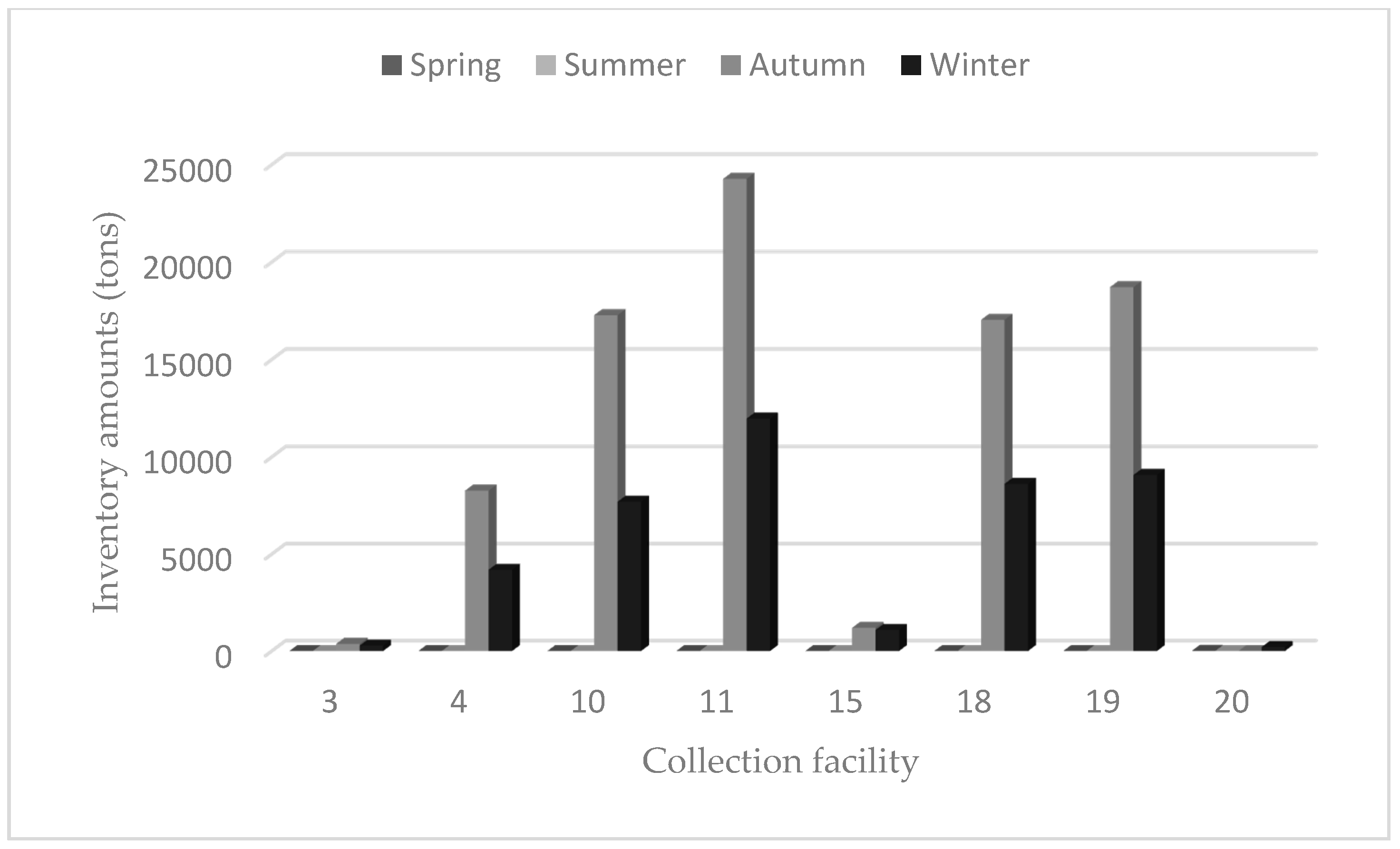
4.2. Impact of Seasonality and Disruption Risk

The traditional design of biomass supply chain network rarely takes disruption risks into account. To demonstrate the impact of seasonality and disruption risks, we design the NE Biofuel Company case using a traditional model (i.e., which does not consider the disruption risk or feedstock seasonality), and then we test the performance of these resulting designs in the real world (i.e., where disruption risks do exist). When the disruption risk is not considered, each farmer is assigned to one facility and there is no penalty cost. When the feedstock seasonality is not considered, we assume that farmers produce the same amount of feedstock in each season equal to the average of the production across seasons. Figure 9a–d depict the optimal facility location design for each of the four cases (with or without disruption risk, with or without feedstock seasonality).

The disruption risk and feedstock seasonality both have a significant impact on the optimal facility location design. In the first case (with disruption risk and with feedstock seasonality), eight collection facilities are built to hedge against the disruption risk. For example, while the facility at Location 3 only serves one farmer as the primary facility, it serves eight farmers as their first backup facility. These backup allocations can help the biofuel company to maintain reliability even if some of the facilities fail. In Figure 9b, fewer facilities are built as compared to the case under disruption risk. Because collection facilities are no longer subject to the disruption risk, each farmer is assigned to only one facility. Thus, the biofuel company can reduce the number of collection facilities. To study the impact of feedstock seasonality, we compare Figure 9c with Figure 9a, and Figure 9d with Figure 9b. We observe that the optimal locations are the same, respectively, but the allocations of the farmers have quite changed. In Figure 9c, the facility at location 3 is no longer serving any farmer as his primary facility and in Figure 9d, Farmers #1, #9, #14 are abandoned with no service. These changes in facilities allocations are due to the clear feedstock variability and inventory balancing considerations.

The computational results of the abovementioned four cases are summarized in

Table 3. Solutions statistics for the four cases.

Case		Facility Location	Objective ($M)	Evaluated Cost under Disruption ($M)	Cost Difference (%)	Inventory Cost ($M)
Disruption	Seasonality
Yes	Yes	3, 4, 10, 11, 15, 18, 19, 20	5.65	5.65	0	1
No	Yes	4, 10, 11, 18, 19	5.41	6.56	17.5	0.99
Yes	No	3, 4, 10, 11, 15, 18, 19, 20	4.64	4.64	0	0.003
No	No	4, 10, 11, 18, 19	4.38	5.68	22.8	0

. For each case, we list the optimal objective value from the respective model (e.g., ignoring disruption risk or feedstock seasonality), the evaluated cost assuming that disruption risk does exist, as well as the inventory cost. It is obvious that with the traditional solution, the cost under a disruption-free scenario is $5.41 million while the cost under a realistic disruption scenario is $6.56 million. When using our reliable solution, the cost under a realistic disruption scenario can be reduced to $5.56 million. Comparing the first case with the third case, we find that the total cost increased from $4.64 million to $5.65 million under feedstock seasonality.

In summary, we find that: (1) the disruption risk of collection facilities affects both optimal facility deployment and the supply chain cost; (2) it is worth investing more collection facilities to mitigate the negative impact of disruption risk and the optimal locations tend to be at places with high biomass supply; (3) the feedstock seasonality will not directly affect locations of the collection facilities, but it will affect the allocation of collection facilities and bring higher inventory cost for the biomass supply chain.

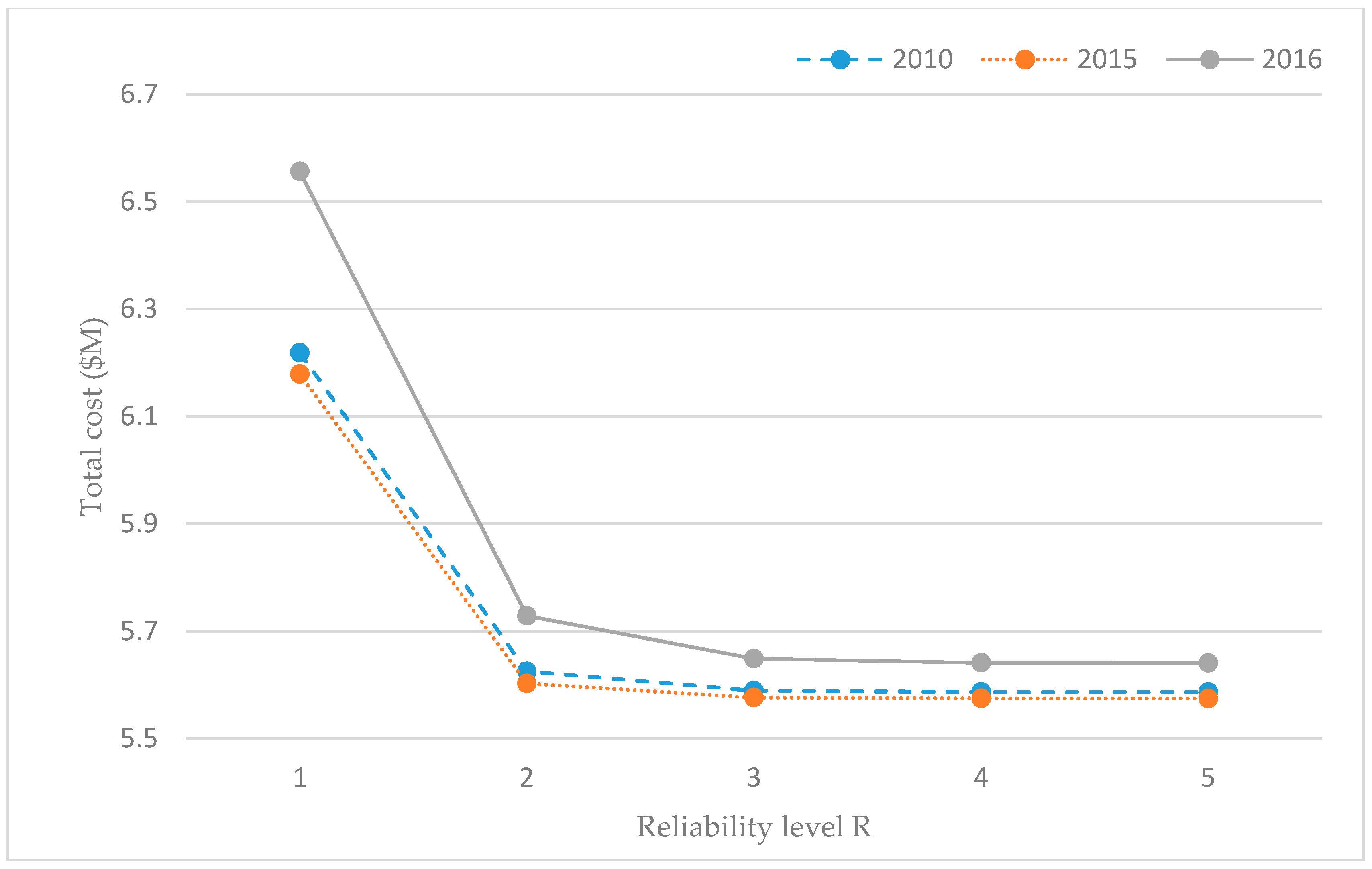
4.3. Impact of Failure Probability and Reliability Level

In this paper, we use rainfall data and damage area caused by floods to estimate the disruption risk of the collection facility. Thus, the failure probability of the facility shows significant seasonality. To test the impact of failure probability, we select different flood data and rainfall data in 2015 and 2010 to evaluate the failure probability. Now we test other failure probabilities as follows: ${\mathrm{q}}_{2015}=(0.02,0.03,0.02,0.01)$, ${\mathrm{q}}_{2010}=(0.03,0.04,0.01,0.02)$, using single-year data. The costs are presented in Figure 10. The results show that the total cost of supply chain is positively correlated to the failure probability. We also observe that no matter how the failure probability changes, setting backup facilities (R >1) can significantly decrease the total cost. It demonstrates that the reliable network performs better than a traditional network under disruption risk.

Table 4. Cost with different reliability level in 2016.

Reliability Level	Facility Locations	Fixed Cost ($M)	Transportation Cost ($M)	Inventory Cost ($M)	Total Cost ($M)
1	4, 10, 11, 18, 19	0.23	5.38	0.94	6.55
2	3, 4, 10, 11, 15, 18, 19, 20	0.37	4.36	0.99	5.72
3	3, 4, 10, 11, 15, 18, 19, 20	0.37	4.28	1	5.65
4	3, 4, 10, 11, 15, 18, 19, 20	0.37	4.27	1	5.64
5	3, 4, 10, 11, 15, 18, 19, 20	0.37	4.26	1	5.63

shows the solution of the model with different reliability levels in 2016. When the company employs the traditional allocation strategy, in which the farmer is always served by one certain facility, only five collection facilities are set with low fixed cost and inventory cost but high transportation cost and total cost. When the company employs the backup facilities strategy, in which each farmer is assigned to one primary facility and several backup facilities, the company builds eight facilities with high fixed cost and inventory cost but low transportation cost and total cost. The result demonstrates that when considering disruption risks, the higher reliability level network performs much better than the lower level network because the backup facilities can maintain the operation of the supply chain even if some of facilities in the network failed. It is worth pointing out that regardless of the value of the reliability level, the model returned the same set of facility locations (eight facilities), although a higher reliability level in general helps to reduce the total cost.

5. Discussion and Conclusions

This paper studied a reliable biomass supply chain design against seasonal variations of feedstock and probabilistic disruptions of collection facilities. We formulated an integrated multi-period supply chain model in which the available feedstock production and disruption risks both vary seasonally. Our model was applied to determine optimal collection facility locations, allocations, inventories, and feedstock quantity. A real-world case in Hubei, China was developed to test the model. Several numerical experiments were conducted to analyze the impacts of facility disruptions and feedstock seasonality on the biomass supply chain.

A lot of studies in recent years have focused on exploring the influences of probabilistic facility disruptions on the supply chain, but most of the work considered a static two-stage supply chain [29,30]. Only a few of such studies (e.g., Marufuzzaman et al. [25] and Bai et al. [38]) considered facility disruptions in biomass supply chains, and furthermore, it seems that no research has simultaneously considered biomass feedstock seasonality and collection facility disruption risks. In this paper, we formulated a three-stage multi-period design model for biomass supply chain under feedstock seasonality and probabilistic facility disruptions. Thus, the output of our model provides more sophisticated and more realistic decisions for the biomass company. The case study shows that while achieving reliable design would typically lead to more collection facilities (incurring more fixed investment cost), it could definitely reduce the expected transportation and inventory costs under disruption risks, and in turn reduce the overall system-wide expected cost. Furthermore, our computation results further verify that, in three echelons biomass supply chains with inventory considerations as well as location-dependent disruption probabilities, it may be sub-optimal to assign farmers to service facilities based on distance proximity.

In the numerical experiments, similar to Bai, et al. [38], we compared our reliable solution with a deterministic solution which considered only the disruption-free scenario. It was found that disruption risks significantly affect both the optimal facility locations and the supply chain cost. Furthermore, we further investigated the impacts of feedstock seasonality. It was found that the feedstock seasonality does not directly affect locations of the collection facilities, but it affects the allocation of collection facilities and brings higher inventory cost for the biomass supply chain. We also discussed the impact of failure probability and maximum backup level on the biomass supply chain. We found out that the total cost of the supply chain is positively correlated with the failure probability. The model returned the same set of facility locations regardless of the value of the maximum backup level, although a higher maximum back up level in general helps reduce the total expected cost.

Our findings also bring up new questions for future research. First, in this paper, we assumed that the capacity of collection facilities is infinite. In order to develop more realistic insights, future research could relax this assumption by considering finite capacity limits. Second, we assume that the failure probability of facilities stays the same across locations (although they vary across seasons). However, in reality, the failure probability is likely to vary across different locations. Finally, many real-world facility disruptions exhibit spatial and temporal correlations; future research may attempt to consider correlated facility disruptions.

References

1. Perlack, R.D.; Wright, L.L.; Turhollow, A.F.; Graham, R.L.; Stokes, B.J.; Erbach, D.C. Biomass as Feedstock for a Bioenergy and Bioproducts Industry: The Technical Feasibility of a Billion-Ton Annual Supply; Oak Ridge National Labboratory: Oak Ridge, TN, USA, 2005.
2. Ebadian, M. Design and Scheduling of Agricultural Biomass Supply Chain for a Cellulosic Ethanol Plant. Ph.D. Thesis, University of British Columbia, Vancouver, BC, Canada, 2013. [Google Scholar]
3. Yue, D.; You, F.; Snyder, S.W. Biomass-to-bioenergy and biofuel supply chain optimization: Overview, key issues and challenges. Comput. Chem. Eng. 2014, 66, 36–56. [Google Scholar] [CrossRef]
4. Iakovou, E.; Karagiannidis, A.; Vlachos, D.; Toka, A.; Malamakis, A. Waste biomass-to-energy supply chain management: A critical synthesis. Waste Manag. 2010, 30, 1860–1870. [Google Scholar] [CrossRef] [PubMed]
5. Zhou, J.; Wu, H.; Ding, S.; Zhu, C. Analysis of seasonality and sustainability of straw resources. Resour. Sci. 2011, 33, 1537–1545. [Google Scholar]
6. Li, X.P.; Ouyang, Y.F. A continuum approximation approach to reliable facility location design under correlated probabilistic disruptions. Transp. Res. Part B Methodol. 2010, 44, 535–548. [Google Scholar] [CrossRef]
7. Rentizelas, A.A.; Tolis, A.J.; Tatsiopoulos, I.P. Logistics issues of biomass: The storage problem and the multi-biomass supply chain. Renew. Sustain. Energy Rev. 2009, 13, 887–894. [Google Scholar] [CrossRef] [Green Version]
8. Ekşioğlu, S.D.; Acharya, A.; Leightley, L.E.; Arora, S. Analyzing the design and management of biomass-to-biorefinery supply chain. Comput. Ind. Eng. 2009, 57, 1342–1352. [Google Scholar] [CrossRef]
9. Chen, C.W.; Fan, Y.Y. Bioethanol supply chain system planning under supply and demand uncertainties. Transp. Res. Part E Logist. Transp. Rev. 2012, 48, 150–164. [Google Scholar] [CrossRef]
10. Xie, F.; Huang, Y.X.; Eksioglu, S. Integrating multimodal transport into cellulosic biofuel supply chain design under feedstock seasonality with a case study based on California. Bioresour. Technol. 2014, 152, 15–23. [Google Scholar] [CrossRef] [PubMed]
11. Huang, Y.X.; Fan, Y.Y.; Chen, C.W. An integrated biofuel supply chain to cope with feedstock seasonality and uncertainty. Transp. Sci. 2014, 48, 540–554. [Google Scholar] [CrossRef]
12. Pettersson, K.; Wetterlund, E.; Athanassiadis, D.; Lundmark, R.; Ehn, C.; Lundgren, J.; Berglin, N. Integration of next-generation biofuel production in the Swedish forest industry—A geographically explicit approach. Appl. Energy 2015, 154, 317–332. [Google Scholar] [CrossRef]
13. Ouraich, I.; Lundmark, R. A geographically explicit approach for price determination of forest feedstock under different next-generation biofuel production scenarios-the case of Sweden. In Proceedings of the Swedish Association for Energy Economics Conference on Meeting Sweden’s Current and Future Energy Challenges, Luleå, Sweden, 23–24 August 2016. [Google Scholar]
14. Nasiri, F.; Mafakheri, F.; Adebanjo, D.; Haghighat, F. Modeling and analysis of renewable heat integration into non-domestic buildings—The case of biomass boilers: A whole life asset-supply chain management approach. Biomass Bioenergy 2016, 95, 244–256. [Google Scholar] [CrossRef]
15. Huang, Y.X.; Chen, C.W.; Fan, Y.Y. Multistage optimization of the supply chains of biofuels. Transp. Res. Part E Logist. Transp. Rev. 2010, 46, 820–830. [Google Scholar] [CrossRef]
16. Dal-Mas, M.; Giarola, S.; Zamboni, A.; Bezzo, F. Strategic design and investment capacity planning of the ethanol supply chain under price uncertainty. Biomass Bioenergy 2011, 35, 2059–2071. [Google Scholar] [CrossRef]
17. You, F.; Wang, B. Life cycle optimization of biomass-to-liquid supply chains with distributed–centralized processing networks. Ind. Eng. Chem. Res. 2011, 50, 10102–10127. [Google Scholar] [CrossRef]
18. Walther, G.; Schatka, A.; Spengler, T.S. Design of regional production networks for second generation synthetic bio-fuel—A case study in Northern Germany. Eur. J. Oper. Res. 2012, 218, 280–292. [Google Scholar] [CrossRef]
19. Akgul, O.; Shah, N.; Papageorgiou, L.G. An optimisation framework for a hybrid first/second generation bioethanol supply chain. Comput. Chem. Eng. 2012, 42, 101–114. [Google Scholar] [CrossRef]
20. Gautam, S.; LeBel, L.; Carle, M.A. Supply chain model to assess the feasibility of incorporating a terminal between forests and biorefineries. Appl. Energy 2017, 198, 377–384. [Google Scholar] [CrossRef]
21. Marufuzzaman, M.; Ekşioğlu, S.D. Managing congestion in supply chains via dynamic freight routing: An application in the biomass supply chain. Transp. Res. Part E Logist. Transp. Rev. 2017, 99, 54–76. [Google Scholar] [CrossRef]
22. Tang, C.S. Perspectives in supply chain risk management. Int. J. Prod. Econ. 2006, 103, 451–488. [Google Scholar] [CrossRef]
23. Ivanov, D.; Pavlov, A.; Dolgui, A.; Pavlov, D.; Sokolov, B. Disruption-driven supply chain (re)-planning and performance impact assessment with consideration of pro-active and recovery policies. Transp. Res. Part E Logist. Transp. Rev. 2016, 90, 7–24. [Google Scholar] [CrossRef]
24. Peng, M.; Peng, Y.; Chen, H. Post-seismic supply chain risk management: A system dynamics disruption analysis approach for inventory and logistics planning. Comput. Oper. Res. 2014, 42, 14–24. [Google Scholar] [CrossRef]
25. Marufuzzaman, M.; Eksioglu, S.D.; Li, X.; Wang, J. Analyzing the impact of intermodal-related risk to the design and management of biofuel supply chain. Transp. Res. Part E Logist. Transp. Rev. 2014, 69, 122–145. [Google Scholar] [CrossRef]
26. Gedik, R.; Medal, H.; Rainwater, C.; Pohl, E.A.; Mason, S.J. Vulnerability assessment and re-routing of freight trains under disruptions: A coal supply chain network application. Transp. Res. Part E Logist. Transp. Rev. 2014, 71, 45–57. [Google Scholar] [CrossRef]
27. Snyder, L.V.; Daskin, M.S. Reliability models for facility location: The expected failure cost case. Transp. Sci. 2005, 39, 400–416. [Google Scholar] [CrossRef]
28. Berman, O.; Krass, D.; Menezes, M.B. Facility reliability issues in network p-median problems: Strategic centralization and co-location effects. Oper. Res. 2007, 55, 332–350. [Google Scholar] [CrossRef]
29. Cui, T.T.; Ouyang, Y.F.; Shen, Z.J.M. Reliable facility location design under the risk of disruptions. Oper. Res. 2010, 58, 998–1011. [Google Scholar] [CrossRef]
30. Lim, M.; Daskin, M.S.; Bassamboo, A.; Chopra, S. A facility reliability problem: Formulation, properties, and algorithm. Nav. Res. Logist. 2010, 57, 58–70. [Google Scholar] [CrossRef]
31. Shen, Z.-J.M.; Zhan, R.L.; Zhang, J. The reliable facility location problem: Formulations, heuristics, and approximation algorithms. INFORMS J. Comput. 2011, 23, 470–482. [Google Scholar] [CrossRef]
32. Chen, Q.; Li, X.P.; Ouyang, Y.F. Joint inventory-location problem under the risk of probabilistic facility disruptions. Transp. Res. Part B Methodol. 2011, 45, 991–1003. [Google Scholar] [CrossRef]
33. Lim, M.K.; Bassamboo, A.; Chopra, S.; Daskin, M.S. Facility location decisions with random disruptions and imperfect estimation. Manuf. Serv. Oper. Manag. 2013, 15, 239–249. [Google Scholar] [CrossRef]
34. Xie, W.J.; Ouyang, Y.F.; Wong, S.C. Reliable location-routing design under probabilistic facility disruptions. Transp. Sci. 2016, 50, 1128–1138. [Google Scholar] [CrossRef]
35. Hasani, A.; Khosrojerdi, A. Robust global supply chain network design under disruption and uncertainty considering resilience strategies: A parallel memetic algorithm for a real-life case study. Transp. Res. Part E Logist. Transp. Rev. 2016, 87, 20–52. [Google Scholar] [CrossRef]
36. Khosrojerdi, A.; Zegordi, S.H.; Allen, J.K.; Mistree, F. A method for designing power supply chain networks accounting for failure scenarios and preventive maintenance. Eng. Optim. 2016, 48, 154–172. [Google Scholar] [CrossRef]
37. Zhao, M.; Cui, J.; Li, X.; Parsafard, M.; An, S. A Reliable Model for Integrated Supply Chain Design under Disruption Risk. In Proceedings of the 95th Annual Meeting on Transportation Research Board, Washington, DC, USA, 10–14 January 2016. [Google Scholar]
38. Bai, Y.; Li, X.P.; Peng, F.; Wang, X.; Ouyang, Y.F. Effects of disruption risks on biorefinery location design. Energies 2015, 8, 1468–1486. [Google Scholar] [CrossRef]
39. Sherali, H.D.; Alameddine, A. A new reformulation-linearization technique for bilinear programming problems. J. Glob. Optim. 1992, 2, 379–410. [Google Scholar] [CrossRef]
40. Bureau of Stastics of the Hubei Province. Hubei Stastical Yearbook 2016; China Statistics Press: Beijing, China, 2016; pp. 120–121.
41. National Bureau of Stastics of the People’s Republic of China. China Stastical Yearbook 2015; China Statistics Press: Beijing, China, 2015; pp. 184–185.
42. National Bureau of Stastics of the People’s Republic of China. China Stastical Yearbook 2016; China Statistics Press: Beijing, China, 2016; pp. 186–187.
43. National Bureau of Stastics of the People’s Republic of China. China Stastical Yearbook 2014; China Statistics Press: Beijing, China, 2014; pp. 175–176.
44. National Bureau of Stastics of the People’s Republic of China. China Stastical Yearbook 2013; China Statistics Press: Beijing, China, 2013; pp. 182–183.
45. National Bureau of Stastics of the People’s Republic of China. China Stastical Yearbook 2012; China Statistics Press: Beijing, China, 2012; pp. 183–184.
46. National Bureau of Stastics of the People’s Republic of China. China Stastical Yearbook 2011; China Statistics Press: Beijing, China, 2011; pp. 178–179.
47. National Bureau of Stastics of the People’s Republic of China. China Stastical Yearbook 2010; China Statistics Press: Beijing, China, 2010; pp. 173–174.
Figure 1. Biomass supply chain structure.
Energies 10 01895 g001
Figure 2. Fraction of a supply network.
Energies 10 01895 g002
Figure 3. Geographical distributions of farmers in Hubei Province, China.
Energies 10 01895 g003
Figure 4. Geographical distributions of collection facilities and refineries.
Energies 10 01895 g004
Figure 5. Historical rainfall of Hubei Province.
Energies 10 01895 g005
Figure 6. Facility locations and assignments. (a) Level 0 assignments; (b) Level 1 assignments; (c) Level 2 assignments.
Energies 10 01895 g006
Figure 7. Feedstock amount from farmers.
Energies 10 01895 g007
Figure 8. Inventory in the collection facilities.
Energies 10 01895 g008
Figure 9. Optimal facility locations for the four cases. (a) Disruption risk and feedstock seasonality; (b) Disruption risk free and feedstock seasonality; (c) Disruption risk and feedstock stability; (d) Disruption risk free and feedstock stability.
Energies 10 01895 g009
Figure 10. Cost with different failure probability.
Energies 10 01895 g010