Novel Strategy for Accurate Locating of Voltage Sag Sources in Smart Distribution Networks with Inverter-Interfaced Distributed Generators

Abstract

With the aid of power quality monitoring systems (PQMSs), accurate locating of voltage sag sources, which has important significance for guiding maintenance personnel in finding and repairing faults as well as improving power supply reliability, has been becoming a new research hotspot. However, existing methods have unsatisfactory locating accuracy due to the integration of distributed generators (DGs) and fault resistance. In this paper, a novel strategy for accurately locating voltage sag sources in smart distribution networks is proposed. Based on inverse theory, which is well applied in geophysics, the accurate location issue is treated as a two-step optimization model. It aims at making the distribution of voltage phasors and current phasors obtained by theoretical short-circuit calculation match those actually observed as closely as possible. To guarantee the feasibility of the strategy, the effect of inverter-interfaced DGs (IIDGs) which are the main form of DG is considered in the short-circuit calculations. To guarantee the location accuracy of the strategy, fault resistance is treated as an optimization variable in the two-step optimization model to eliminate estimation error of fault resistance. Via two modified IEEE benchmarks with different scales, the validity and the superiorities in applicability and accuracy of the proposed strategy are verified.

1. Introduction

As one of the most important power quality (PQ) issues, voltage sags can cause misoperation and even damage to equipment, and further affect the normal operation of power systems [1,2,3]. In recent years, analyses of voltage sag on the basis of data collected from widely applied PQ monitoring system (PQMSs) have been becoming a new research hotspot.

For the detection and cause identification of voltage sag events, several available methods have been proposed. In [4], three Kalman filters were proposed to accurately detect when a voltage event begins and to estimate the three-phase voltage supply during the event. References [5,6] proposed to use the fuzzy rule and support vector machine (SVM) to identify whether the sag event is caused by short-circuit faults, respectively.

Short-circuit faults are the most common causes of voltage sag. After real-time operation of protective relay systems, fault locating is typically a non-real time application for which the accuracy is the main objective [7]. Accurate location of voltage sags caused by short-circuit faults has important significance for guiding the maintenance personnel to find and repair faults as well as improving the reliability of the power supply.

The impedance-based methods and traveling wave-based methods show good fault location performance in transmission networks. When these methods are applied to distribution networks, a large amount of phase-voltage transformers (PTs)/current transformers (CTs) or devices which can realize fault-distance-measuring are needed. Therefore, the costs of these devices and the corresponding communication systems in the application of the methods are quite high. A series of publications concentrate on locating the voltage sag source based on the measurement data obtained by sparse PQ observation points. In detail, they can be classified into two categories.

(1)

Rough locating to get potential/candidate areas [8,9,10,11,12]. The methods of this category can judge the upstream or downstream relationship of sag sources related to each observation point via the measured information. Reference [8] proposed a method using the disturbance of active power before and after the sag and the disturbance energy, which is the integral of the disturbance of active power during the sag. In [9], via voltage and current phasors and power factor, a method based on the slope of a line which is obtained by least squares fitting approach was put forward. The method using the polarity of the real current component was presented in [10]. Reference [11] put forward a method using real part sign of the measured fundamental positive-sequence impedance. In [12], a method using the fault components based instantaneous active- and reactive-energy was proposed. Combining with the information of topology and locations of observation points in the network, potential/candidate area of voltage sag source can be roughly determined with these methods.

(2)

Accurate locating. In [7,13,14], methods which can accurately locate of voltage sag caused by short-circuit fault in traditional radial distribution networks were proposed. The common core concept of these methods is to realize the best match between the actually observed data and theoretically calculated data. Among them, reference [7] is the most representative, with the best locating performance. In detail, the fault resistance of each node is estimated using the current at the root node, one by one. Then, the node with the minimum error between the calculated voltages and those actually observed at the sparse PQ observation points is identified as the faulted node. Further, the fault resistance estimated at the faulted node is used to find the accurate fault location by traversing all the branches connected to the faulted node.

With the wide integration of DGs, especially inverter interfaced DGs (IIDGs) which are the main form of DGs, smart distribution networks have been transformed into active complex networks with two or more power supplies. Consequently, the load flows and distribution of short-circuit currents in smart distribution networks are becoming more complex than in the traditional distribution network [15,16]. Thus, in smart distribution networks, fault resistance can no longer be simply estimated with the information at the root node. Furthermore, when the short-circuit fault occurs at a branch rather than a node, the faulted node is not the accurate fault location. Namely, there exists a difference between the estimated fault resistance and the actual fault resistance. This error may affect the precision of short-circuit calculation and further result in negative impacts on the locating accuracy.

To realize accurate locating of voltage sag sources caused by short-circuit faults in smart distribution networks, a novel strategy is proposed with the aid of PQMS and Distribution Automation System (DAS). Based on the inverse theory, by minimizing the differences between the calculated phasors of voltages and currents and those actually observed, a two-step optimization model is established to in turn locate the nearest node relative to fault and accurate fault location. To guarantee the feasibility, short-circuit calculation method of smart distribution network considering the effects of IIDGs is analyzed. Moreover, to improve locating accuracy, fault resistance is optimized twice in the two-step optimization model to eliminate the side effects on locating accuracy caused by the estimation error of fault resistance.

The remainder of the paper is structured as follows. In Section 2, the two-step optimization model for accurate locating is proposed based on inverse theory. Short-circuit calculation method considering the effects of IIDGs is analyzed in Section 3. The framework of the proposed locating strategy is given in Section 4. Performances of the proposed strategy are demonstrated via a modified IEEE 33-node benchmark and a modified IEEE 69-node benchmark in Section 5. Discussions of the obtained results are given in Section 6.

2. Two-Step Optimization Model for Accurate Locating Based on Inverse Theory

As pointed out in the Introduction, studies about the detection and cause identification of voltage sag events as well as candidate area derivation of sag sources are available. Therefore, this paper focuses on the issue of accurate locating. Different from traditional distribution networks, smart distribution networks are active complex networks with multiple power supplies. Thus, analyses based on the characteristics of the traditional distribution network may no longer be suitable for smart distribution networks. To realize accurate locating of voltage sags caused by short-circuit faults in smart distribution networks, a concept based on inverse theory is proposed.

2.1. Brief Introduction of Inverse Theory

The solution of inverse problems involves the retrieval of information about a physical process or phenomenon from known or observed data [17]. It is well applied in reconstructing the internal structure of the Earth from a finite set of remotely observed data.

The definition of general forward and inverse problems can be described schematically as illustrated in the chart of Figure 1 [18]. The forward problem is to predict the observed data for given parameters with certain functional relation. While the inverse problem is to reconstruct the parameters from the actual observed data:

The forward problem can be represented as (1):

$${\mathit{d}}_{syn}=g(\mathit{m})$$

(1)

where g is a forward modeling operator, which operates on the vector of parameters m to generate synthetic/predicted data vector d_syn.

The solution to the inverse problem is to find a m_pr that makes d_syn “fits-well” the actual observed data d_obs [19]. Therefore, the inverse problem is often cast as minimization of the data error ∆d = d_obs − d_syn as follows:

$$\min ({\Vert \Delta d\Vert }_a={\left[{\displaystyle \sum _{i=1}^N{\left|\Delta d_i\right|}^a}\right]}^{1/a}$$

(2)

where a is an integer, which represents the order of the norm. Common used values of a are 1 and 2.

In accurate locating of voltage sag caused by short-circuit fault, the forward modeling operator g is short-circuit calculation method; m is the hypothetical fault information including fault location and fault resistance; a is selected as 1.

Based on inverse theory, a two-step optimization model is proposed, which aims at making the distribution of voltage phasors and current phasors obtained by theoretical short-circuit calculation match those actually observed as closely as possible:

(1)

The first-step of the optimization model is to search the nearest node (denoted as ne-node) relative to the fault point in the candidate area set1. The ne-node is the node, which can achieve the best match of voltage phasors and current phasors between those actually observed and obtained theoretically with appropriate fault resistance. Further, the candidate set of faulted branch (denoted as set2), can be obtained as the branches connected with ne-node.

(2)

The second-step of the optimization model is to locate the accurate fault point in set2. By establishing two-step optimization model, the search space can be reasonably decomposed. As the result, accurate locating is carried out just in set2 rather than all the branches in set1. A detailed illustration of the two-step optimization model is as follows:

2.2. The First-Step for Searching the Nearest Node

On the basis of inverse theory, the first-step of the two-step optimization model for searching ne-node can be established as follows.

2.2.1. Optimization Variables

There are two optimization variables of the faulted node b (b∈set1) and fault resistance r_f1. b is discrete, while r_f1 is continuous.

2.2.2. Objective Function

Specifically, the purpose is to find the optimal b (namely the ne-node) and r_f1 to minimize the objective function (3):

$$f1=\min {\displaystyle \sum _{h=1}^n{\displaystyle \sum _{p=A,B,C}(\left|u_{hp}{}^{ca}(b,r_{f1})-u_{hp}{}^{obs}\right|}+{\displaystyle \sum _{s=1}^{m_h}\left|i_{hsp}{}^{ca}(b,r_{f1})-i_{hsp}{}^{obs}\right|})}$$

(3)

where u_hp^ca(b,r_f1) and i_hsp^ca(b,r_f1) are the theoretically calculated voltage phasor and current phasor of phase p at observation point h, when the fault occurs at node b with fault resistance r_f1. u_hp^obs and i_hsp^obs are the observed voltage phasor and current phasor of phase p at observation point h. n is the total number of observation points. m_h is the total number of the branches connected with observation point h.

2.2.3. Constraints

Specifically, there are two constraints as listed in (4).

(1)

Faulted node b should be one node in set1.

(2)

Fault resistance r_f1 should in allowable range.

$$\{\begin{array}{l}b\in \mathit{set1}\\ 0\le r_{f1}\le r_{max}\end{array}$$

(4)

where r_max is the upper limit value of r_f1.

2.2.4. Solution

For the above discrete-continuous mixed optimization model, the hybrid particle swarm optimization (HPSO) algorithm [20], with high efficiency and good convergence, is used to search the optimal solution. The HPSO algorithm is consisted of three kinds of variants, which are continuous variables, discrete variables and binary variables. Further, fuzzy adaptive inference is introduced to avoid the algorithm being trapped in the local optima prematurely.

2.3. The Second-Step for Searching the Accurate Location

For short-circuit faults that occur at a branch rather than a node, the ne-node will be one end of the branch. As the ne-node is not the accurate fault location, there will be an error between the optimal r_f1 obtained in the first-step optimization and the actual fault resistance. Therefore, the fault resistance should be re-optimized in the second-step of the two-step optimization model. On the basis of inverse theory, the second-step of the two-step optimization model for searching the accurate location can be established as follows.

2.3.1. Optimization Variables

There are three optimization variables:

(1)

The faulted branch l;

(2)

The relative distance λ (0 ≤ λ ≤ 1) between the fault point and the head of faulted branch;

(3)

Fault resistance r_f2.

Specifically, l is discrete, while λ and r_f2 are continuous.

As shown in Figure 2, the relative distance λ is defined as follows (5):

$$\lambda =\frac{L_{pf}}{L_{pq}}$$

(5)

where L_pf is the length between node p and fault point f, L_pq is the length between node p and node q.

2.3.2. Optimization Variables

Specifically, the aim is to find the optimal l, λ and r_f2 to minimize the objective function (6):

$$f2=\min {\displaystyle \sum _{h=1}^n{\displaystyle \sum _{p=A,B,C}(\left|u_{hp}{}^{ca}(l,\lambda ,r_{f2})-u_{hp}{}^{obs}\right|}+{\displaystyle \sum _{s=1}^{m_h}\left|i_{hsp}{}^{ca}(l,\lambda ,r_{f2})-i_{hsp}{}^{obs}\right|})}$$

(6)

where u_hp^ca(l,λ,r_f2) and i_hsp^ca(l,λ,r_f2) are the theoretically calculated voltage phasor and current phasor of phase p at observation point h, when the fault occurs at branch l with relative distance λ and fault resistance r_f2.

2.3.3. Constraints

Specifically, there are three constraints as listed in (7).

(1)

Faulted branch l should be one branch in set2.

(2)

Relative distance λ should be in [0, 1].

(3)

Fault resistance r_f2 should in allowable range.

$$\{\begin{array}{l}l\in \mathit{set2}\\ 0\le \lambda \le 1\\ 0\le r_{f2}\le r_{max}\end{array}$$

(7)

where λ equals to 0 means the fault locates at the head of l, while λ equals to 1 means the fault locates at the end of l; r_max is the upper limit of r_f2.

2.3.4. Solution

As the above model is also a discrete-continuous mixed optimization model, the HPSO algorithm is again used to search the optimal solution.

3. Short-Circuit Calculation of Smart Distribution Network with IIDGs

Accurate short circuit calculation methods are the basis to realize accurate locating. The distribution of short circuit currents and voltages in smart distribution networks with DGs is more complex than in traditional radial distribution networks.

As the main form of DG, IIDG has different characteristic of short-circuit current with synchronous generator [21,22,23]. It contributes less fault current than a traditional rotating machine. Fault response rate of IIDG is very fast and short-circuit characteristic mainly depends on the control strategy. Therefore, to guarantee the applicability of the proposed strategy to smart distribution network with IIDGs, short circuit calculation considering IIDGs should be analyzed. In this section, the short circuit characteristic of IIDG and corresponding effects on the short circuit calculation of distribution network are analyzed, respectively.

3.1. Voltage-Controlled Positive Sequence Current Source Model of IIDG under Fault

In [22], a control strategy for low voltage ride-through of IIDG was proposed and the fault current characteristics of IIDG under different fault conditions were studied. It was summarized that IIDG can always be treated as a voltage-controlled positive-sequence current source under symmetrical fault or asymmetrical fault [22,23] with adequate phase lock loop (PLL) [24]. As shown in Figure 3, if an IIDG interfaces with node i, ${\dot{V}}_{i\left(1\right)}={\alpha }_i\angle {\phi }_{vi}$ is the positive-sequence terminal voltage.

The equivalent positive-sequence current source ${\dot{I}}_{IIDGi}=I_i\angle {\phi }_{ci}$ of the IIDG can be specifically expressed as follows:

(1)

If ${\alpha }_i>0.9$, then $I_i=i_{d0i}^{*}$, and ${\phi }_{ci}={\phi }_{vi}$.

(1)

If $0.4\le {\alpha }_i\le 0.9$ and $2(1-{\alpha }_i)\le \sqrt{{1.2}^2-{(i_{d0i}^{*})}^2}$, then $I_i\le \sqrt{{(i_{d0i}^{*})}^2+4{(1-{\alpha }_i)}^2}$ and ${\phi }_{ci}={\phi }_{vi}+{\tan }^{-1}\left[2(1-{\alpha }_i)/i_{d0i}^{*}\right]$.

(3)

If $0.4\le {\alpha }_i\le 0.9$ as well as $2(1-{\alpha }_i)>\sqrt{{1.2}^2-{(i_{d0i}^{*})}^2}$, then $I_i=1.2$ and ${\phi }_{ci}={\phi }_{vi}+{\tan }^{-1}[2(1-{\alpha }_i)/\sqrt{{1.2}^2+4{(1-{\alpha }_i)}^2}]$.

(4)

If ${\alpha }_i<0.4$, then $I_i=1.2$ and ${\phi }_{ci}={\phi }_{vi}+90°$.

$i_{d0i}^{*}$ is the per-unit reference value of active current of IIDG before fault occurrence. ${\alpha }_i$ and $I_i$ are the per-unit voltage magnitude and current magnitude. ${\phi }_{vi}$ and ${\phi }_{ci}$ are the voltage phase and current phase.

3.2. Short-Circuit Calculation of Smart Distribution Network with IIDGs

According to the above analyses, IIDGs only affect fault analysis of positive-sequence network.

For a network before fault occurrence, the normal positive sequence voltage of node i can be represented as (8):

$${\dot{V}}_{i(1)}^0={\displaystyle \sum _{j\in G_1}{Z}_{ij}{\dot{I}}_j}$$

(8)

where G₁ is the set of all active nodes, including integration points of IIDGs; Z_ij is the positive sequence mutual impedance between node i and node j; İ_j is the positive sequence injection current of each active node.

If an IIDG interfaced with node k, there should be an equivalent controlled current source ∆İ_DGk in positive sequence super-imposed network:

$$\Delta {\dot{I}}_{DGk}={\dot{I}}_{DGk}-{\dot{I}}_{DGk0}$$

(9)

where İ_DGk0 and İ_DGk are the output positive sequence currents of the IIDG before and after fault occurrence, respectively.

Thus, positive-sequence fault component of the voltage of node i should be as (10):

$$\Delta {\dot{V}}_{i(1)}^{}={\displaystyle \sum _{k\in G_2}{Z}_{ik}\Delta {\dot{I}}_{DGk}}-Z_{if}{\dot{I}}_{f(1)}$$

(10)

where G₂ only contains the access points of IIDGs. Z_ik is the positive sequence mutual impedance between node i and node k, while Z_if is the positive sequence mutual impedance between node i and fault point f. İ_f(1) is the positive sequence fault current.

The actual positive-sequence voltage of node i after fault occurrence is as follows:

$$\begin{array}{ll}{\dot{V}}_{i(1)}^{}& ={\dot{V}}_{i(1)}^0+\Delta {\dot{V}}_{i(1)}^{}\hfill \\ & ={\dot{V}}_{i(1)}^0+{\displaystyle \sum _{k\in G_2}{Z}_{ik}\Delta {\dot{I}}_{DGk}}-Z_{if}{\dot{I}}_{f(1)}\hfill \end{array}$$

(11)

Furthermore, actual positive-sequence voltages of each IIDG interfaced node p (p ∈ G₂) and fault point f can be expressed as Equations (12) and (13), respectively:

$$\begin{array}{ll}{\dot{V}}_{p(1)}^{}& ={\dot{V}}_{p(1)}^0+\Delta {\dot{V}}_{p(1)}^{}\hfill \\ & ={\dot{V}}_{p(1)}^0+{\displaystyle \sum _{k\in G_2}{Z}_{pk}\Delta {\dot{I}}_{DGk}}-Z_{if}{\dot{I}}_{f(1)}\hfill \end{array}$$

(12)

$${\dot{V}}_{f(1)}={\dot{V}}_{f(1)}^0+{\displaystyle \sum _{k\in G_2}{Z}_{fk}\Delta {\dot{I}}_{DGk}}-(Z_{ff(1)}+r_f){\dot{I}}_{f(1)}$$

(13)

where Z_pk is the positive sequence mutual impedance between node p and node k, while Z_fk is the positive sequence mutual impedance between node k and fault point f. Z_ff is the positive sequence self impedance of fault point f. r_f is the fault resistance.

The same as conventional analysis method, the negative sequence voltage and zero sequence voltage of node i are as given in (14):

$$\{\begin{array}{l}{\dot{V}}_{i(2)}=-Z_{if(2)}{\dot{I}}_{f(2)}\\ {\dot{V}}_{i(0)}=-Z_{if(0)}{\dot{I}}_{f(0)}\end{array}$$

(14)

Z_if(2) and Z_if(0) are the negative sequence and zero sequence mutual impedances between node i and node f, respectively, while İ_f(2) and İ_f(0) are the negative sequence and zero sequence fault currents.

Combining the known İ_DGk0 before fault, voltage equations of each sequence of IIDGs interfaced nodes and fault point, and equations of boundary conditions, Δİ_DGk and each sequence current at fault point can be obtained. Then, sequence voltages of every node and sequence currents of every branch can be derived. Accordingly, phase components of currents and voltages can be derived. That is, distribution of sequence/phase components of currents and voltages can be obtained. For a system under different neutral grounding modes, the above short-circuit calculation method is universal with different zero sequence networks.

4. Framework of the Proposed Accurate Locating Strategy

With the help of PQMS and DAS, a locating strategy for voltage sag source in smart distribution network is proposed. As shown in Figure 4, the main procedures of the strategy are as follows:

(1)

Detection and cause identification of voltage sag events. Real-time monitoring data collected by sparse PQ monitoring devices/observation points is analyzed in the main PQMS station (MSPQMS). Once a voltage sag event is detected, the time of occurrence and cause are identified ([4,5,6]). For sags caused by short circuit faults, the specific fault type can be judged with the rules established in [25]. Then, a warning message containing the time of occurrence, cause, fault type and corresponding monitoring data is sent to the main station of DAS (MSDAS).

(2)

Derivation of candidate area set1. In MSDAS, typology information of the time of occurrence is obtained at first. Then, the upstream or downstream relationship of sag source relates to each observation point can be judged [8,9,10,11,12]. Further, candidate area set1 of sag source can be derived.

(3)

Locate the nearest node ne-node by solving the first-step of the two-step optimization model in set1. Further, obtain set2, which is composed of the branches connected with ne-node.

(4)

Locate the accurate location of voltage sag source by solving the second-step of the two-step optimization model in set2.

5. Case Studies

5.1. Brief Introduction of the Imprvoed IEEE 33-Node Benchmark

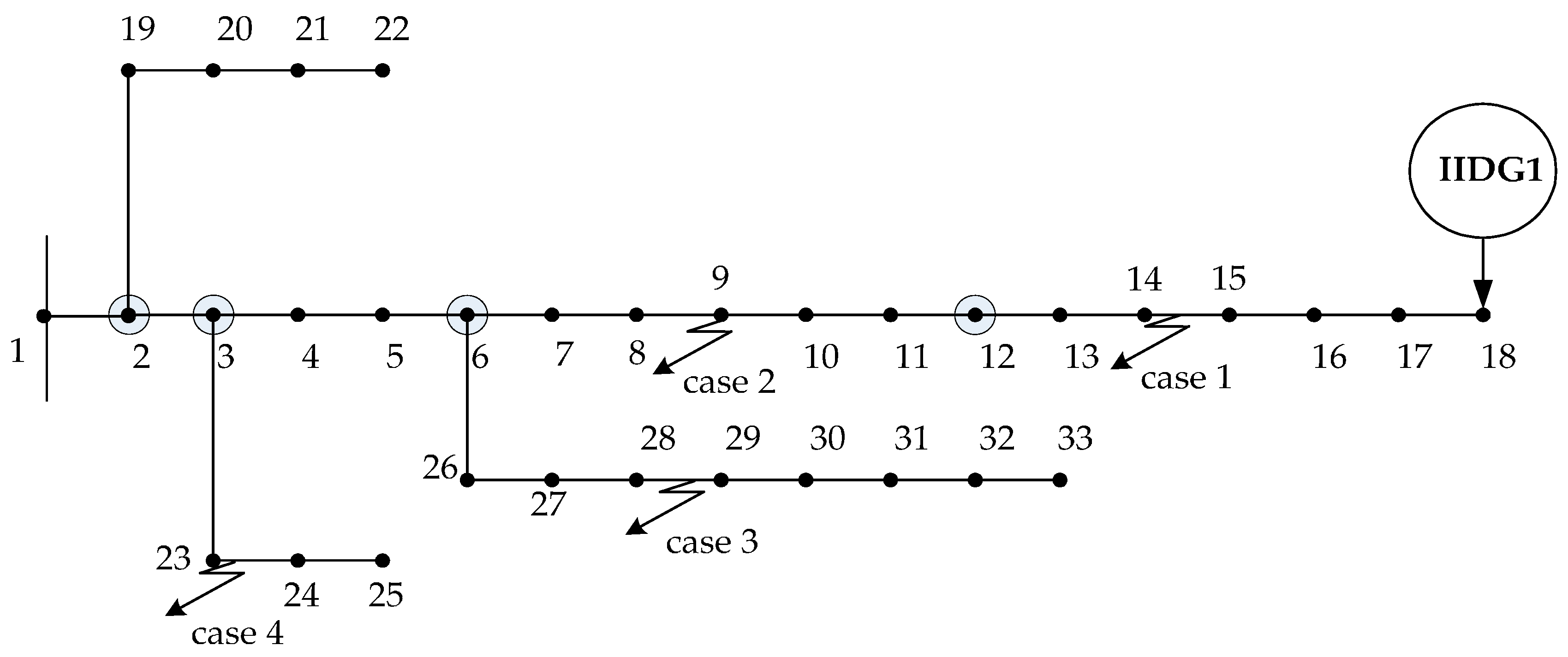
In this paper, the IEEE 33-node distribution system [26] is modified as shown in Figure 5 to verify the effectiveness and superiorities of proposed locating strategy. An IIDG of photovoltaic whose rated power is 0.4 MW is interfaced with node 18.

As shown with the circles in Figure 5, four power quality monitoring devices are located at node 2, node 3, node 6, and node 12, respectively. Real-time data of voltages and currents of the observation points are obtained by power system computer aided design (PSCAD)/electro-magnetic transient in direct current (EMTDC) time-domain simulation.

To guarantee the accurate obtainment of fundamental frequency voltage phasors and current phasors, time-frequency atomic transform (TFT) [27,28] is used to process the waveforms of voltages and currents. TFT has compact complex band-pass filter characteristic, ideal frequency characteristic, flexible and adjustable bandwidth in time-frequency domain.

To illustrate the effectiveness of the proposed strategy, the following four cases are used to give detailed descriptions.

(1)

Case 1: A-phase ground fault (A-G-F) occurs at branch 14–15, 40% away from node 14 with fault resistance of 10.0 ohm.

(2)

Case 2: AB-double-phase fault (AB-F) occurs at node 9 with fault resistance of 8.0 ohm.

(3)

Case 3: AB-double-phase ground fault (ABG-F) occurs at branch 28–29, 70% away from node 28 with fault resistance of 4.0 ohm.

(4)

Case 4: ABC-three-phase ground fault (ABC-G-F) occurs at branch 23–24, 20% away from node 23 with fault resistance of 1.0 ohm.

5.2. Locating Results of the Proposed Locating Strategy

According to the framework of the proposed locating strategy in Section 4, the results of the main procedures are illustrated with the following three subsections.

5.2.1. Cause Identification and Derivation of Candidate Area

Once a votage sag event is detected, the cause identification and derivation of candidate area set1 are the basis for further accurate locating. For the four cases, the corresponding results can be obtained as

Table 1. Results of cause identification and derivation of candidate area.

Case	Fault Type	Nodes in set1
Case 1	A-G	13, 14, 15, 16, 17, 18
Case 2	AB	7, 8, 9, 10, 11
Case 3	AB-G	26, 27, 28, 29, 30, 31, 32, 33
Case 4	ABC-G	23, 24, 25

. The results of fault type are judged by the rules in [25].

Concretely, in this paper, the direction of sag source relates to each branch is judged by the resistance sign-based method of [11]. Detailed results of the relative direction are shown in

Table 2. Results of upstream or downstream relationship judgment.

Branch	Case 1	Case 2	Case 3	Case 4
1–2	−	−	−	−
2–3	−	−	−	−
2–19	+	+	+	+
3–4	−	−	−	+
3–23	+	+	+	−
5–6	−	−	−	+
6–7	−	−	+	+
6–26	+	+	−	+
11–12	−	+	+	+
12–13	−	+	+	+

.

For each branch named as “c–d”, “c” and “d” are the head and end of the branch, respectively. In the table, “−“ means the sag source is on the downstream of the branch, namely the direction of the end “d”. On the contrary, “+” represents the sag source is on the upstream of the branch, namely the direction of the head “c”.

According to Table 2, it can be derived that the sag source is on the downstream of branch 2–3, downstream of branch 3–4, downstream of branch 6–7 and downstream of branch 12–13 for the four observation points in case 1, respectively. Therefore, the sag source of case 1 is located at downstream of node 12. That is, nodes in set1 of case 1 can be derived as 13, 14, 15, 16, 17, 18. Similarly, nodes in set1 for the other three cases can be derived.

5.2.2. Search the Nearest Node

As the first-step of the two-step optimization model, the objective function (3) is searched to find the ne-node in the candidate area set1. For the four cases, via the HPSO algorithm, the optimal solutions shown in

Table 3. Optimal solutions of f1 in searching the ne-node.

Case	f1	b	rf1/Ohm	set2
Case 1	0.0474	14	10.2310	branch 13–14, branch 14–15
Case 2	0.0058	9	7.9990	branch 8–9, branch 9–10
Case 3	0.2326	29	3.7396	branch 28–29, branch 29–30
Case 4	1.2404	23	1.1920	branch 23–24, branch 24–25

can be obtained.

From Table 3, it shows that the results of ne-node for the four cases are node 14, node 9, node 29 and node 23, respectively. Further, set2 which is consisted of all the branches connected with ne-node can be derived as the fifth column in Table 3.

To verify the correctness of above results in searching the ne-node, the following tests are carried out by taking case 1 as an example. Let b equals to 13, 14, 15, 16, 17 and 18, respectively, then the minimums of objective function f1 can be obtained as

Table 4. Optimal solutions of f1 when fault occurred at each node in set1 for Case 1.

f1	b	rf1/Ohm
0.1968	13	10.8272
0.0474	14	10.2310
0.0676	15	9.6569
0.1748	16	8.9685
0.4902	17	8.0061
0.5871	18	7.7902

with the only one variable of r_f1.

From Table 4, it can be found that 0.0474 is the minimum of all the values in the first column. That is, node 14 really is the ne-node for case 1.

5.2.3. Search the Precise Location

As the second-step of the two-step optimization model, the objective function of Formula (6) is sought to identify the faulted branch and precise fault location in set2. Via the HPSO algorithm, the optimal solutions shown in

Table 5. Optimal solutions of f2 in searching the precise location.

Case	f2	l	λ/%	rf2/Ohm
Case 1	0.0052	14–15	40.29	9.9980
Case 2	0.0058	8–9	100.0	7.9990
Case 3	0.0054	28–29	70.15	3.9994
Case 4	0.0046	23–24	19.76	1.0048

can be obtained.

To verify the correctness of above results of searching the precise location, the following tests are carried out by taking case 1 as an example. Let the faulted branch be 14–15 and 13–14, respectively. Then, the minimums of objective function f2 can be obtained as

Table 6. Optimal solutions of f2 when a fault occurred at each branch in set2 for Case 1.

f2	l	λ/%	rf2/Ohm
0.0052	14–15	40.29	9.9980
0.0474	13–14	100.0	10.2310

, which can illustrate that the results of Table 5 are correct.

According to Table 1 and Table 5, the locating results of the four voltage sag cases can be obtained as follows.

(1)

Case 1 is caused by A-phase ground fault, which occurs at branch 14–15, 40.29% away from node 14.

(2)

Case 2 is caused by AB-double-phase fault, which occurs at node 9.

(3)

Case 3 is caused by AB-double-phase ground fault, which occurs at branch 28–29, 70.15% away from node 28.

(4)

Case 4 is caused by ABC-three-phase ground fault, which occurs at branch 23–24, 19.76% away from node 23.

Compared above locating results with the actual situations of the four cases, the following conclusions can be obtained.

(1)

The faulted branches/node can be accurately located.

(2)

The errors of λ are 0.29%, 0, 0.15% and 0.24%, which are very small values.

Therefore, it can be summarized that the proposed strategy can realize accurate locating of voltage sag caused by short circuit fault in smart distribution network with IIDG.

5.3. Locating Performance Analyses

Further, to verify the superiorities of the proposed strategy in applicability and accuracy, tests and analyses are implemented in the following three perspectives:

(1)

The effect of IIDG capacity.

(2)

The effect of fault resistance.

(3)

The effect of the neutral ungrounded.

5.3.1. The Effect of IIDG Capacity on Locating Results

To test the effects of IIDG capacity on locating accuracy, the proposed strategy (Strategy 1 hereinafter), is used to locate case 1 with different capacities of IIDG. Detailed locating results can be obtained as

Table 7. Locating results of Strategy 1 with different capacities of IIDG.

IIDG Capacity/MW	ne-node	l	λ/%	rf2/Ohm
0.2	14	14–15	40.25	9.9945
0.4	14	14–15	40.29	9.9980
0.6	14	14–15	40.10	10.0059
0.8	14	14–15	39.82	9.9996

.

From Table 7, it can be seen that:

(1)

All results of the faulted branch are correctly located as branch 14–15.

(2)

The errors of λ are 0. 25%, 0.29%, 0.10% and 0.18%, which are very small values with no significant fluctuation.

By the way, the locating strategy (Strategy 2 hereinafter) of [7], which has good locating performance for traditional radial distribution network with only one power supply, is used to locate case 1 with different capacities of IIDG. Concrete locating results are as shown in

Table 8. Locating results of Strategy 2 with different capacities of IIDG.

IIDG Capacity/MW	ne-node	l	λ/%	rf2/Ohm
0.2	14	13–14	89.32	10.4375
0.4	14	13–14	77.73	10.4040
0.6	13	13–14	17.84	11.0422
0.8	13	13–14	3.30	11.0516

.

While from Table 8, it can be seen that:

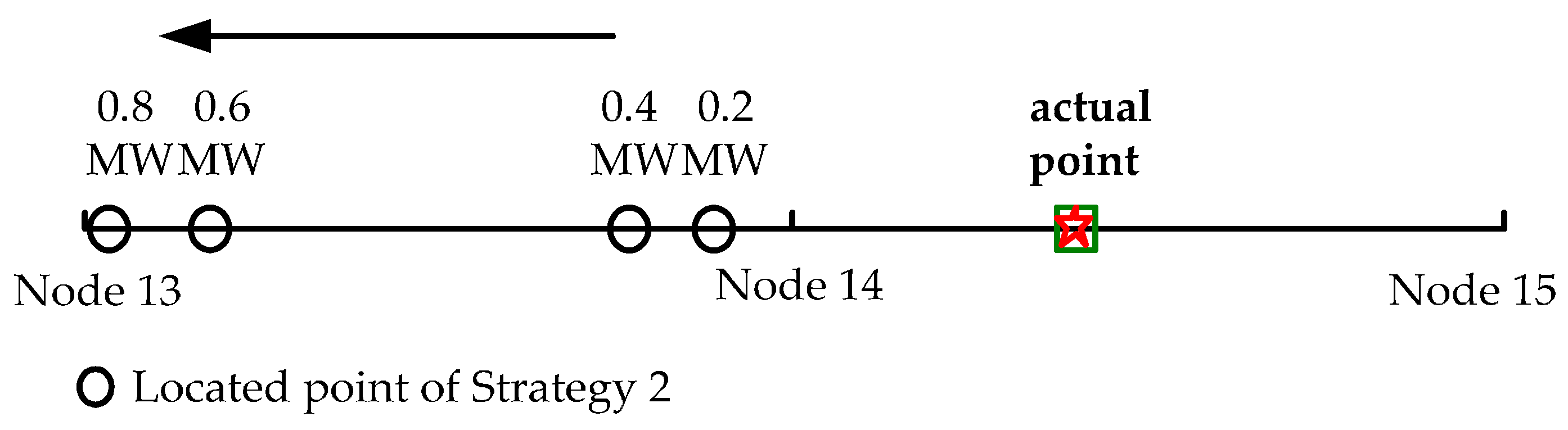
(1)

When IIDG capacities are 0.2 MW, 0.4 MW, 0.6 MW and 0.8 MW, respectively, results of the faulted branch are mistakenly located as branch 13–14.

(2)

With the increase of IIDG capacity, the located sag source is getting closer to node 13 as shown in Figure 6. That is, the locating error is becoming larger.

To sum up, it shows that the proposed strategy is feasible to smart distribution network with IIDG. With the increase of IIDG capacity, the advantage in locating accuracy will be more prominent.

5.3.2. The Effect of Fault Resistance on Locating Results

Moreover, to test the effect of fault resistance on locating results, Strategy 1 is used to locate case 1 with different values of fault resistance. The capacity of IIDG is set as 0.4 MW. Detailed locating results can be obtained as

Table 9. Locating results of Strategy 1 with different fault resistances.

Fault Resistance/Ohm	ne-node	l	λ/%	rf2/Ohm
2.5	14	14–15	39.70	2.4995
5	14	14–15	39.91	4.9960
10	14	14–15	40.29	9.9980
20	14	14–15	40.15	19.9994
40	14	14–15	40.29	40.0177

.

From Table 9, it can be seen that:

(1)

All results of the faulted branch are correctly located as branch 14–15.

(2)

The errors of λ are 0.30%, 0.09%, 0.29%, 0.15% and 0.29%, which are very small values with no significant fluctuation.

Further, Strategy 2 is used to locate case 1 with different values of fault resistance as well. Concrete locating results are as shown in

Table 10. Locating results of Strategy 2 with different fault resistances.

Fault Resistance/Ohm	ne-node	l	λ/%	rf2/Ohm
2.5	14	14–15	0.0	2.8862
5	14	13–14	94.89	5.3920
10	14	13–14	77.73	10.4040
20	13	13–14	0.52	20.9269
40	13	12–13	43.85	41.6195

.

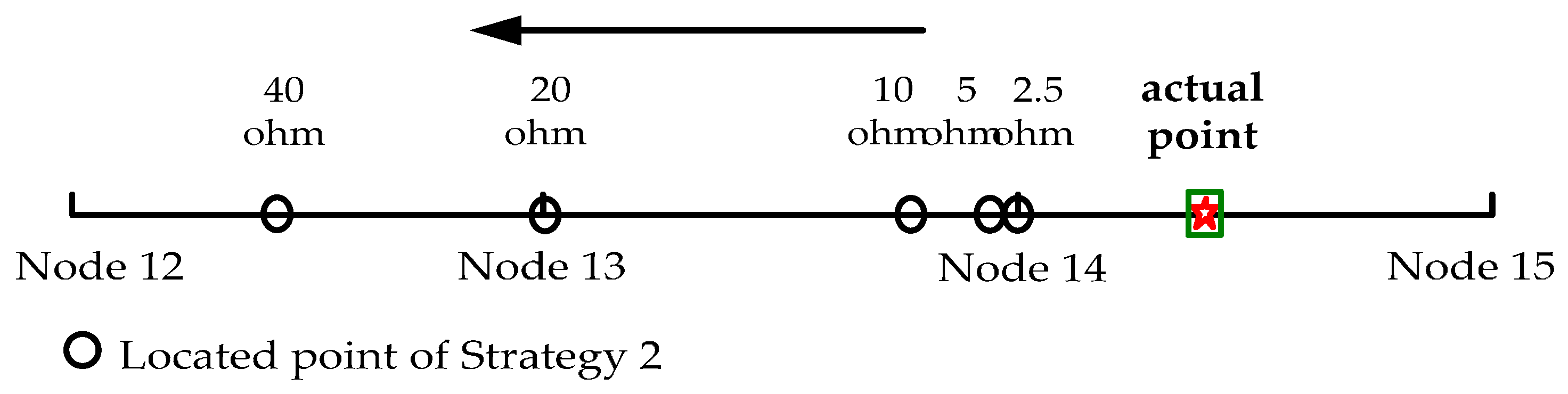
While from Table 10, it can be seen that:

(1)

When actual fault resistance is 5 ohm/10 ohm/20 ohm, the faulted branch is mistakenly located as branch 13–14. And, when actual fault resistance is 40 ohm, the faulted branch is mistakenly located as branch 12–13.

(2)

With the increase of actual fault resistance, the located sag source is getting far away from the actual location as shown in Figure 7. That is, the locating error is becoming larger.

To sum up, it shows that the proposed strategy has higher locating accuracy by optimizing fault resistance in the two-step locating model. With the increase of fault resistance, the advantage in locating accuracy will be more prominent.

5.3.3. Locating Results of the Proposed Strategy under the Neutral Ungrounded

Above tests are carried out under the neutral grounded. Ulteriorly, tests to analyze the effect of the neutral ungrounded on locating accuracy of the proposed strategy are carried out. The modified IEEE 33-node system is set as the neutral ungrounded. And, case 1 with different values of fault resistance is located via the proposed strategy. The capacity of IIDG is set as 0.4 MW. Concrete locating results can be obtained as

Table 11. Locating results of Strategy for Case 1 under the neutral ungrounded.

Fault Resistance/Ohm	ne-node	l	λ/%	rf2/Ohm
2.5	14	14–15	40.13	2.4998
5	14	14–15	39.85	5.0008
10	14	14–15	40.18	9.9982
20	14	14–15	40.12	19.9985
40	14	14–15	40.21	40.0073

.

From Table 11, it can be seen that:

(1)

All results of the faulted branch are correctly located as branch 14–15.

(2)

The errors of λ are 0.13%, 0.15%, 0.18%, 0.12% and 0.21%, which are very small values with no significant fluctuation. Compared with the results in Table 9, which is obtained by the proposed strategy under the neutral grounded, the locating accuracy has no obvious difference.

Above results show that the proposed strategy can also realize accurate locating of voltage sag caused by short circuit fault in smart distribution network under the neutral ungrounded. That is, the applicability and accuracy of the proposed strategy are insensitive to the neutral grounding mode.

5.4. Locating Results of the Proposed Strategy in the Modified IEEE 69-Node Benchmark

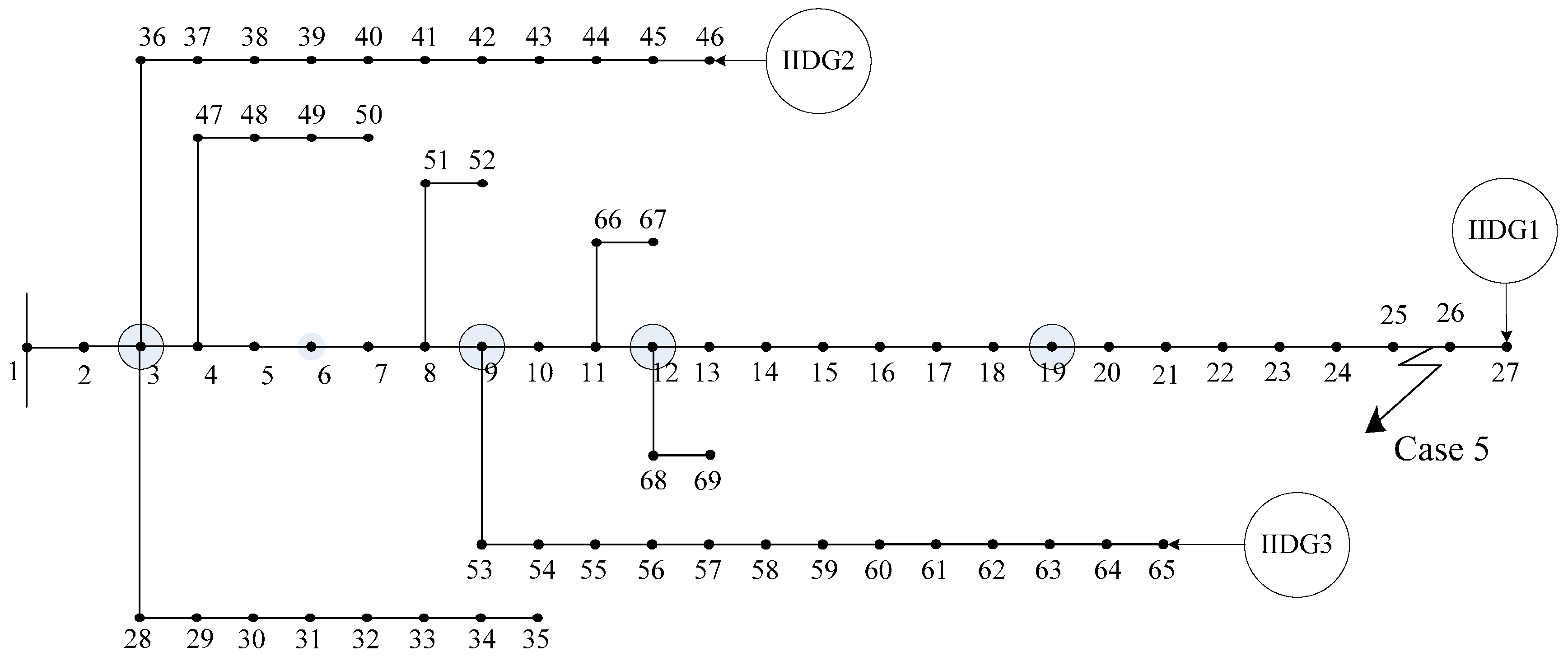
Moreover, to verify the effectiveness and superiorities of proposed locating strategy in larger scale benchmark with more IIDGs, the IEEE 69-node distribution benchmark [29] is modified by adding 3 IIDGs. As shown in Figure 8, IIDG1, IIDG2 and IIDG 3, whose rated power are all 0.4 MW, are interfaced with node 27, node 46 and node 65, respectively. Four power quality monitoring devices remarked by the circles are located at node 3, node 9, node 12 and node 19, respectively.

For different fault scenarios in the modified 69-node distribution benchmark, the proposed strategy accurately located the fault locations.

Limited by space, the following Case 5 is selected as the example to give illustration of the results of main locating procedures and carry out comparisons. Case 5: A-phase ground fault (A-G-F) occurs at branch 25–26, 70% away from node 25 with fault resistance of 5.0 Ohm.

5.4.1. Results of Main Procedures for Locating Case 5

The results of main procedures for locating case 5 are as follows.

(1)

Case 5 is identified caused by A-phase ground fault. And the candidata area set1 is determined as the downstream of branch 19–20. Therefore, set1 contains node 20, node 21, node 22, node 23, node 24, node 25, node 26, node 27.

(2)

By solving the first-step of the two-step optimization model in set1, the ne-node of case 5 is identifed as node 26, whicn can be verifed by the results shown in

Table 12. Optimal solutions of f1 when fault occurred at each node in set1 for Case 5.

f1	b	rf1/Ohm
0.5562	20	6.8206
0.2201	21	6.4095
0.2182	22	6.3994
0.1945	23	6.2539
0.1439	24	5.9251
0.0346	25	5.1982
0.0185	26	4.9136
0.0434	27	4.7619

. In the frist column of the table, it can be seen that 0.0185 is the minimum. Therefore, the set2 can be determined as branch 25–26 and branch 26–27.

(3)

By solving the second-step of the two-step optimization model in set2, the fault point is located at branch 25–26, 70.12% away from node 25, which can be verifed by the results shown in

Table 13. Optimal solutions of f2 when fault occurred at each branch in set2 for Case 5.

f2	l	λ/%	rf2/Ohm
0.0056	25–26	70.12	5.0013
0.0185	26–27	100.0	4.9136

. In the frist column of the table, it can be seen that 0.0056 is the minimum.

Therefore, the locating result of case 5 is that it is caused by A-phase ground fault, which occurs at branch 25–26, 70.12% away from node 25. It can be seen that the faulted branch is accurately located and the error of λ is merely 0.12% compared with the actual situation. This shows that the proposed Strategy 1 can realize accurate locating of voltage sag caused by short-circuit fault in smart distribution network with multiple IIDGs.

5.4.2. The Effect of IIDG Capacity on Locating Results for Case 5

To test the effect of IIDG capacity on locating accuracy in the modified IEEE 69-bus benchmark, the proposed Strategy 1 and Strategy 2 are used to locate case 5 with different capacities of IIDG1. Detailed locating results can be obtained as

Table 14. Locating results of Strategy 1 with different capacities of IIDG1 for Case 5.

IIDG1 Capacity/MW	ne-node	l	λ/%	rf2/Ohm
0.2	26	25–26	70.25	4.9996
0.4	26	25–26	70.12	5.0013
0.6	26	25–26	70.31	4.9991
0.8	26	25–26	70.25	4.9988

and

Table 15. Locating results of Strategy 2 with different capacities of IIDG1 for Case 5.

IIDG1 Capacity/MW	ne-node	l	λ/%	rf2/Ohm
0.2	25	24–25	99.23	5.2287
0.4	25	24–25	97.57	5.2268
0.6	24	24–25	2.82	5.9274
0.8	24	24–25	1.18	5.8991

.

From Table 14 and Table 15, it can be seen that:

(1)

All the results of the faulted branch obtained by the proposed Strategy 1 are correctly located as branch 25–26. And, the errors of λ are 0.25%, 0.12%, 0.31% and 0.25%, which are very small values with no significant fluctuation.

(2)

While when IIDG1 capacities are 0.2 MW, 0.4 MW, 0.6 MW and 0.8 MW, respectively, the results of the faulted branch obtained by Strategy 2 are mistakenly located as branch 24–25. Further, from the results in Table 15, it can be seen that the located sag source is getting closer to node 24 with the increase of the capacity of IIDG1. That is, the locating error is becoming larger.

To sum up, for smart distribution network with multiple IIDGs, the advantage of the proposed strategy in locating accuracy will be more prominent with the increase of IIDG capacity.

5.4.3. The Effect of Fault Resistance on Locating Results for Case 5

Moreover, to test the effect of fault resistance on locating results, the proposed Strategy 1 and Strategy 2 are used to locate Case 5 with different values of fault resistance. The capacity of IIDG1 is set as 0.2 MW. Detailed locating results can be obtained as

Table 16. Locating results of Strategy 1 with different fault resistances for Case 5.

Fault Resistance/Ohm	ne-node	l	λ/%	rf2/Ohm
2.5	26	25–26	69.79	2.5005
5	26	25–26	70.12	5.0013
10	26	25–26	70.23	9.9995
20	26	25–26	70.15	20.0002

and

Table 17. Locating results of Strategy 2 with different fault resistances for Case 5.

Fault Resistance/Ohm	ne-node	l	λ/%	rf2/Ohm
2.5	25	25–26	13.69	2.6871
5	25	24–25	99.96	5.2235
10	24	24–25	3.03	10.9714
20	23	23–24	3.91	21.2674

.

From Table 16 and Table 17, it can be seen that:

(1)

All the results of the faulted branch obtained by the proposed Strategy 1 are correctly located as branch 25–26. And, the errors of λ are 0.21%, 0.12%, 0.23%, 0.15%, which are very small values with no significant fluctuation.

(2)

While when the values of actual fault resistance are 5 ohm, 10 ohm and 20 ohm, the results of the faulted branch obtained by Strategy 2 are mistakenly located as branch 24–25, branch 24–25 and branch 23–24, respectively. Further, from the results in Table 17, it can be seen that the located sag source is getting closer to node 23 with the increase of fault resistance. That is, the locating error is becoming larger.

To sum up, for smart distribution network with multiple IIDGs, the advantage of the proposed strategy in locating accuracy will be more prominent with the increase of fault resistance.

5.5. The Effects of Measurement and Model Errors on Locating Accuracy of the Proposed Strategy

Moreover, the effects of measurement and model errors on locating accuracy of the proposed strategy are analyzed. In detail, the following two groups of tests are carried out in Case 1.

5.5.1. The Effect of Measurement Error on Locating Accuracy

Suppose all the magnitudes of the observed voltages and currents are 100.5%, 101%, 102% times the actual values, respectively. Without these information, the proposed strategy is implemented to locate Case 1. Specific locating results as shown in

Table 18. Locating results of Strategy 1 with different measurement errors for Case 1.

Measurement Error	l	λ/%	rf2/Ohm
0%	14–15	40.29	9.9980
0.5%	14–15	35.85	10.2048
1%	14–15	32.75	10.3924
2%	14–15	20.12	10.8433

can be obtained.

From Table 18, it can be seen that:

(1)

With the increase of measurement error, the locating error of the proposed Strategy 1 will be increased accordingly. Concretely, the results of the faulted branch under measurement errors of 0.5%, 1% and 2% are correct, while the errors of λ are 4.85%, 7.25% and 19.78%.

(2)

For measurement error within 1%, the locating error of the proposed strategy shows no significant increase.

With the widely applications of new signal processing algorithms and monitoring devices with better performances, the measurement error can be reduced to lower the side influence on the locating accuracy of the proposed strategy.

5.5.2. The Effect of Load Model Error on Locating Accuracy

As the loads can vary at different times, the load model error is selected as the example to test the effects of model error. Suppose the power of all the loads are 102.5%, 105% and 110% times of the rated values, respectively. Without these information, the proposed strategy is implemented to locate case 1. Specific locating results as shown in

Table 19. Locating results of Strategy 1 with different errors of loads model for Case 1.

Load Model Error	l	λ/%	rf2/Ohm
0	14–15	40.29	9.9980
2.5%	14–15	44.86	10.0450
5%	14–15	48.53	10.0820
10%	14–15	57.31	10.1737

can be obtained.

From Table 18, it can be seen that:

(1)

With the increase of load model error, the locating error of the proposed Strategy 1 will be increased accordingly. Concretely, the results of the faulted branch under load model errors of 2.5%, 5% and 10% are correct, while the errors of λ are 4.86%, 8.53% and 17.31%.

(2)

For load model error within 5%, the locating error of the proposed strategy shows no significant increase.

With the installations of more and more intelligent measurement units in the smart distribution network, it offers the possibility of more frequent update of the information of loads, which can reduce the error of load model. That is, the side influence of load model error on the locating accuracy of the proposed strategy can be lowered.

6. Discussion

The results obtained with two different scale benchmarks show that the proposed strategy has good feasibility and accuracy performance for locating voltage sag sources in smart distribution networks. It has pointed out that:

(1)

By considering the effects of IIDGs in short-circuit calculation, the proposed strategy has better feasibility. With the wide integration of IIDGs, smart distribution networks have been transformed into active complex networks with two or more power supplies. As the result, the distribution of short-circuit voltages and currents in smart distribution networks is different from that of the traditional distribution networks. Therefore, the methods based on the characteristics of traditional distribution networks are no longer suitable for smart distribution networks and have non-ideal accuracy.

(2)

By re-optimizing fault resistance in the second-step of the proposed two-step optimization model, the proposed strategy has better locating accuracy by eliminating the estimation error of fault resistance. For the short-circuit fault occurs at a branch rather than a node, the faulted node is not the accurate fault location. Therefore, there exists a difference between the optimal rf1 and the actual fault resistance. This error affects the precision of short-circuit calculation and further results in negative impacts on locating accuracy.

(3)

As the short-circuit calculation method is universal with different zero sequence networks for a system under different neutral grounding modes, the proposed strategy is insensitive to the neutral grounding mode.

(4)

(4) Furthermore, as the results in Section 5.5 show, the measurement and model errors can lead to side influences on locating accuracy of the proposed strategy. In future, on the one hand, new signal processing algorithms and monitoring devices with better performances can be introduced to lower the side influences. On the other hand, in-depth study is to be done to improve the robustness of the proposed strategy for the measurement and model errors.

7. Conclusions

With the aid of PQMS and DAS, a novel strategy for accurate locating of voltage sag sources in smart distribution networks with IIDGs is proposed. Concretely, based on inverse theory, a two-step optimization model is proposed for complex active distribution network. Further, on the one hand, by considering the effects of IIDGs in short-circuit calculation, the feasibility of the proposed strategy is guaranteed. On the other hand, by optimizing fault resistance twice, the estimation error of fault resistance can be eliminated. Therefore, the locating accuracy of the proposed strategy is improved.

Cases studies via a modified IEEE 33-node benchmark and a modified IEEE 69-node benchmark verified the effectiveness of the strategy. Moreover, locating results show that the superiority of the proposed strategy in locating accuracy will be more prominent with the increase of IIDG capacity and/or the increase of fault resistance.

The proposed strategy shows good feasibility and locating accuracy performance for smart distribution networks with single IIDG or multiple IIDGs. It is insensitive to IIDG capacity, fault resistance and the neutral grounding mode.