1. Introduction
Due to their high energy consumption and the high demand for installation of these devices in the buildings, nowadays different controllers are applied in heating, ventilating and air-conditioning systems (HVACs) to improve the system performance. The most significant considerations when designing HVAC systems are the indoor thermal conditions and energy efficiency [
1]. The complicated features of HVAC systems make mathematical modelling of systems very difficult or sometimes impossible [
1]. Therefore, the design of proper controllers for HVAC systems has become a great challenge [
2,
3]. As the HVAC systems use high amounts of energy, even small improvements in the system operational efficiency can result in significant energy savings [
4]. Hence, many studies have been done in the control of HVAC and A/C systems and the optimization area.
Providing thermal comfort is the main and most important purpose of designing the HVAC, and A/C systems in buildings. Therefore, advanced control methods are needed to consider the MIMO, nonlinearity, coupling effect of the parameters and complex features of the system, while at the same time considering the occupant’s thermal comfort demand and the system’s energy efficiency. Hence, MIMO, nonlinear, intelligent and robust controllers are desired to achieve the mentioned aims simultaneously. Accordingly, the intelligent base soft computing control scenario is required to consider the nonlinearity and MIMO structure of the system.
As one of the most important concerns of control engineers is to mimic reality as close as possible and also for the designed system to be practically applicable, designing advance control techniques by taking into account the characteristics of the system is required. As the purpose of this work is to control a direct expansion air conditioning (DX A/C) system, the MIMO, coupled parameters, and nonlinearity structure of the system should be considered in any control algorithm.
As the structures of HVAC systems are complex and uncertain, the application of nonlinear control methods has limitations. The most important reasons among others are the complex mathematical analysis, stability analysis and dependence on a whole set of states [
5]. The air-handling unit (AHU) was controlled separately by gain scheduling and feedback linearization methods [
6]. Both methods were applied on a non-linear MIMO dynamic model of an AHU in which the air flow rates and cold water are used for achieving to the desired indoor temperature and humidity. Controlling the system by using the feedback linearization method, the tracking objectives of temperature and humidity ratio are very quick, but the results show more overshoots. By applying the gain scheduling controller on an AHU, less energy consumption was achieved. In order to track the objectives, less variation of air and cold water flow rates are required. In contrast, by using a gain scheduling method, the identification of linear regions and design of switching logic between regions is essential. PID controllers are used as switching logic between regions and their manual tuning can be quite cumbersome. A non-linear adaptive back-stepping control algorithm was used to control multi-variable nonlinear mathematical model HVAC systems [
7]. The Lyapunov stability is used in this method. Energy management of the system is achieved by using this energy efficient controller, therefore, this control method has been utilized in the field of intelligent building energy saving. The disadvantages of this method are the need for a bilinear observer, and the difficulty in finding Lyapunov stability. A back-stepping controller on the feedback linearized model of the single-zone VAV HVAC & R system was applied by Qi [
8]. A bilinear model was used to describe the temperature and humidity dynamics. The heat and moisture loads were considered as measurable disturbances. The back-stepping controller was used on the feedback linearized model in order to design a stable observer for non-measurable disturbances backed by simulation results to attain the optimal energy consumption. The simulation results of the closed-loop system indicate good and fast tracking, offset-free and smooth response with high disturbance decoupling and optimal energy consumption properties in the presence of time-varying loads. Due to the difficulty in finding a Lyapunov function, all state variables must be measurable; otherwise, the need for a non-linear observer is one of the shortcomings of this method. In other words, the complex mathematic analysis, and the need to design the linearization controller and decouple the model to find some required parameters, using others method to transform the linearized model into a non-linear form are the main disadvantages of this control design. A Non-Linear Optimal Controller for HVAC systems was designed based on input/output feedback linearization, a MATLAB/Simulink response optimizer and non-linear programming by Dong [
9]. By designing the non-linear optimal controller, energy savings are obtained. The main contribution of this control method is the development of sustainable and energy efficient buildings. Additional parameters are however required in this method, which makes the integration in real HVAC systems difficult and impractical. Hence, the application of non-linear control methods like feedback linearization, gain scheduling, and back-stepping controllers presents some disadvantages such as overshoots, identification of linear regions, design of switching logic between regions, difficulty in finding a Lyapunov function, linearization and decoupling the model to find some required parameters, by using another method to transfer the model to the non-linear form.
HVAC and A/C systems are basically MIMO systems. Nevertheless, sometimes for making the control design easy, they are considered as SISO systems when designing a controller [
3]. It is clear that the performance of MIMO control strategies is inherently better than conventional SISO control strategies. In addition, due to the coupling effect between parameters, especially in the DX A/C structure, MIMO control strategies are required to consider the coupling effects of variables. Online auto-tuned Takagi–Sugeno Fuzzy Forward control is used on the non-linear model of HVAC systems by using predicted mean vote index (PMV) as an objective instead of temperature and relative humidity. This method is able to solve the coupling effect of temperature and humidity. The accuracy and efficiency by optimizing between the temperature and relative humidity are achieved by using PMV as a reference. Nonetheless, the implementation of fuzzy logic control requires comprehensive knowledge of the plant operation and its different states. The GPC method was applied for tuning the PID controller parameters by Xu et al. [
10], as well as Xu and Li [
11] which used the GPC method to decouple a HVAC & R system together with parameter identification. In comparison to the coupled system, this method requires less computation.
In the HVAC area MIMO control strategies are mostly applied to the linearized model of the system around the operating point. This means that the controller works in a limited range. The MIMO Linear Quadratic Gaussian (LQG) control method was applied on a DX A/C system by Qi [
6]. The linearized model of the DX A/C system is used at the system’s operating point, meaning that the designed controller is not suitable for non-linear conditions and it only works and is stable around that operating point. The controller is not implemented for a wider operating range. The controller results are in the range of 24 °C for temperature and 50% for humidity, and the controller does not have the ability to decrease the temperature from more than 25 °C and humidity from more than 60%. A linear predictive control concept for a solar powered HVAC system was used by Ferhatbegovíc et al. [
12]. Dynamic models of the HVAC components were used for designing the controller and validated by carried out measurements on a real HVAC system. By using weather forecast information, the MPC performance indicates excellent performance, even when the incorrect information is provided by a weather forecast. The receding horizon strategy of the MPC concept strictly accounts for such cases where the predicted information is not correct. Thus, a non-linear model predictive controller is required.
As the purpose of this study is to control a DX A/C system, the problem when designing a suitable controller is how to hold the features of the system unchanged which have a MIMO structure, the coupling effect between parameters and non-linearity by designing a simple structure and easy implementation controller. In other words, which method is suitable for designing the controller in which the structure of the system is considered as non-linear MIMO with coupling effects and at the same time this controller should be practically applicable. In order to solve this problem, the chosen method for designing the controller is based on a Fuzzy Cognitive Map. Due to the specific structure of this method, the MIMO structure and coupling effect can be consider as a graph structure network by choosing the inputs and outputs of the system as nodes for the graph and the coupling effect between parameters can be shown and considered as a relationship between concepts and considering their effects on each other. The value of the parameters are applied on the non-linear model of the system and the non-linearity is also considered by this structure.
2. Methodology
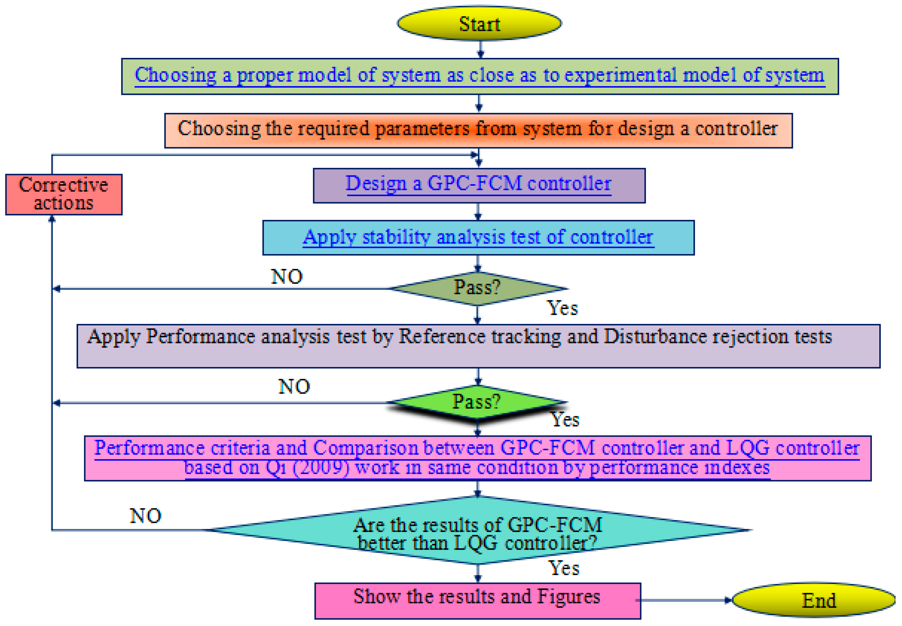
The methodology flow chart of this work is illustrated in
Figure 1. This flow chart is based on the methodology of this work in order to design a proper controller for the DX A/C system. In addition, it includes a stability analysis test of the proposed controller and its performance analysis by set point tracking, and disturbance rejection. Finally, a comparison between the mentioned controller and the Qi [
8] work has been done under the same conditions for both controllers.
In order to control the DX A/C system, a control algorithm is required by considering the MIMO, non-linearity and coupling effect features of the system. Due to the structure of the GPC-FCM method for controlling the DX A/C system, the important characteristics of the system are considered. This intelligent MIMO nonlinear control algorithm is the main contribution of this study. By applying this control algorithm, the non-linear controller is designed without involving a difficult mathematic analysis for deriving the control law process. Better performance and energy savings are obtained by using the proposed controller in comparison with the previous applied controller on the same DX A/C system.
2.1. Choosing a Proper Model of the System
The model of the DX A/C system in this research was adopted from Qi’s [
8] work. In order to mimic the conditions as closely as possible to the real conditions, the model offered by Qi [
8] is chosen as an experimental model of the system, due to the experimental validation of the simulation model. The equation which was offered as an experimental model of the system are accurate enough to mimic the real conditions. This model is experimentally validated and established as a multivariable control-oriented modeling of a direct expansion air conditioning system. In other words, this model which is explained completely and comprehensively in the following sections, is almost practically same as the experimental behavior of the DX A/C system [
6,
8,
13,
14,
15].
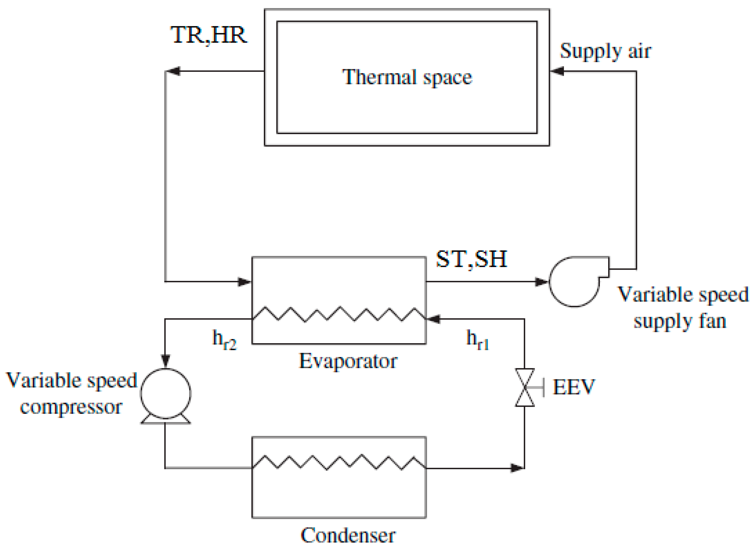
The construction of DX A/C system is divided into two parts: the air distribution part (air-conditioned room, supply fan, and ductwork) and the refrigeration part (evaporator, compressor, condenser, expansion valve, receiver, and oil separator) [
16,
17]. The desired set points for the air-conditioned room are provided by changing the speed of the compressor and the flow rate of the fan.
Figure 2 shows the structure of a direct expansion air conditioning system with a variable speed compressor and supply fan. The structure of the DX A/C system and the dynamic mathematical model of the system is based on several works [
6,
8,
13,
15,
18]. The required equations of the system which are achieved by using the principle of energy balance are described as follows [
6,
8,
13,
14,
15,
16,
17,
19]:
Table 1 lists the DX A/C system’s parameters and their descriptions.
Table 2 lists the numerical values and operating point of the DX A/C system based on [
8].
With the purpose of designing the MIMO non-linear controller of the DX A/C system, all the above differential equations should be rewritten in the state-space format. Consequently, the state-space form of the DX A/C system model can be expressed in the following compact format [
6,
8,
13]:
is the state vector.
is the control input and
is the disturbance.
g1,
g2 are the functions described as follows:
2.2. Choosing the Required Parameters from the System for Designing a Controller
Based on the control scenario algorithm for controlling the DX A/C system, the essential parameters selected as concepts of the controller are the following:
The air-conditioned room temperature (outputs).
The air-conditioned room humidity (outputs).
Supplied temperature (inputs).
Supplied humidity (inputs).
Speed of compressor (control signals).
Supply fan’s flow rate (control signals).
2.3. Designing the Proposed Controller
A DX A/C system is a non-linear, inherently complex and MIMO system with coupling effects on supplied temperature and supplied humidity. It needs to control the air humidity and air temperature of the air-conditioned room at the same time by taking into account the coupling effect on exiting air humidity and temperature from the evaporator (supply air humidity and temperature), while also decreasing the energy usage of the system. Hence, a fast, robust, closed-loop and inherently simple control algorithm is required to achieve the desired temperature and humidity.
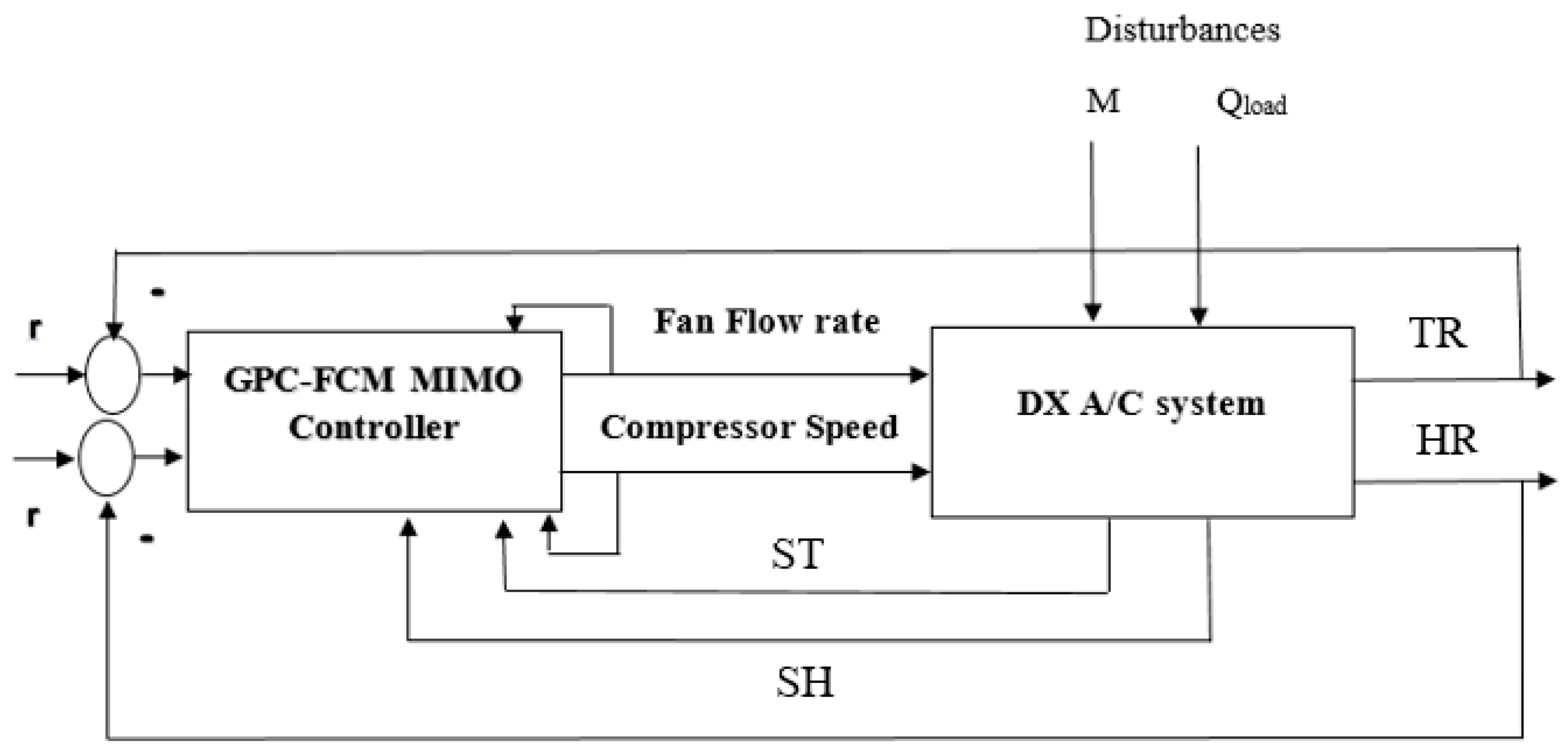
The chosen method for controlling the DX A/C system is a hybrid Generalized Predictive Control-Fuzzy Cognitive Map (GPC-FCM) controller. The core controller in this design is based on the FCM structure. The inputs and outputs of the system could be easily defined by the FCM method as nodes based on the control requirements of the system and the expected system performance scenario. In addition, the control variables are considered as effective parameters of the system. Since by changing the fan’s flow rate and the speed of the compressor, control of the system is achieved, then these two parameters should be considered in the control design. Thus, the MIMO approach could be used without the linearization of the system. The other positive point of this structure is the causal relationship between the concepts in which the coupling effect between concepts could be considered as two side relationship of coupled parameters.
In order to assign suitable weights between the nodes of the FCM structure, the GPC method is used to find the minimum required values for the fan’s flow rate and speed of the compressor. By combination of these two methods as a core controller and weight assigning controller, the hybrid method based on FCM and GPC methods is established.
Figure 3 shows the block diagram of the closed loop system.
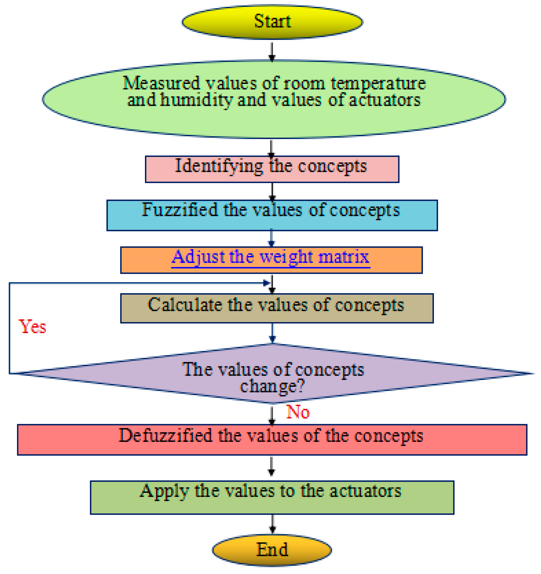
The FCM control algorithm step by step is as follows:
- (1)
Identification of the correct and required concepts from the system, like inputs and outputs and any affecting parameters on the system as concepts and assigning the initial weights between the concepts based on GPC method.
- (2)
Fuzzification of the concept values [
20,
21] by transformation mechanism.
- (3)
The weight matrix are adjusted by the differences within the concept values and their desired values [
22,
23].
- (4)
The next step values of the controller are calculated by Equations (12) and (13).
- (5)
The required values of the concepts are defuzzified and applied to the actuators.
Figure 4 shows the control design flow chart.
2.3.1. Measuring the Values of the Room Temperature and Humidity and Values of the Actuators
The values of the air-conditioned room and air-conditioned humidity are calculated based on Equations (1) and (2). Also, the values of the supply air temperature and supply humidity are calculated based on Equations (4) and (5). The values of actuators are calculated based on the FCM mathematics which are explained in the section on calculation of the concept values. All of the calculated values are assumed to be the same as the measured ones.
2.3.2. Identifying the Concepts
In this design, six important parameters from the system are identified for designing the controller. The concepts for DX A/C model should be described as follows:
A1: Temperature of the room (TR),
A2: Humidity of the room (HR),
A3: Supply temperature (ST),
A4: Supply humidity (SH),
A5: Compressor speed (CS), and
A6: Flow rate of fan (FF) [
24].
2.3.3. Fuzzification of the Values of the Concepts
Based on the FCM’s structure, the real measured values of the concepts should be transformed to the interval [0, 1]. By using the transformation mechanism, the real values of concepts are shifted to their fuzzy values. The selected transformation mechanism is [
24]:
where
sit is the measured value of the
ith state at time
t,
ai is min,
mi is average and
bi is max.
2.3.4. Linkage among the Concepts
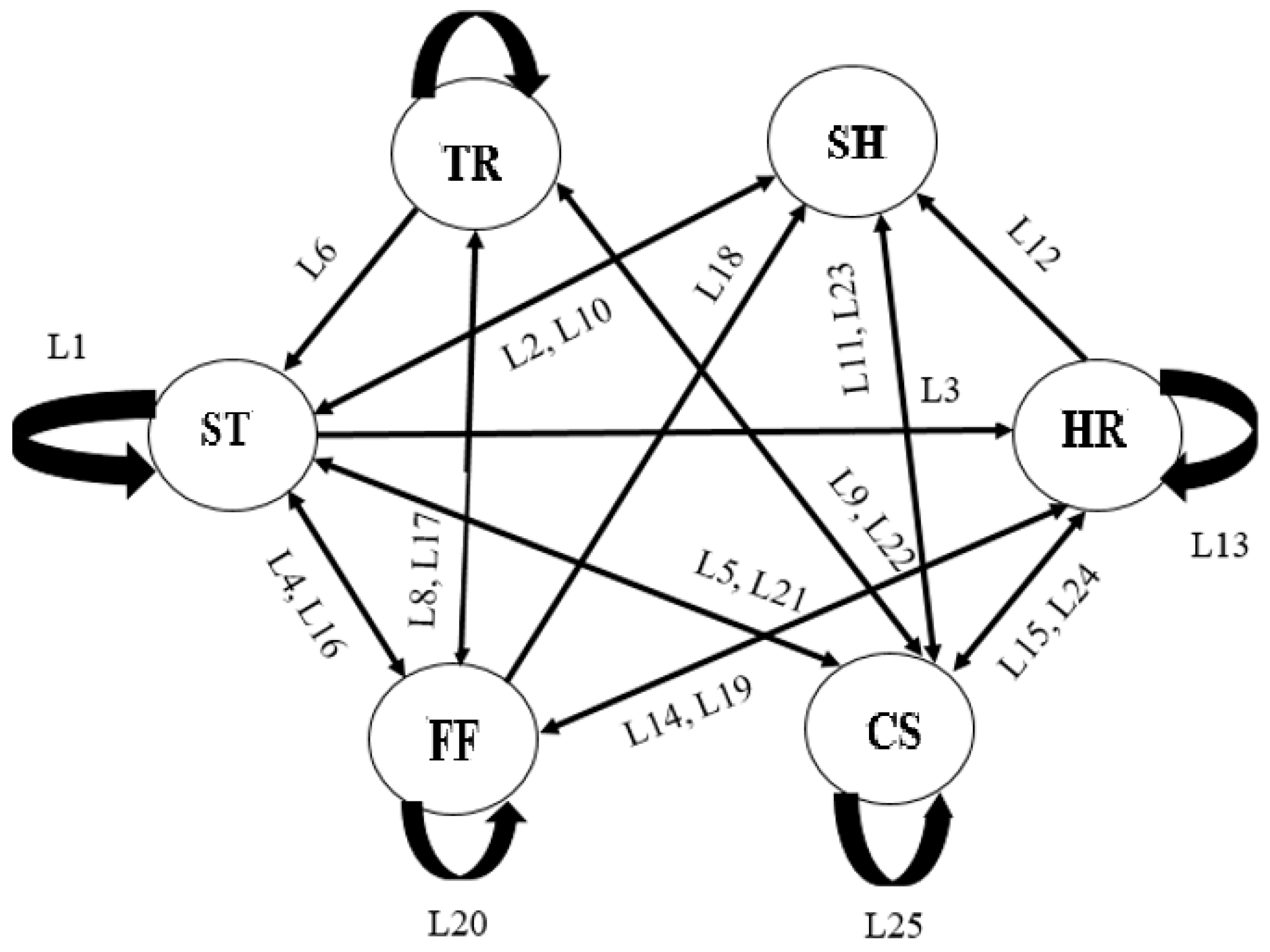
The linkages between concepts are explained as follows:
- Linkage 1 (L1):
The supply temperature (ST) has negative connection to supply temperature (ST).
- Linkage 2 (L2):
The supply temperature (ST) has positive connection to supply humidity (SH).
- Linkage 4 (L4):
The supply temperature (ST) has positive connection to the flow rate of fan (FF).
- Linkage 5 (L5):
The supply temperature (ST) has positive connection to compressor speed (CS).
- Linkage 7 (L7):
The temperature of the room (TR) has negative connection to the temperature of the room (TR).
- Linkage 8 (L8):
The temperature of the room (TR) has negative connection to the flow rate of fan (FF).
- Linkage 9 (L9):
The temperature of the room (TR) has positive connection to speed of compressor (CS).
- Linkage 10 (L10):
The supply humidity (SH) has positive connection to supply humidity (SH).
- Linkage 11 (L11):
The supply humidity (SH) has positive connection to compressor speed (CS).
- Linkage 12 (L12):
The humidity of the room (HR) has positive effect to supply humidity (SH).
- Linkage 13 (L13):
The humidity of the room (HR) has negative connection to humidity of the room (HR).
- Linkage 14 (L14):
The humidity of the room (HR) has negative connection to the flow rate of fan (FF).
- Linkage 15 (L15):
The humidity of the room (HR) has positive connection to compressor speed (CS).
- Linkage 16 (L16):
The fan’s flow rate (FF) has positive connection to temperature out from the evaporator (ST).
- Linkage 17 (L17):
The fan’s flow rate (FF) has negative connection to temperature of the room (TR).
- Linkage 18 (L18):
The fan’s flow rate (FF) has positive connection to supply humidity (SH).
- Linkage 19 (L19):
The fan’s flow rate (FF) has negative connection to humidity of the room (HR).
- Linkage 20 (L20):
The fan’s flow rate (FF) has positive connection to fan’s flow rate (FF).
- Linkage 21 (L21):
The compressor speed (CS) has positive connection to supply temperature (ST).
- Linkage 22 (L22):
The compressor speed (CS) has positive connection to temperature of the room (TR).
- Linkage 23 (L23):
The compressor speed (CS) has positive connection to supply humidity (SH).
- Linkage 24 (L24):
The compressor speed (CS) has positive connection to humidity of the room (HR).
- Linkage 25 (L25):
The compressor speed (CS) has positive connection to compressor speed (CS).
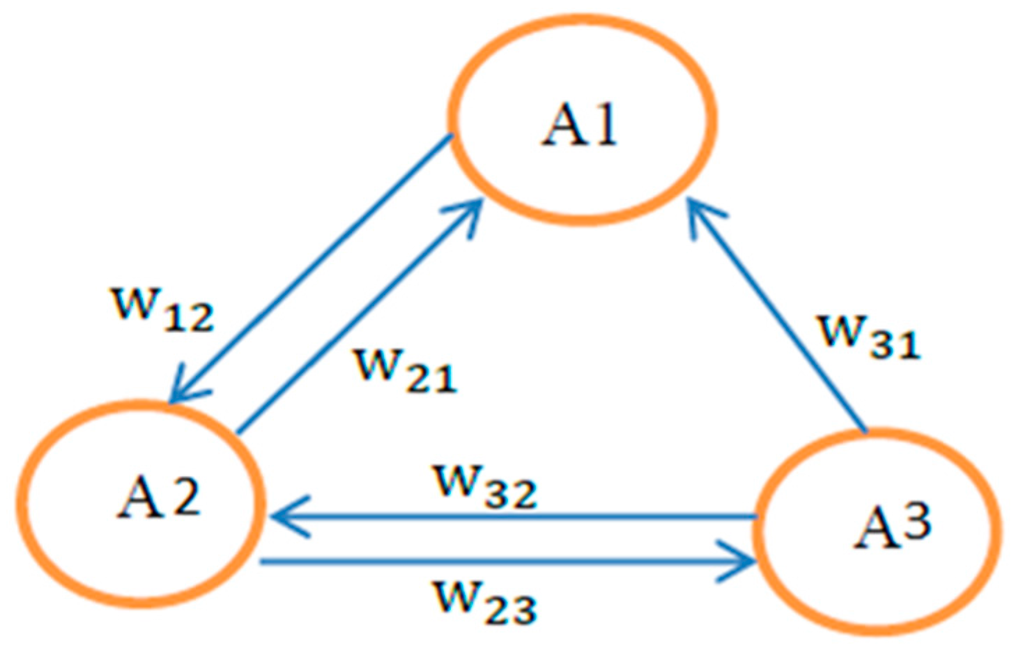
Figure 5 shows the graph structure of the proposed controller.
2.3.5. Allocating the Required Weights Based on the GPC Method
Assigning the proper weights for the FCM concepts could lead to better and fast convergence of the desired values. This way, the performance will be increased due to the fast convergence of FCM to the desired set points. The GPC method will be a suitable solution to allocate the weights for the actuators which are the control signals [
10]. As the FCM method is a type of fuzzy control method, all the weights should be normalized in the range of [−1, 1].
In the case of MIMO systems for finding the K matrix of GPC method, the steady space model is applied. Excluding the actuators, for other parameters of the system in FCM model, for converging the concepts to their operating point, the linearized model of the system is used around the operating point. In other words, the matrixes A and B of a steady space model are employed to describe the causal weights. If the concepts have direct relationships with each other, the values of the relations are adopted from matrixes A and B. For the other concepts with no relationship, if they have indirect relation with each other through the other concepts, the effect of the indirect relations should be used. At last, for the control signal concepts, the minimization values are calculated by GPC method to obtain the steady states (ss) or set points [
24]. By calculation of the minimum of the (
uk −
uss), the minimum control efforts are achieved. All the weights should be fuzzified in the range of [−1, 1]. In order to find the control law and closed loop poles of the system, the Equations (9)–(11) are used based on the steady space model of the system which is suitable for MIMO systems [
25]:
The K matrix is calculated based on the GPC model procedure which is calculated by minimization of the performance index.
2.3.6. Calculation of the Concepts Values
In the proposed controller, Equations (12) and (13) are used to derive the control law. The values of the fan’s flow rate and speed of compressor are calculated based on these two equations. The calculation procedure is continued until the calculated values in each iteration have no changes in comparison with the previous iteration. Then the calculation procedure stops.
Construction of FCM
In consideration of a required scenario for the control algorithm, the FCM is illustrated by a fuzzy-graph construction of a few nodes based on the requirement of the control system as concepts to represent causal reasoning [
26]. The system’s condition or characteristic is displayed by every single concept [
27].
Figure 6 indicates the diagram of FCM method as a graph structure.
The human knowledge about the operation of the system is represented by the FCM method and it can be developed based on the knowledge and experience of experts based on their experience about the model and behavior of the system [
28]. The type, number of concepts and relationships among the concepts are determined by experts. The system behavior is determined by main factors which are known by experts and shown by concepts in the FCM structure. Regarding the experts’ experiences, these concepts are extracted from the system’s events, values, actions, goals and tendencies [
29]. Based on the experts’ recognition and experiences, the relationships between the elements are defined and they can be improved by using suitable weights between the concepts. In other words, the experts’ knowledge about the system behavioral model is transformed in the form of weights. FCMs method is a combined method based on fuzzy logic method and artificial neural networks method which contains the robust characteristics of both methods [
27,
29].
The inputs and outputs of the system could easily be defined by the FCM method as nodes based on the control requirements of the system and expected operational scenario of the system. Thus, the MIMO approach could be met without the linearization of the system and limiting the operating range of the system. The other positive point of this structure is the causal relationship between the concepts in which the coupling effect between concepts could be considered as two side relationships between coupled parameters. This could improve the accuracy and sensitivity of the control system as close as the reality. Also, the definition of suitable range for the concept could prevent the overshoots and undershoots in the system. The FCM structure is able to define and limit the working range of the nodes, hence, the values of the nodes cannot exceed from these limits and may eliminate the overshoot and undershoot in the system. Moreover, the control law is derived from simple mathematics. The needs for measuring all states variables, additional measurements and a non-linear observer are omitted.
Mathematical Description of FCM
The structure of FCMs contains some concepts in which the value of each concept at a certain time is shown by A
i in the system which indicates the activation degree of the mentioned parameter. These values are achieved by transforming the real values of parameters into the interval [0, 1]. Weights among the concepts clarify the influence of parameters on each other and they are shown by
Wij. The values of weights are in the range from −1 to 1 [
27,
30].
The relations of the concepts are divided into three categories as positive which reveal same effect between the mentioned concept on the other one, Zero relation which represents no relationship between two concepts, and negative displays opposite effect of the mentioned concept on the other one [
27,
29,
30,
31]. This graphical structure of the FCM method follows the specific mathematical model as a 1 × n state vector (A) containing the values of the n concepts and an n × n weight matrix containing the weights (
Wij) of the relationship among the nodes. The number of concepts is shown by n [
32].
The value of every single concept depends on the linked concepts with suitable weights and besides the previous value of the mentioned concept. The values of the concepts should be transformed to their fuzzy values. The activation level of
Ai for every single concept are calculated as follows [
27,
29,
30,
31,
32,
33]:
Ainew clearly describes the concept
i activation value at time
t + 1.
Ajold specifies the concept
j activation value at time
t.
f is a sigmoid threshold function which compresses the values into the interval [0, 1] as follows [
27,
29,
30,
31,
32]:
2.3.7. Defuzzification of the Concept Values and Application to the Actuators
Finally, the values of the actuators should be anti-normalized and applied to the actuators. Defuzzification of the actuator values has been done by Equations (14) and (15):
2.4. Stability Analysis of the Fuzzy Cognitive Map Method
In order to analyze the stability of the FCM method, it should be consider as a one layer network Fuzzy Bidirectional Associative M emories (FBAMs) [
34]. In other words, it can be considered as a special case of FBAMs which has one layer network instead of a two layers network. The FBAM structure consists of a two-layer neural network. It has two layers X and Y. The connection matrixes from the X layer to the Y layer and vice versa are shown by matrix P and matrix R. The triangular norms are used to justify the stability analysis of FBAMs [
35]. The AND operation is generalized by triangular norms (T-norms) and the OR operation is generalized by T-conorm (S-norm). The connection matrixes between the layers are based on the max-T composition. If the S-T composition product of the connection matrixes converges to the max-T composition, the FBAM is globally stable. As the structure of FCM has one layer with one weight matrix, it can be considered as a two layers structure by decomposing the weight matrix (W) into the two triangular matrices [
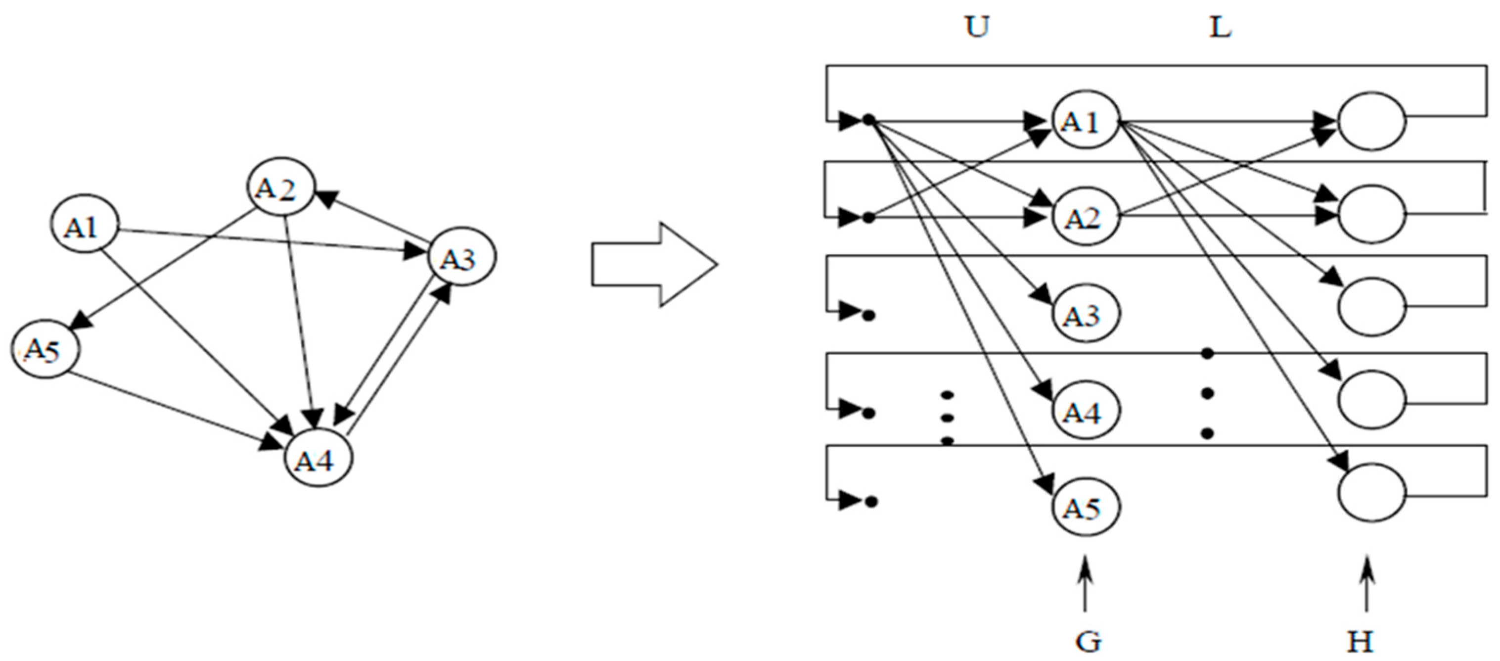
34].
The LU factorization method, or Gaussian elimination method are used to decompose the weight matrix of FCM. The matrix W is square, which it is the product of a permutation of a lower triangular matrix (L) with ones on its diagonal and an upper triangular matrix (U). The FCM weight matrix always can be decomposed into two triangular matrices due to the fuzzy values and directly and indirectly influence of the parameters on each other. The FCM structure is transformed into two-layers as layers G and H, which the connection between the layers are shown by L and U matrices. The L matrix shows the relationship from layer G to H, and the U matrix indicates it from layer H to G. Number of concepts for each layer is the same as FCM concepts.
Figure 7 shows the transformation of FCM structure into two layers designated as G and H [
34].
In order to prove the stability of FCM, a specific T-norm should exist from the S-T composition of the
L and
U matrices which should be equal to the original weight matrix. If this S-T composition exists, the FCM is globally stable. The product of S-T composition for two matrices
L = (
lij)
m ×
p and
U = (
uij)
p ×
n should be as follows [
34]:
Therefore, for the proposed designed controller, the weight matrix and factorization to the matrix L and U is as below. Consequently, as the weight matrix is the product of S-T composition of L and U matrices based on Equation (17), the designed controller is globally stable.
3. Results
In this paper, the results of the controller are attained for the conditions of tropical countries like Malaysia, where the average air temperature is 30 °C and the humidity is 80%. This controller is able to reduce the temperature to 25 °C (this is in the acceptable range of thermal comfort temperature for tropical countries according to American Society of Heating, Refrigerating, and Air-Conditioning Engineers (ASHRAE) [
36]) and the humidity to 50% (also in the acceptable range of comfort humidity for tropical countries defined by ASHRAE [
36]) [
37,
38,
39]. The results in this section consist of three parts: set point tracking, performance analysis test by reference tracking by changing the set point and disturbance rejection, and finally, the comparison of the energy usage of the system in neighborhood of operating point for both the proposed GPC-FCM controller and the LQG controller from [
8].
3.1. Set point tracking
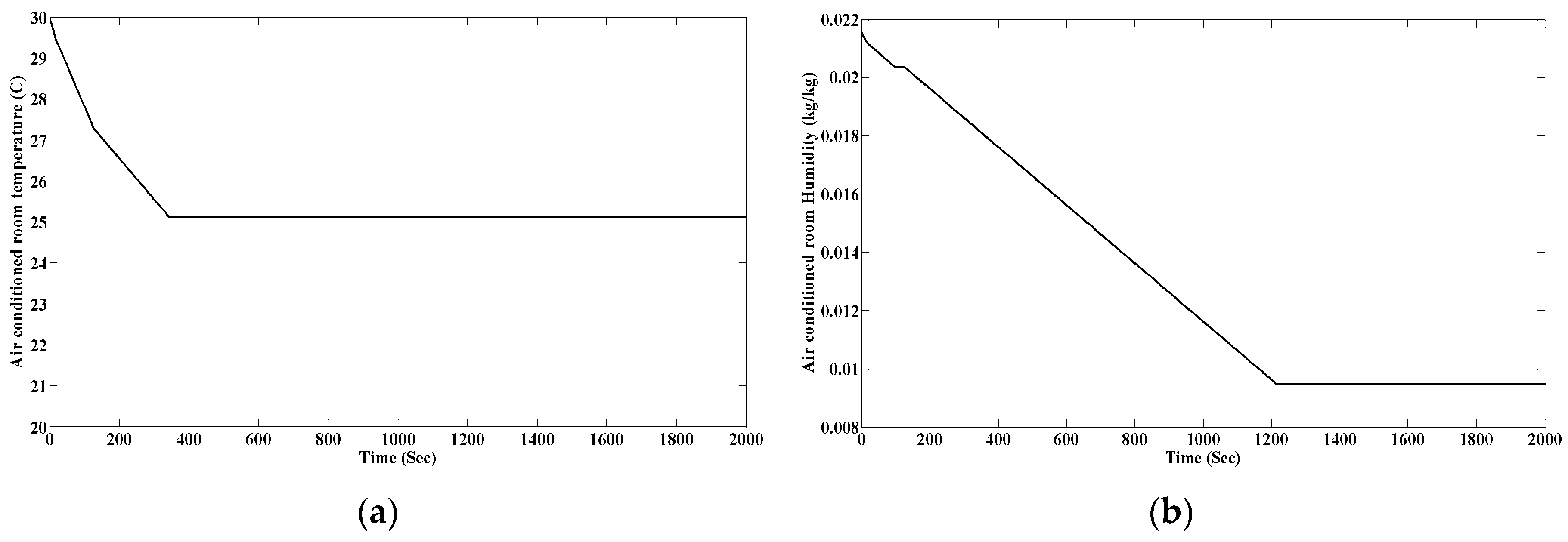
The air-conditioned room temperature is indicated in
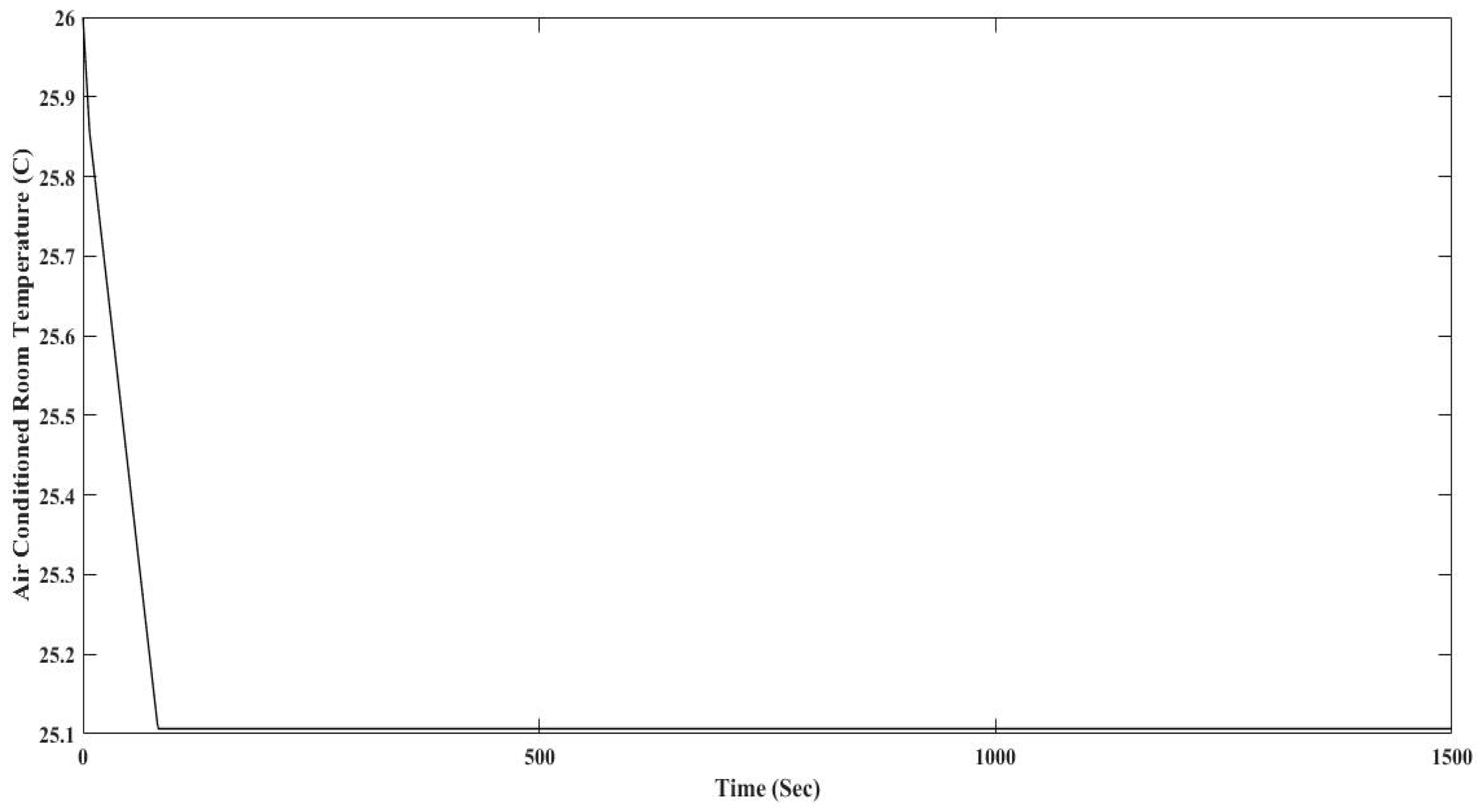
Figure 8a. By changing the compressor speed and supply fan flow rate, the temperature of the air-conditioned room decreased from 30 °C to 25.1 °C at 380 s. The air-conditioned room temperature reached to the desired set point in 6.3 min with 0.33% error and the temperature maintained at the desired set point.
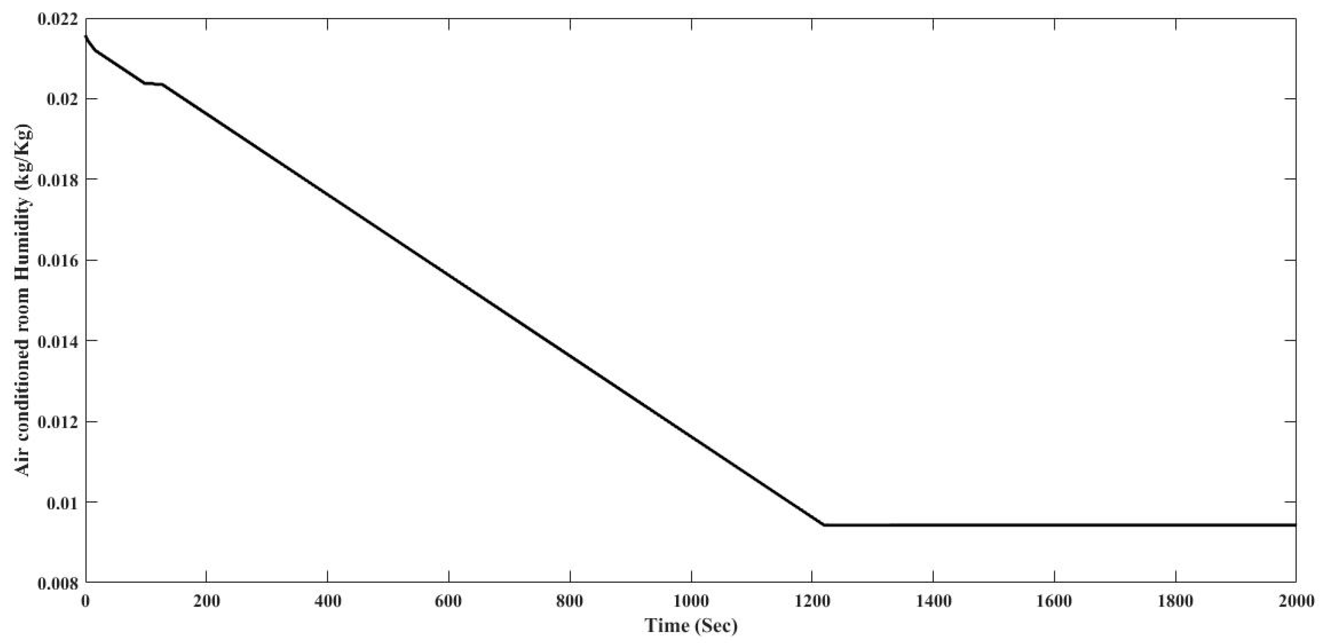
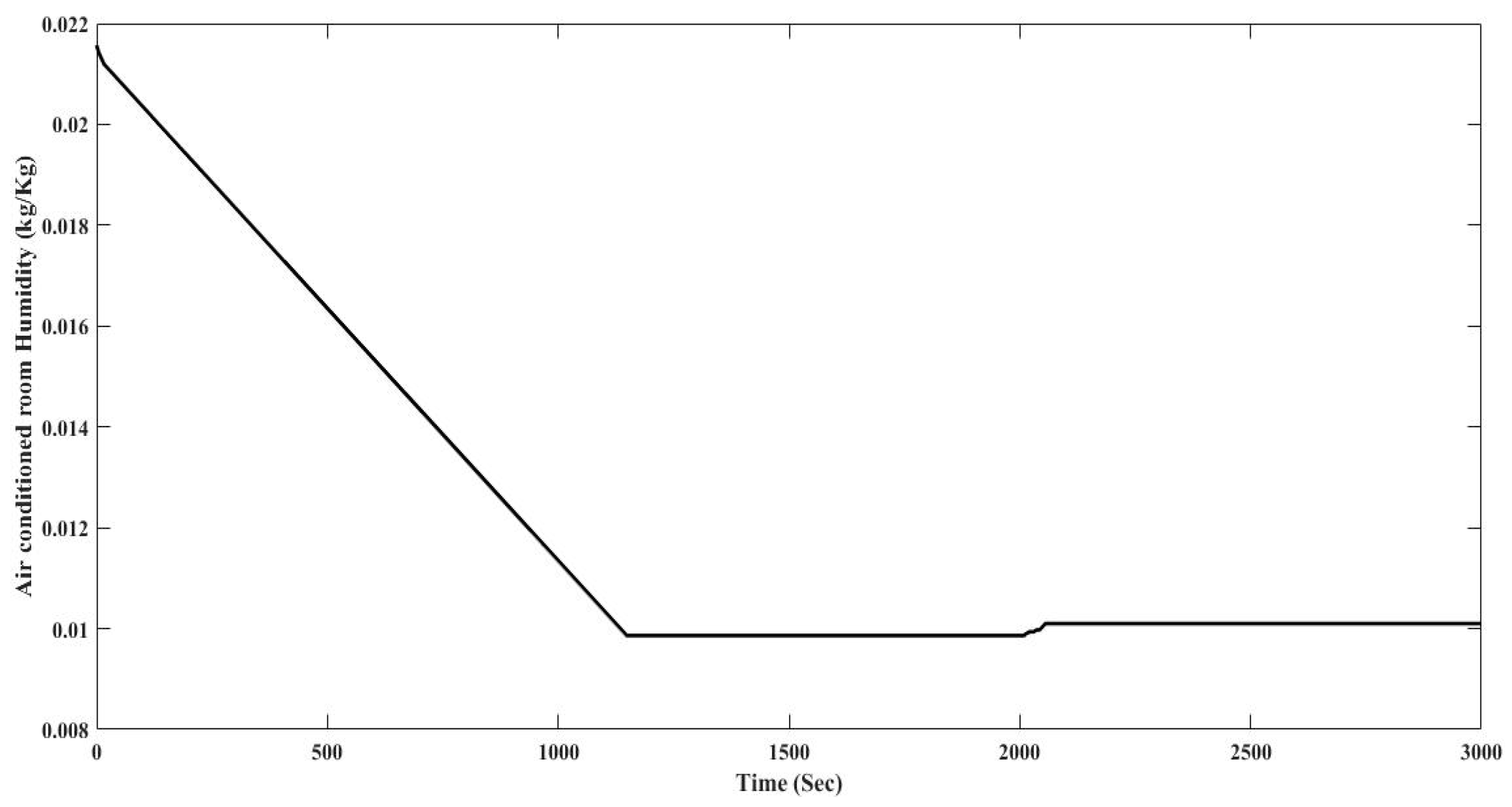
Figure 8b shows the air-conditioned room humidity which is decreased from 0.02157 kg/Kg to 0.00948 kg/Kg at 1200 s. By changing the speed of compressor and supply fan’s flow rate, the air-conditioned room humidity decreased from 80% humidity to 48% humidity in 20 min with a 2.5% error from 50% humidity. The comfort humidity range of air-conditioned room in tropical countries is between 40% and 60%. Then, the air-conditioned room humidity stabilized at 0.00948 kg/Kg.
Figure 9a indicates the flow rate of the fan. In order to decrease the air-conditioned room temperature and humidity, the fan’s flow rate increased from 0.34 m
3/s to 0.382 m
3/s and more or less stabilized around 0.382 m
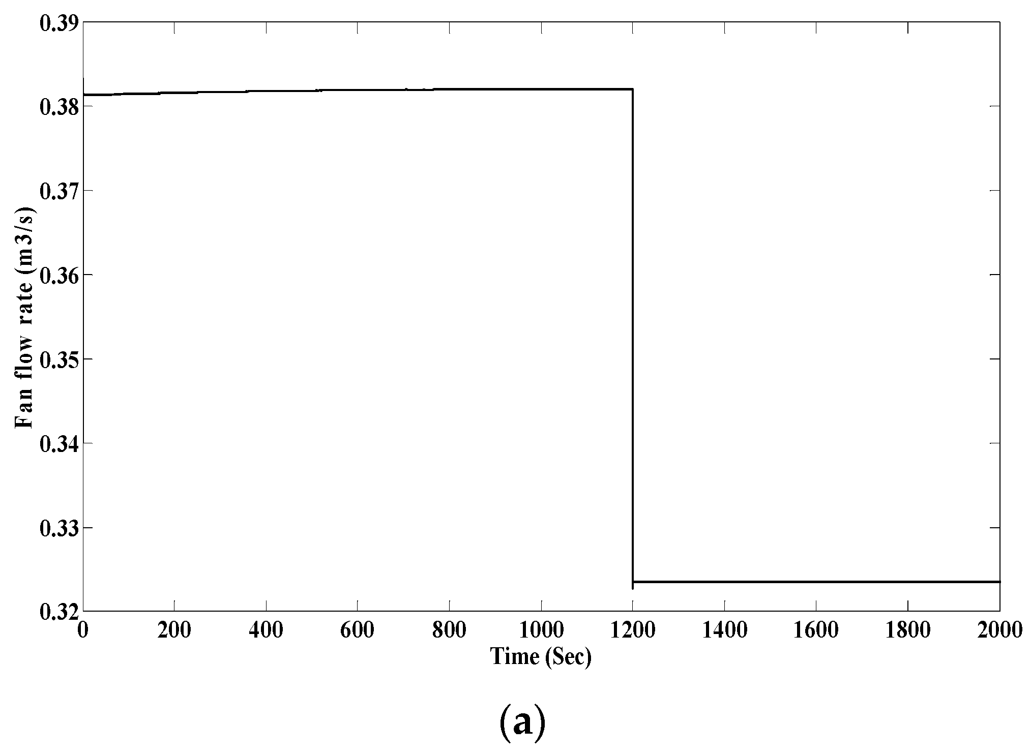
3/s and kept this flow rate until the temperature and humidity of the room reached the desired set points at 1173 s. When the temperature and humidity of the room reached to the desired values at 1173 s, the flow rate of the fan declined and maintained at 1200 s at 0.325 m
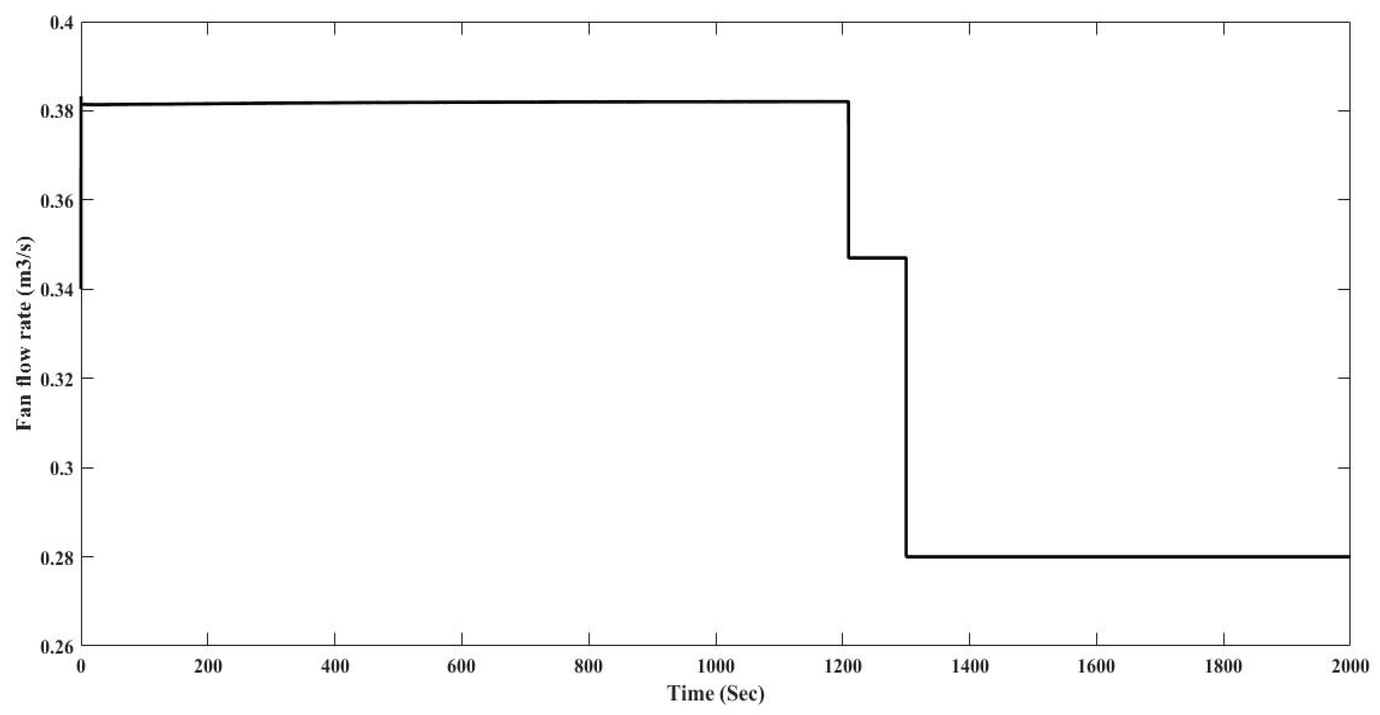
3/s which is the minimum required value for the flow rate of the fan to keep the condition of the air-conditioned room in desired set points.
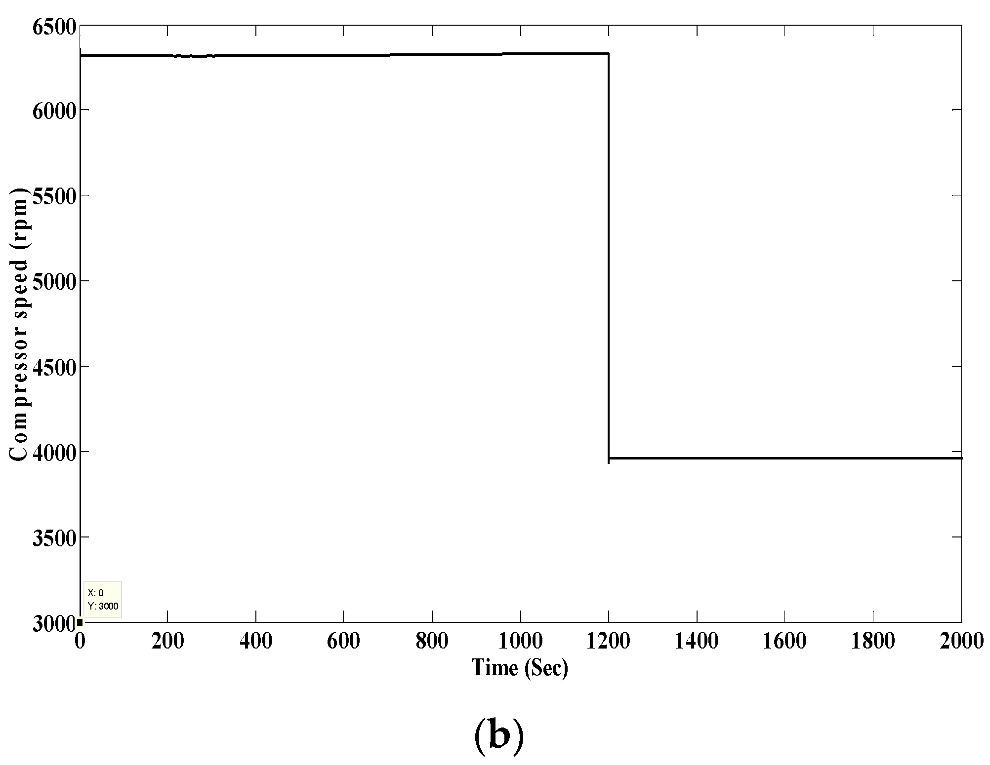
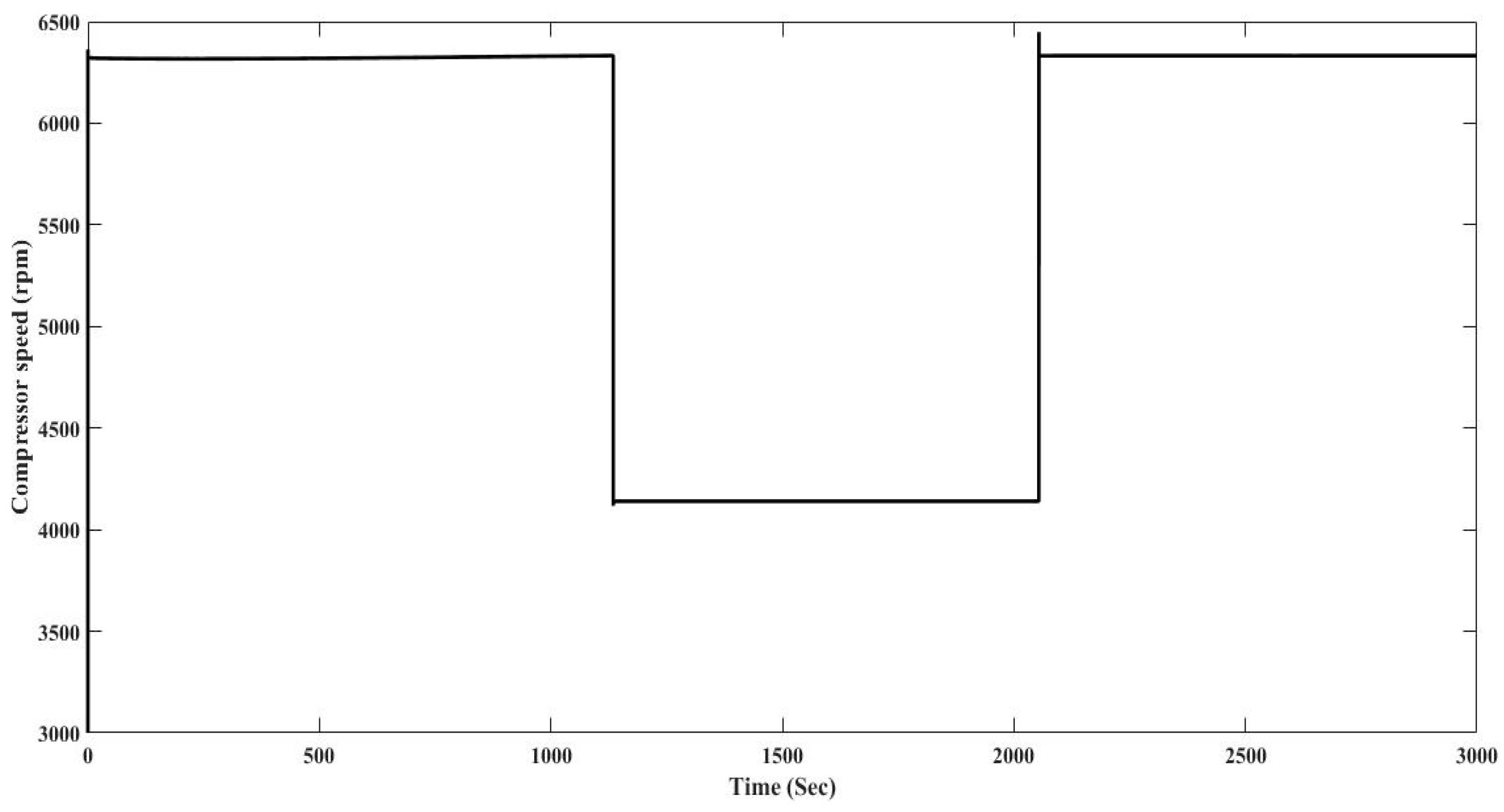
Figure 9b illustrates the compressor speed which increased from 3000 rpm to 6359 rpm and approximately stabilized about 6320 rpm for declining the air-conditioned room temperature and humidity of. Then, from 1173 s to 1200 s, the speed of the compressor decreased and maintained at 3960 rpm to keep the air-conditioned room temperature and humidity in desired set points.
3.2. Performance Analysis
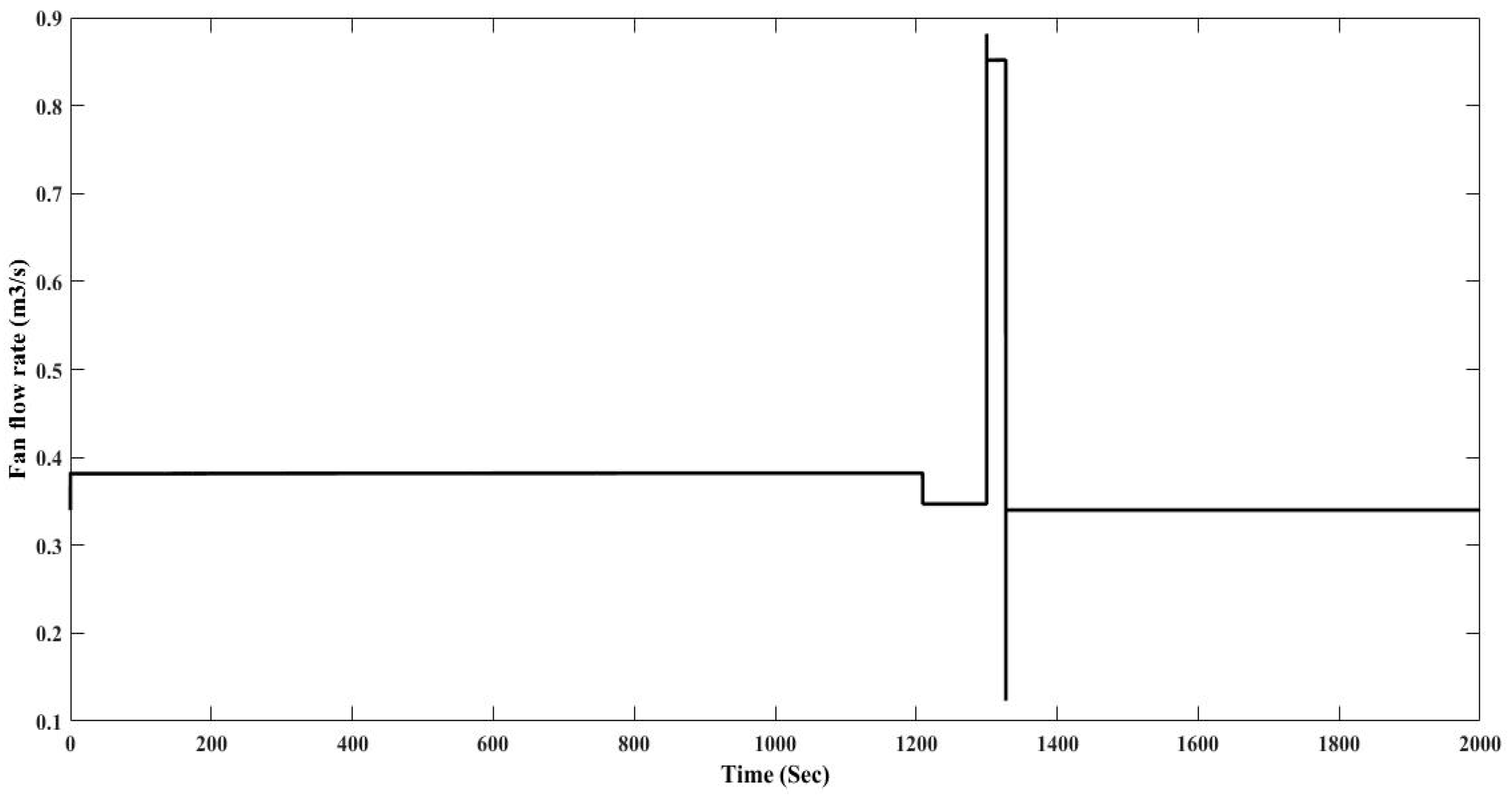
The performance and ability of the proposed controller was tested by two tests. The first test is set point tracking in which the set point was changed from 25 °C to 23 °C, and also from 25 °C to 26 °C at 1300 s. The second test is disturbance rejection test in which the values of the disturbances which are heat load and moisture load (Qload and M) were changed from 4.49 kW and 0.96 Kg/s to 5.49 kW and 1.6 Kg/s respectively at 2000 s.
3.2.1. Reference Tracking by Changing the Set Point
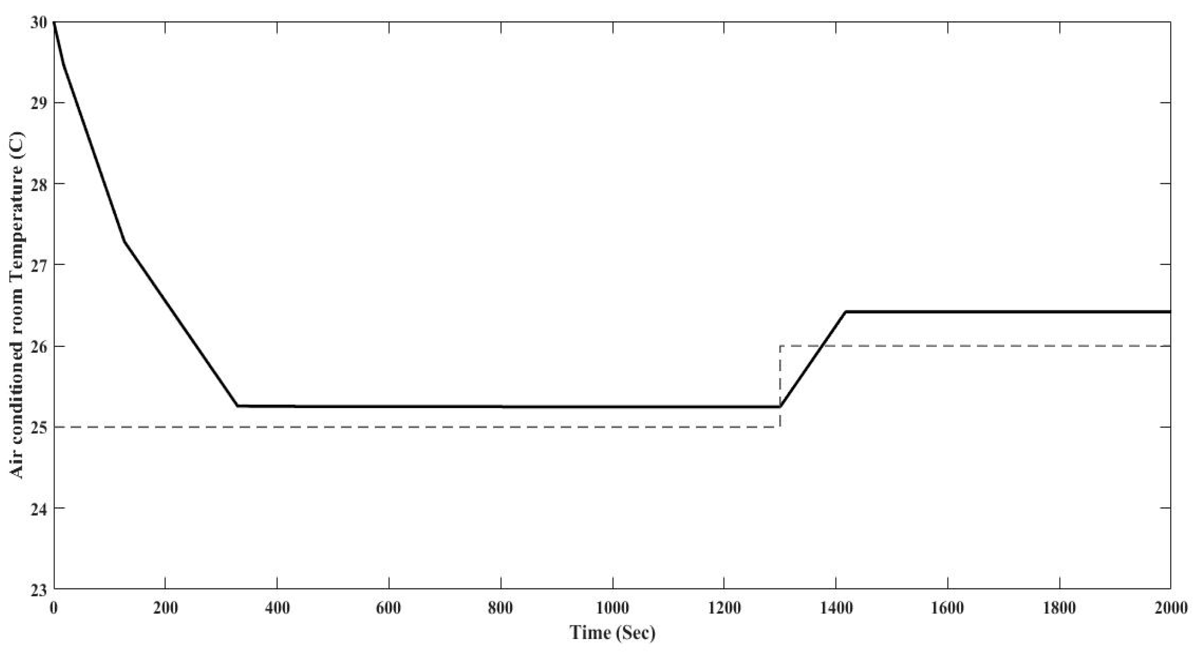
In order to show the ability of the controller, in the following set point tracking test the set point increased from 25 °C to 26 °C which is explained in the text in S3.
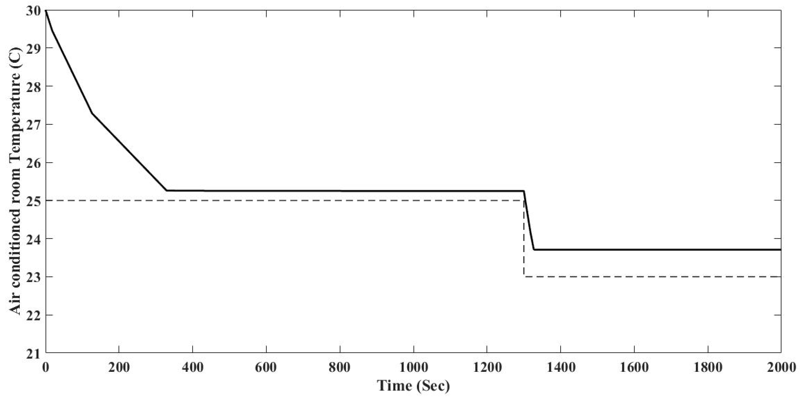
Figure 10 shows the reference and actual temperature of the air-conditioned room. There is a change in the reference temperature from 25 °C to 26 °C at 1300 s. The initial room temperature is at 30 °C. It can be clearly seen that the proposed controller stabilized the temperature of the air-conditioned room at the first desired set point at 329 and stabilized the temperature at the second desired set point at 1417 s, which is exactly 117 s after changing the set point. By decreasing the fan’s flow rate and speed of the compressor, in 117 s the air conditioned room temperature increased and reached to the new set point. By changing the speed of compressor and supplying fan flow rate, the temperature of the air-conditioned room increased from 30 °C to 25.1 °C for the first set point at 380 s. The temperature reached to the desired set point in 6.3 min with 0.33% error and the temperature kept at the desired set point until 1300 s that the set point changed to the new one. For the second set point, the temperature of the air-conditioned room decreased from the 25.1 °C to 26.42 °C in about 117 s and stabilized with 1.4% error from set point.
The humidity of the air-conditioned room is demonstrated in
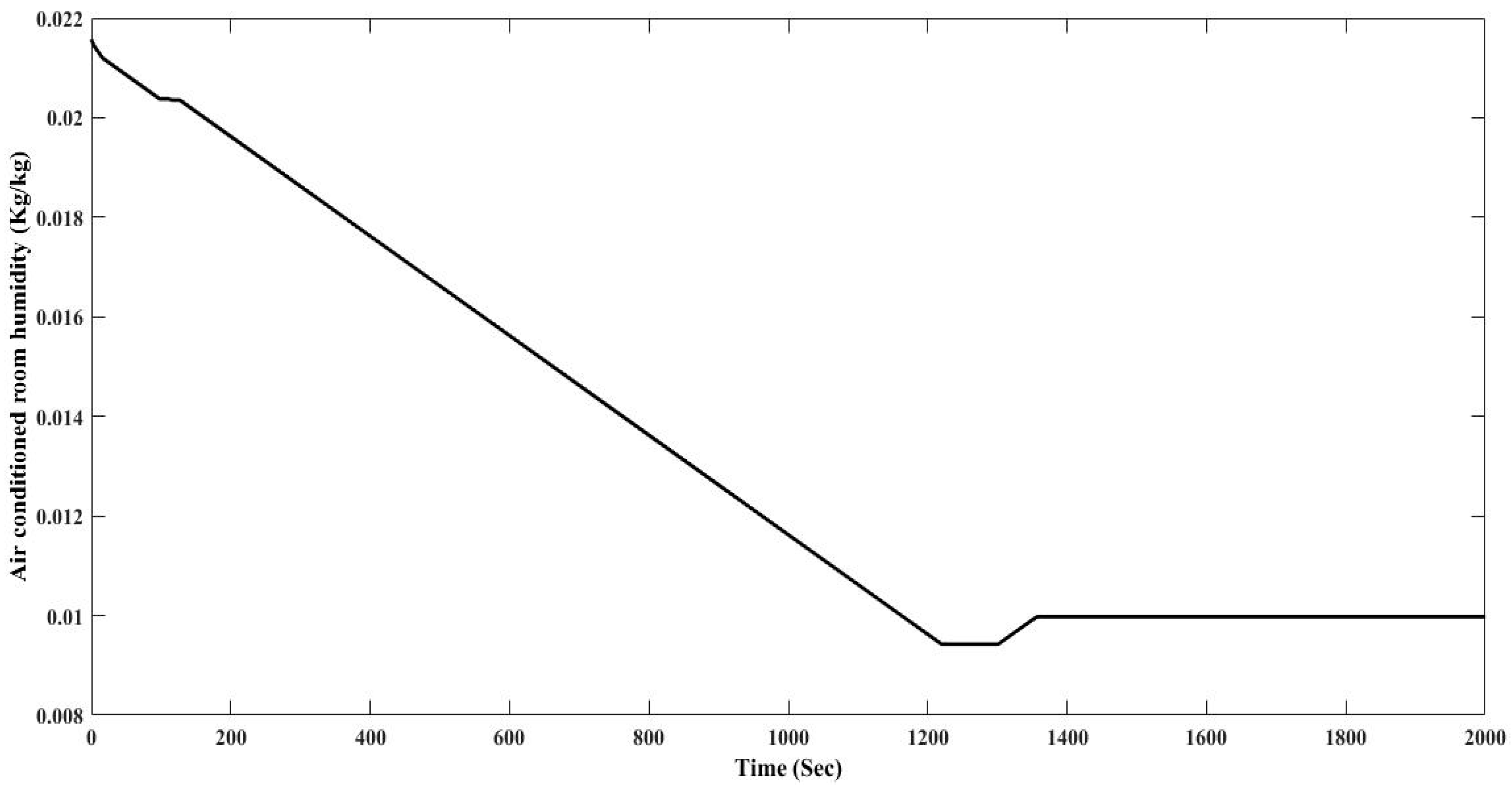
Figure 11. The initial room humidity is set at 0.02157 kg/Kg or 80%. It can be clearly seen that the proposed controller stabilized the humidity at the desired set points in about 1221 s. By changing the compressor speed and supply fan flow rate, the humidity of the air-conditioned room declined from 80% or 0.02157 kg/Kg to 45% or 0.009425 kg/Kg at about 1221 s or 20. 35 min and stabilized with 6.25% error from 50% humidity. The humidity is still in the acceptable comfort range for the humidity in tropical regions that is in the domain of 40% to 60%.
The flow rate of the fan is indicated in
Figure 12. The initial flow rate is at 0.34 m
3/s. It is clear that the proposed controller stabilized the flow rate at 700 for the first set point and after changing the set point at 1300 s, it is stabilized at 1320 s which is exactly 20 s after changing the set point. For the first set point, by increasing the fan’s flow rate from 0.34 m
3/s to 0.382 m
3/s, the temperature and humidity of the air conditioned room decreased to 25.1 °C and 48% humidity and stabilized the flow rate of the fan at about 700 s and kept until 1173 s. After reaching to the desired set point, the flow rate of the fan decreased to 0.3468 m
3/s from 1173 s to 1200 s and kept stable until 1300 s. Due to the set point changing at 1300 s, in order to reach to the new set point, the flow rate of the fan decreased to 0.28 m
3/s, then when the temperature of the room reached to the new set point, the flow rate of the fan decreased to the minimum required value to keep the temperature and humidity of the room at desired set points, and finally stabilized at 0.28 m
3/s at around 1320 s and maintained.
The speed of the compressor is illustrated in
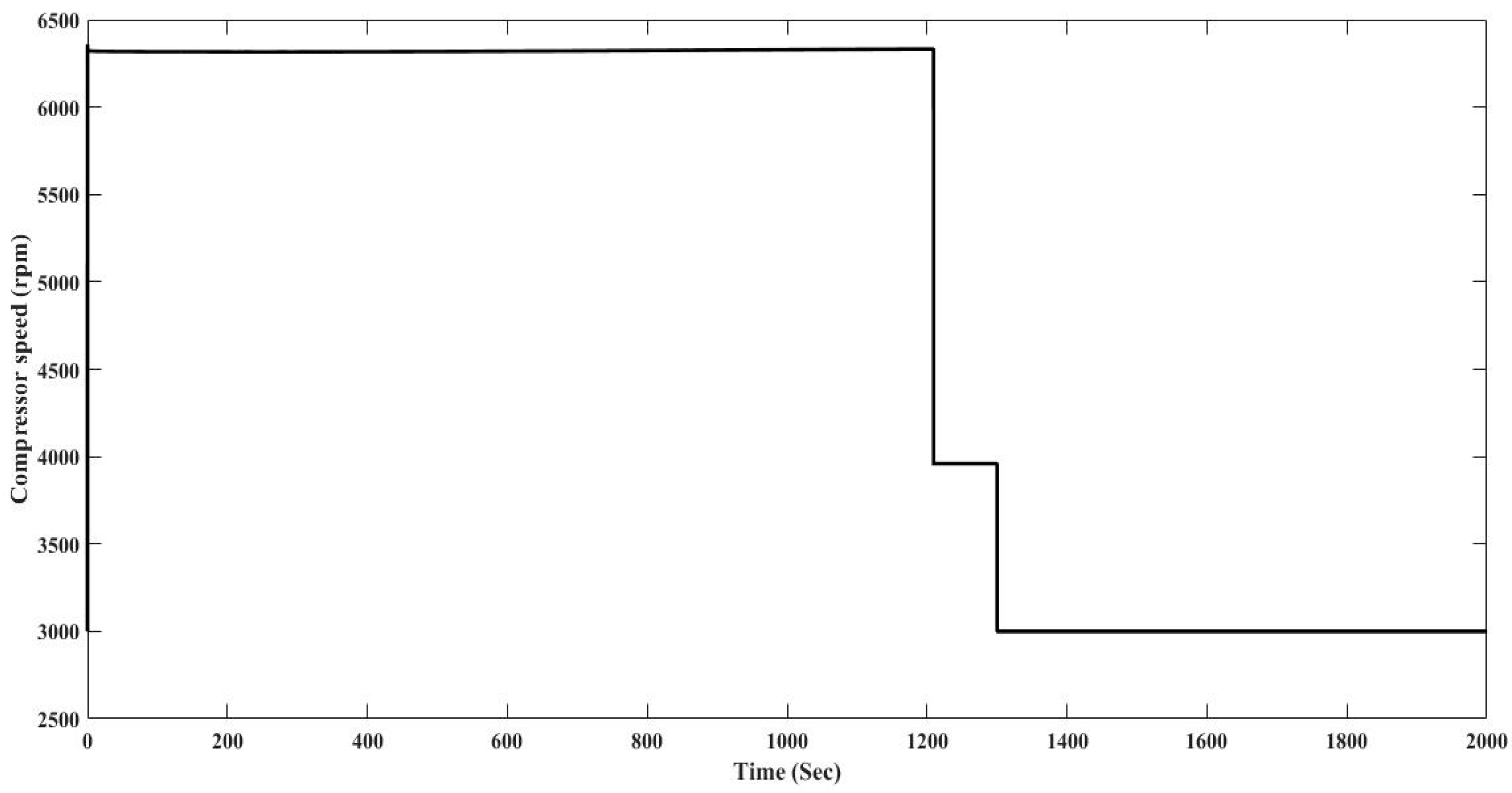
Figure 13. The initial speed of the compressor is at 3000 rpm. It is clear that the proposed controller stabilized for first set point of the compressor speed at 1209 and for the second set point at 1320 s, which is exactly 20 s after changing the set point. By increasing the compressor speed from 3000 rpm to 6359 rpm and keeping the situation around 6330 rpm stable, the temperature of the room reached to the first set point at around 1200 s. After reaching to the desired set point, the compressor speed decreased and maintained at 3949 rpm which is the minimum required value to keep the condition from 1200 s to 1300 s. After set point changing at 1300 s, the compressor speed decreased to 3000 rpm in order to reach to the new set point. When the temperature of the room reached to the new set point, the compressor speed decreased from 1300 s to 1320 s and maintained on 3000 rpm to keep the condition of the room.
Figure 14 shows the reference and actual temperature of the air-conditioned room. There is a change in the reference temperature from 25 °C to 23 °C at 1300 s. The initial room temperature is at 30 °C. It can be clearly seen that the proposed controller stabilized the temperature of the air conditioned room at the first desired set point at 380 s and stabilized the temperature at the second desired set point at 1325 s, which is exactly 25 s after changing the set point. By increasing the flow rate of the fan and compressor speed, in 25 s the temperature of the air-conditioned room decreased and reached to the new set point. By changing the compressor speed and supply fan flow rate, the temperature of the air-conditioned room decreased from 30 °C to 25.1 °C for the first set point at 380 s. The temperature reached to the desired set point in 6.3 min with 0.33% error and the temperature maintained at the desired set point until 1300 s that the set point changed to the new one. For the second set point, the air-conditioned room temperature decreases from 25.1 °C to 23.6 °C in about 25 s and stabilized with 2% error from the set point.
The humidity of the air-conditioned room is illustrated in
Figure 15. The initial room humidity is at 0.02157 kg/Kg or 80%. It can be clearly seen that the proposed controller stabilized the humidity at the first desired set point at 1200 s and stabilized the humidity at the second desired set point at 1357 s, which is exactly 57 s after changing the set point. The humidity declined from 80% or 0.02157 kg/Kg to 48% or 0.00948 kg/Kg at about 1200 s. After changing the set point at 1300 s the humidity reached to 0.009977 kg/Kg or 53.5% at 1357 s and stabilized. By changing the compressor speed and supply fan flow rate, the air-conditioned room humidity decreased from 80% humidity to 48% humidity in 20 min with 2.5% error from 50% humidity for the first set point and for the s set point it reached to the desired set point in about 1 min with 4.3% error from 50% humidity. The humidity is still in the acceptable comfort range for humidity in tropical regions that is in the domain of 40% to 60%.
The flow rate of the fan is indicated in
Figure 16. The initial flow rate is at 0.34 m
3/s. It is clear that the proposed controller stabilized the flow rate at 1200 for the first set point and after changing the set point at 1300 s, it is stabilized at 1339 s, which is exactly 39 s after changing the set point. For the first set point, by increasing the fan’s flow rate from 0.34 m
3/s to 0.382 m
3/s, the temperature and humidity of the air-conditioned room decreased to 25.1 °C and 48% humidity and stabilized the flow rate of the fan until 1173 s. After reaching to the desired set point, the flow rate of the fan decreased to the to 0.325 m
3/s from 1173 s to 1200 s and kept stable until 1300 s. Due to the set point changing at 1300 s, in order to reach to the new set point, the flow rate of the fan increased to 0.8815 m
3/s, then when the temperature of the room reached to the new set point, the flow rate of the fan decreased to the minimum required value to keep the temperature and humidity of the room at desired set points and finally stabilized at 0.34 m
3/s at around 1339 s and remained maintained.
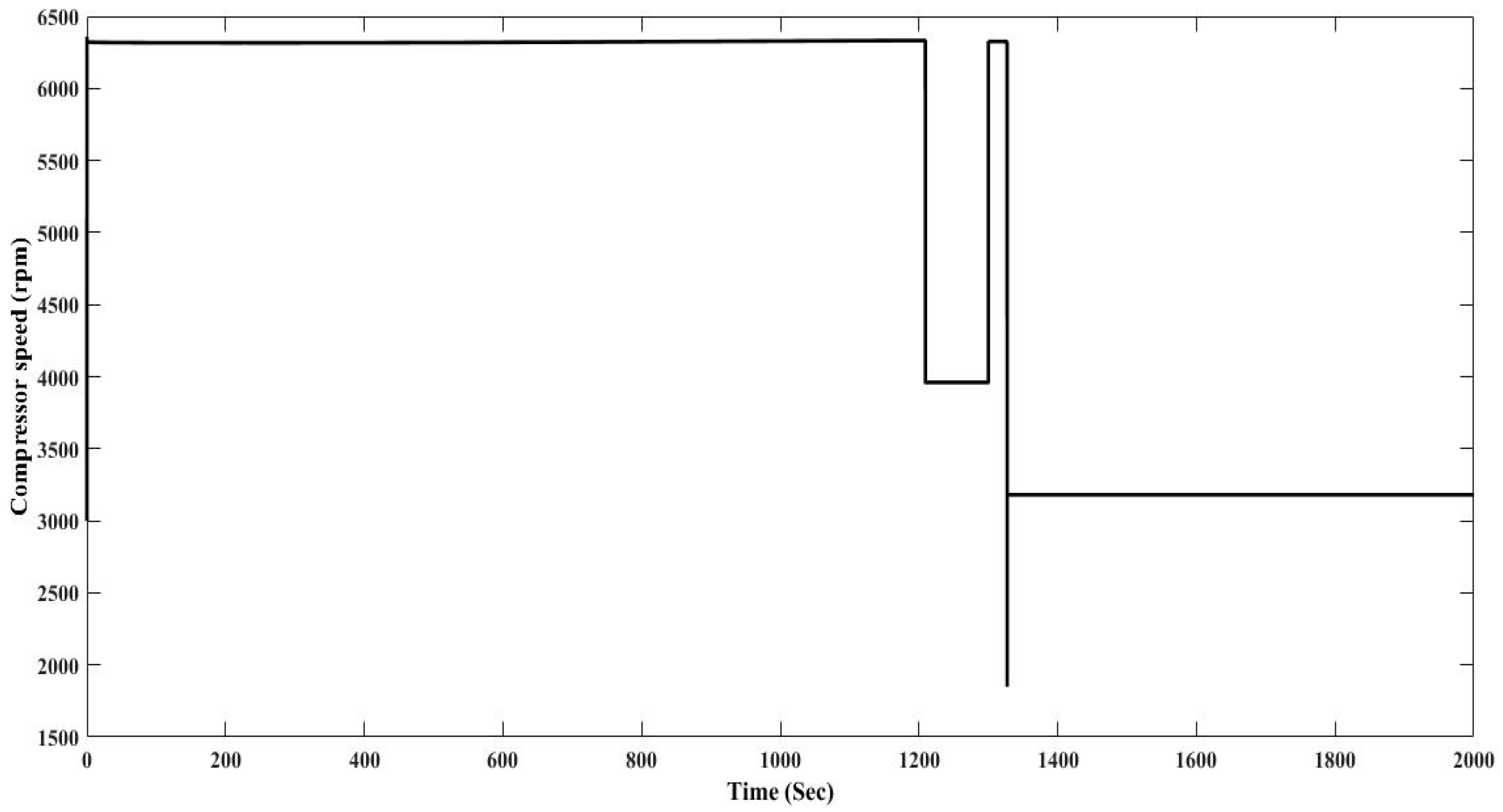
The speed of compressor is illustrated in
Figure 17. The initial speed of the compressor is set at 3000 rpm. It is clear that the proposed controller stabilized the first set point of the compressor speed at 1200 and for the second set point at 1334 s, which is exactly 34 s after changing the set point. By increasing the compressor speed from 3000 rpm to 6359 rpm and kept stable the situation around 6320 rpm, the temperature of the roomed reach to first set point at around 1200 s. After reaching to the desired set point, the compressor speed decreased and maintained at 3960 rpm which is the minimum required value to keep the condition from 1200 s to 1300 s. After the set point changing at 1300 s, the compressor speed raised to 6326 rpm in order to reach to the new set point. When the temperature of the room reached to the new set point, the compressor speed decreased from 1327 s to 1334 s and maintained on 3180 rpm to keep the condition of the room.
3.2.2. Disturbance Rejection
The results in this section emphasize on the ability of the controller to control and maintain the outputs of the system at desired set points in the presence of disturbances. In this case, by varying the supply fan flow rate and speed of the compressor, the air-conditioned room temperature and humidity have been controlled and maintained at the desired set points. In this test, at 2000 s the heat load and moisture load changed from 4.49 kW and 0.96 Kg/s to 5.49 kW and 1.6 Kg/s, respectively.
The air-conditioned room temperature with disturbance rejection is shown in
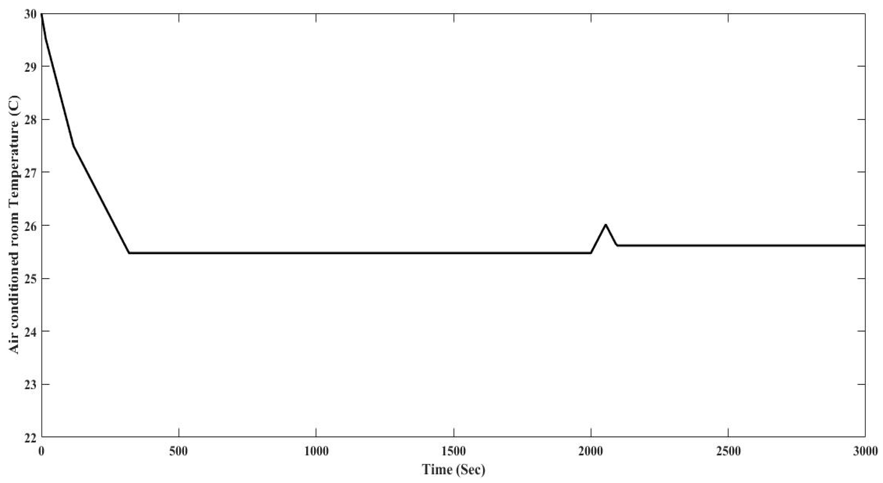
Figure 18. At 2000 s by increasing the heat load in the room, the air-conditioned room temperature increased gradually and at around 2050 s. Due to the increasing air-conditioned room, the temperature and exceed from the acceptable range for desired set point, the speed of the compressor and supply fan increased to reject the disturbances in the room. By increasing the compressor speed and flow rate of the fan, the temperature of the room started to decrease slowly and at 2100 s maintained at 25.6 °C which is in the acceptable range. The disturbances rejected and the temperature reached to the desired set point in 1.66 min with 2% error and the temperature maintained at the desired set point.
By increasing the moisture load at 2000 s, the air-conditioned room humidity increased slowly from 0.009863 kg/Kg to 0.01008 kg/Kg at around 2050 s and reached to the 0.0101 kg/Kg and maintained which is indicated in
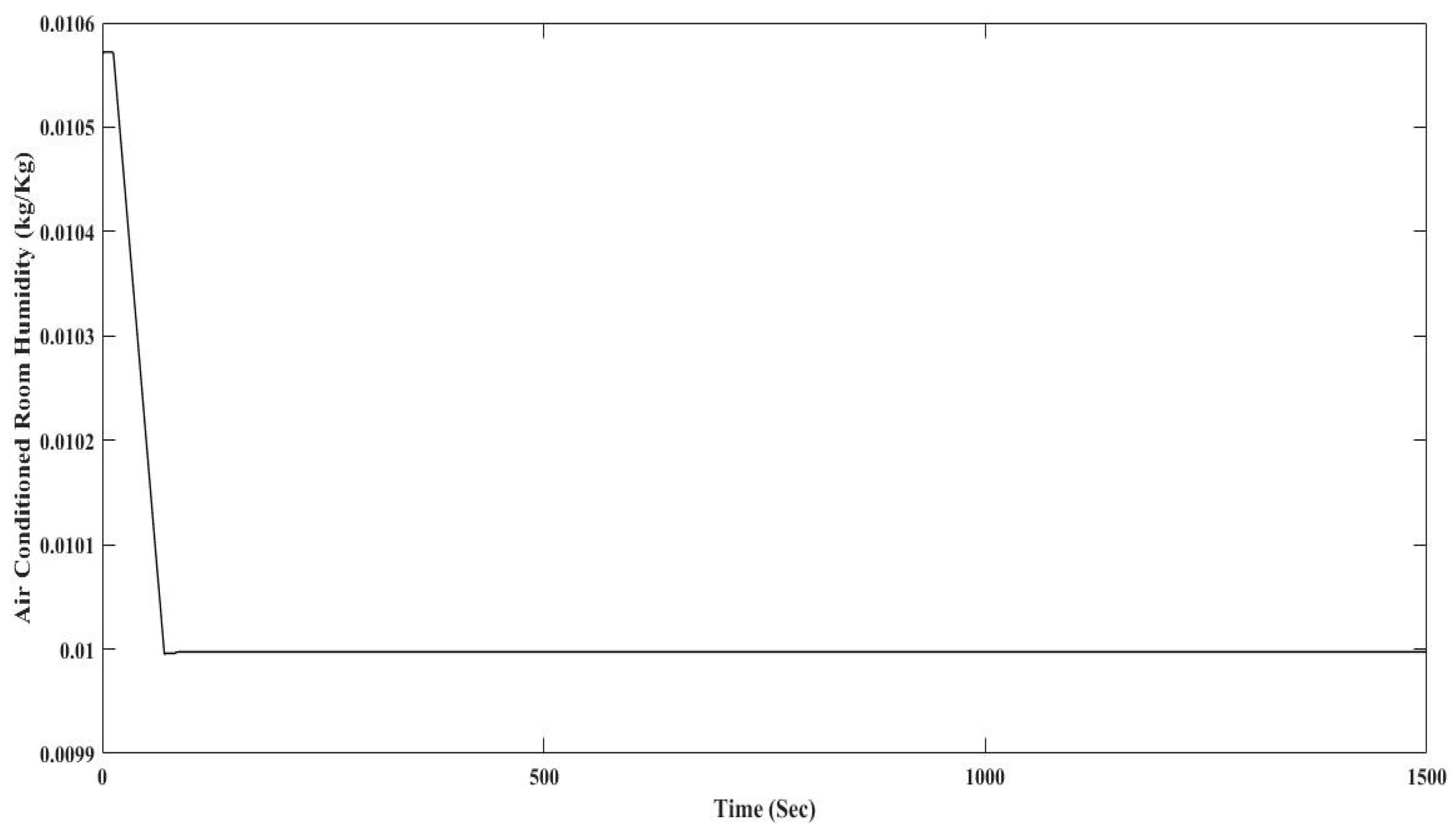
Figure 19. By increasing the speed of compressor and flow rate of the fan, the disturbances rejected and the humidity of the room kept at 49.5% humidity which is at the acceptable range for the air-conditioned room humidity. The humidity kept at desired set point with 0.625% error from 50% humidity.
In
Figure 20 the flow rate of the supply fan is indicated. By increasing the moisture and heat load in room at 2000 s, the temperature and humidity of the room increased, then as they exceed their acceptable ranges for the desired set points, the flow rate of the fan increased sharply from 0.341 m
3/s at 2046 s to 0.4595 m
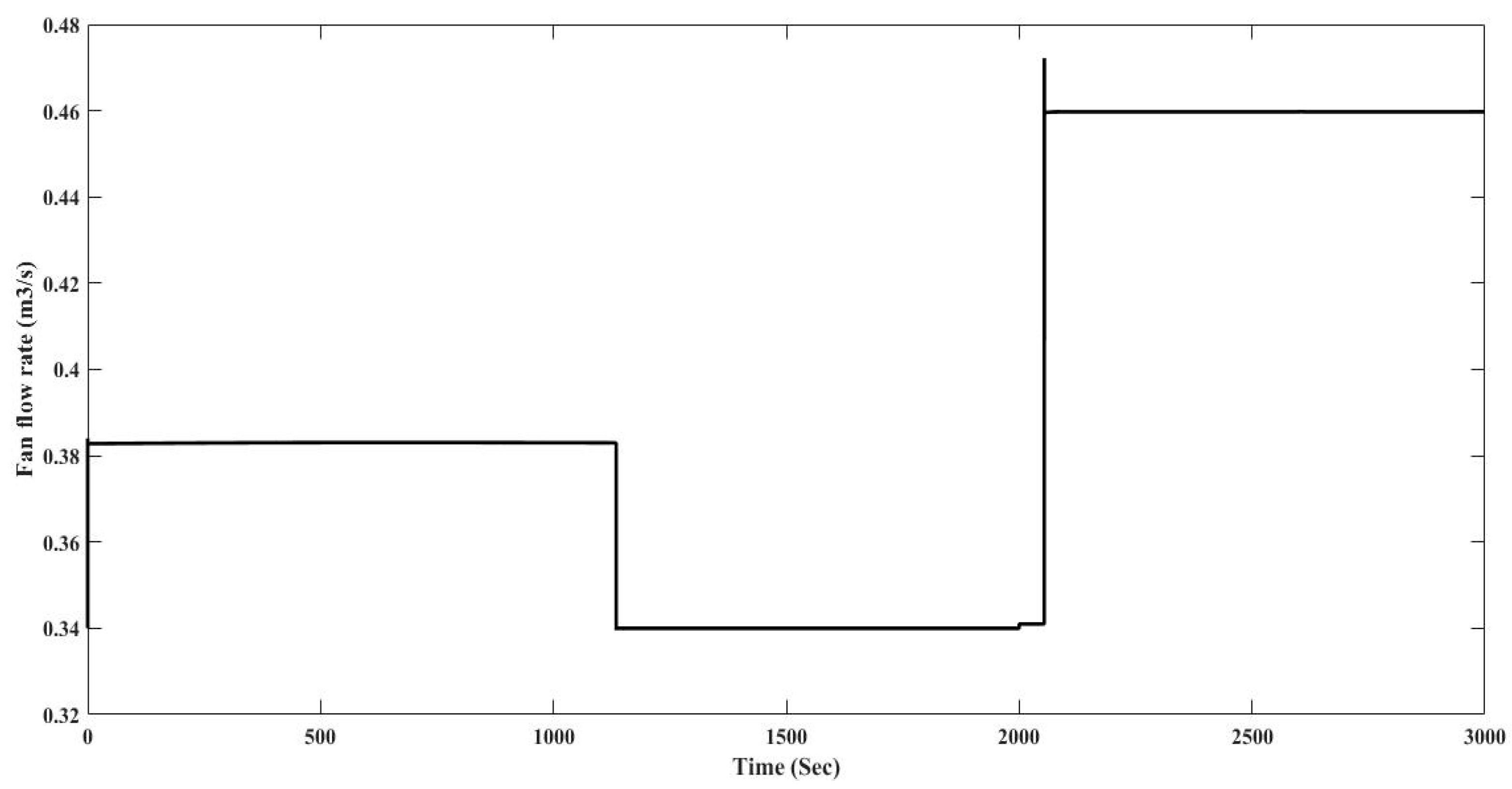
3/s at 2066 s and remained at this value which is the minimum required value to reject the disturbances and keep the temperature and humidity of the room at desired set points.
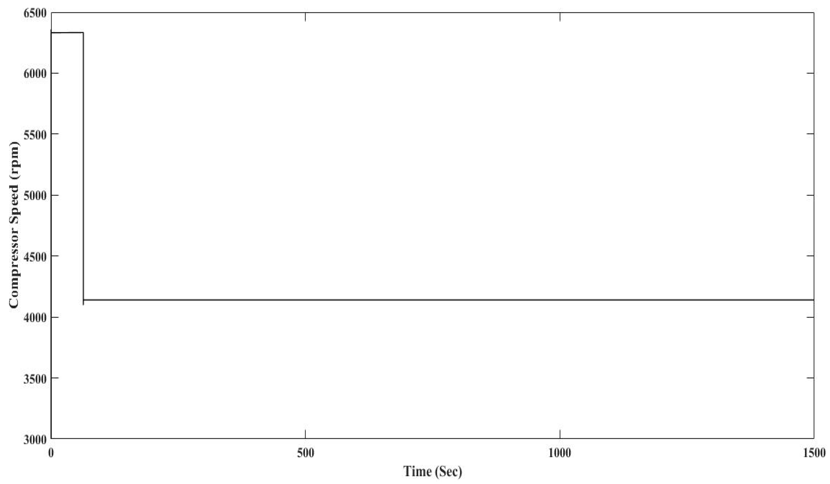
Figure 21 shows the compressor speed. By increasing the moisture and heat load in room at 2000 s, the temperature and humidity of the room increased, then as they exceed from their acceptable ranges for desired set points, the compressor speed increased from 4140 rpm at 2054 s to 6332 rpm at about 2066 s and became stable at this value which is the minimum required value to reject the disturbances and keep the temperature and humidity of the room at desired set points.
3.3. Comparison the Energy Consumption and Performance Indexes of GPC-FCM with LQG
This section compares the obtained results based on the proposed GPC-FCM controller with LQG controller based on [
8] works. The comparison of results by GPC-FCM controller with the LQG controller is not arbitrary. As a suitable criterion to compare the GPC-FCM controller results on the same system, the LQG controller which is the previous work on this system is chosen. In order to compare the performance of both controllers, performances and energy consumption of them which are applied on the same DX A/C system are compared in the same condition. As the LQG controller was designed as a MIMO controller on the linearized model of the system, it can only work properly around the operating point of the system. In order to compare both controllers, they were tested under the same conditions around the operating point. The initial air conditioned room temperature is considered 26 °C and the initial air conditioned room humidity is considered 0.01057 kg/Kg and the desired temperature and humidity are considered 25 °C and 0.00988 kg/Kg, respectively. In the same situation, the energy consumption of both controllers was calculated.
The temperature of the air-conditioned room by GPC-FCM controller is shown in
Figure 22. The temperature decreased from 26 °C to 25.1 °C in about 82 s and remained steady. By increasing the compressor speed and flow rate of the fan by increasing the supply fan speed, the temperature decreased from 26 °C to 25.1 °C in about 82 s. The temperature reached the desired set point in 1.36 min with 0.33% error and the temperature was maintained at the desired set point.
Figure 23 indicates the air conditioned room humidity by GPC-FCM controller which is decreased from 0.01057 kg/Kg to 0.00999 kg/Kg in about 70 s and maintained. By increasing the speed of compressor and fan’s flow rate by increasing the supply fan speed, the air conditioned room humidity decreased from 50% humidity for 26 °C to 50% for 25.1 °C in 1.16 min with no error from 50% humidity.
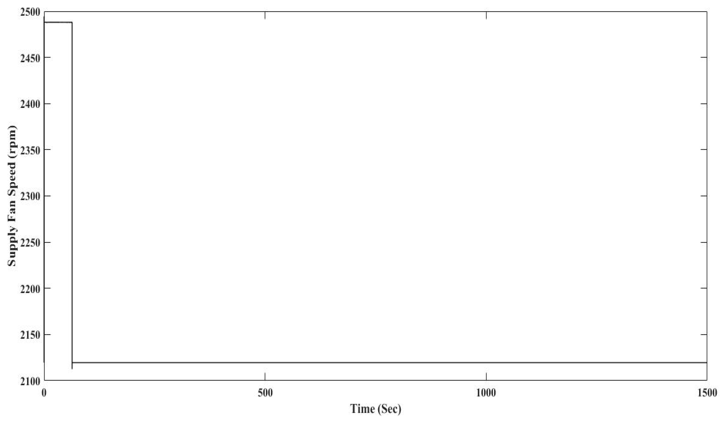
The speed of the supply fan is indicated in
Figure 24. The speed of the fan increased from 2120 rpm to 2488 rpm and was maintained at 63 s, then it decreased to 2120 rpm at 72 s and was maintained. At 63 s when the temperature of the room reached to the desired values, the speed of the fan started to decrease until it reached to the required speed for keeping the air-conditioned room temperature and humidity at the desired set points. The speed of the fan decreased to 2120 rpm at 72 s and maintained the speed.
Figure 25 shows the speed of the compressor. To decrease the temperature of the air-conditioned room, the compressor speed increased from 3000 rpm to 6333 rpm in 10 s and was then maintained until 62 s, then by declining the air-conditioned room temperature to the desired value, the speed of the compressor decreased and maintained at 4140 rpm at 74 s and maintained to keep the air conditioned room temperature and humidity in desired set points.
In 1500 s, the energy usage by compressor is 6.349 × 10⁶ (W) and energy usage by supply fan is 3.203 × 10⁶ (W). The total energy usage by applying GPC-FCM controller is 9.552 × 10⁶ (W).
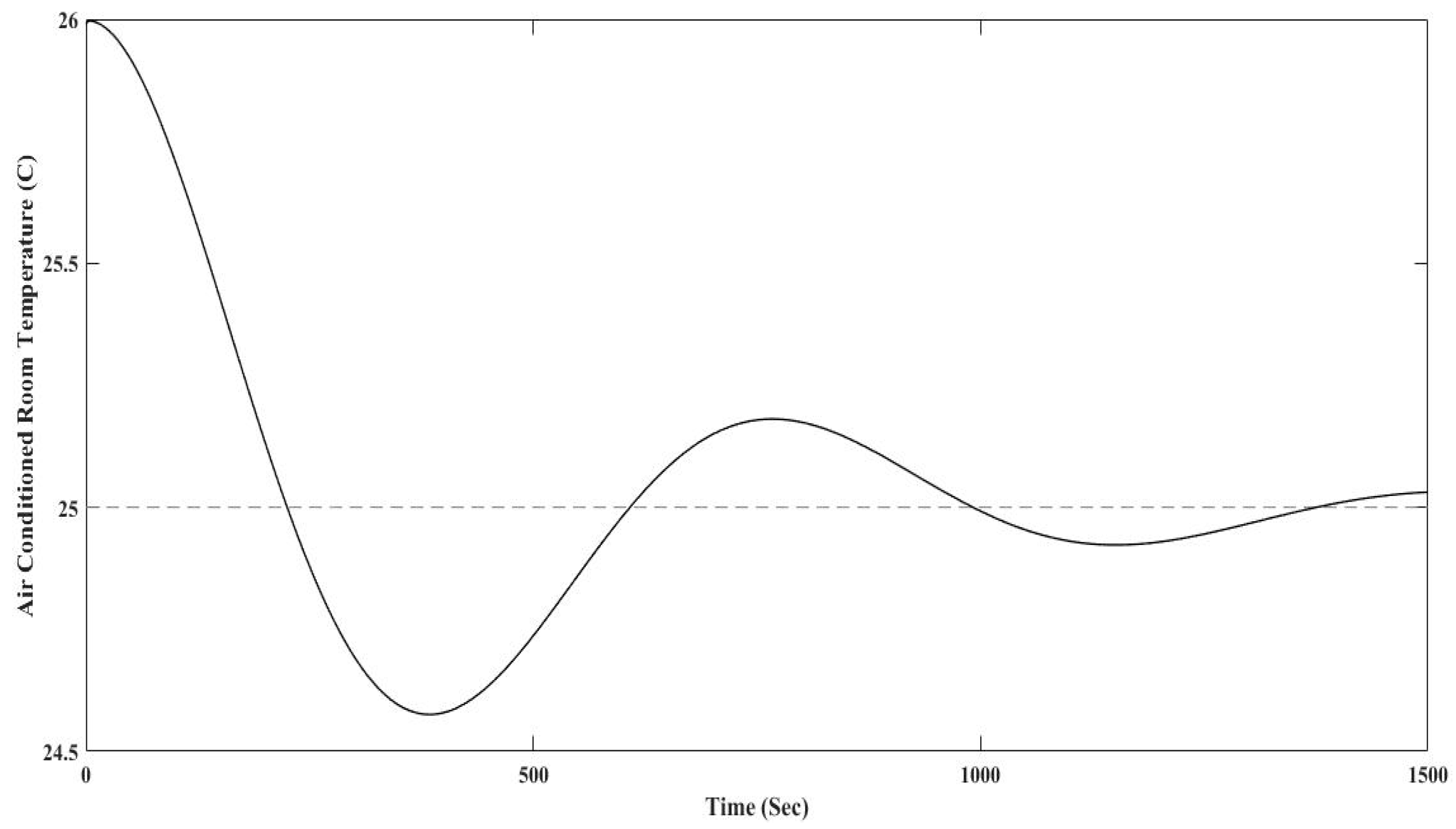
The temperature of the air conditioned room by LQG controller is shown in
Figure 26. The temperature decreased from 26 °C and oscillated around 25 °C in about 1148 s and was maintained. By increasing the compressor speed and flow rate of the fan, the temperature decreased from 26 °C to 25 °C in about 1148 s. The temperature reached the desired set point in 19.13 min with a 2.6% error and the temperature was maintained at the desired set point.
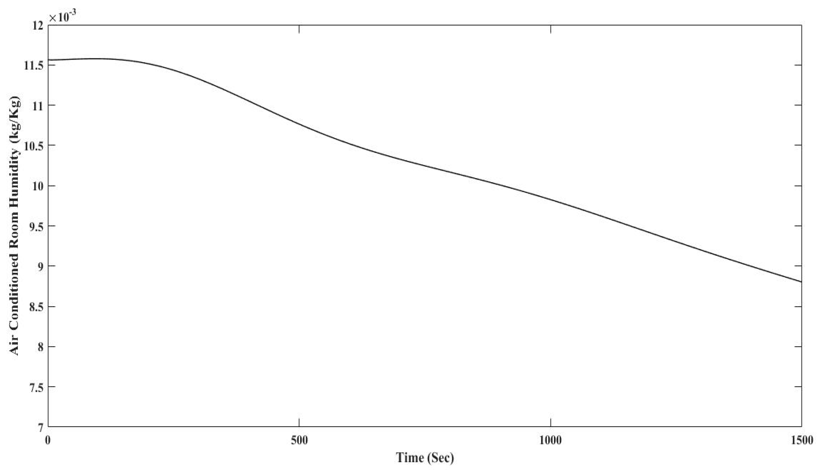
Figure 27 indicates the air-conditioned room humidity established by the LQG controller which decreased from 0.01057 kg/Kg to 0.00901 kg/Kg in about 1342 s and was maintained. By increasing the compressor speed and flow rate of the fan, the humidity of the air-conditioned room decreased from 50% humidity for 26 °C to 46.1% for 25 °C in 22.36 min with 4.8% error from 50% humidity.
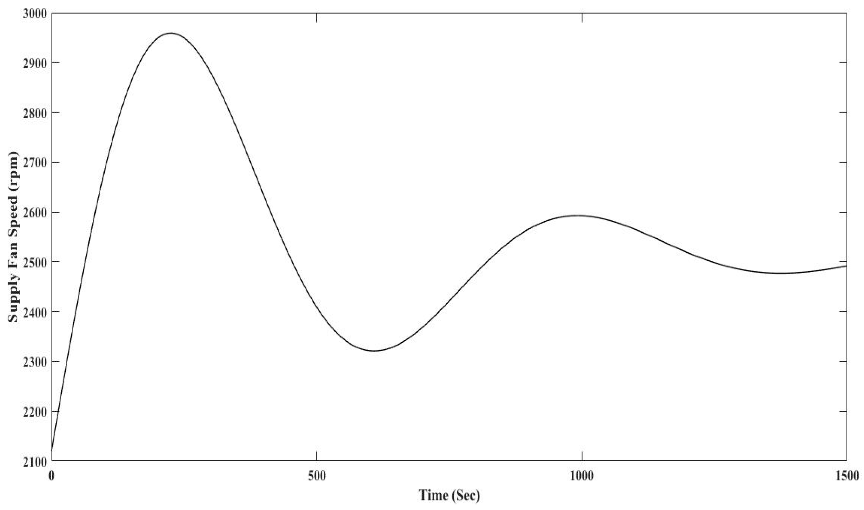
The speed of the supply fan is indicated in
Figure 28. The speed of the fan increased from 2120 rpm to 2595 rpm at 220 s then decreased to 2321 rpm at 609 s and finally reached 2515 rpm at 1204 s and was maintained. When the temperature of the room reached the desired values, the speed of the fan started to decrease until it reached the required speed for keeping the air-conditioned room temperature and humidity at the desired set points. The speed of fan decreased to 2515 rpm at 1204 s and maintained the speed.
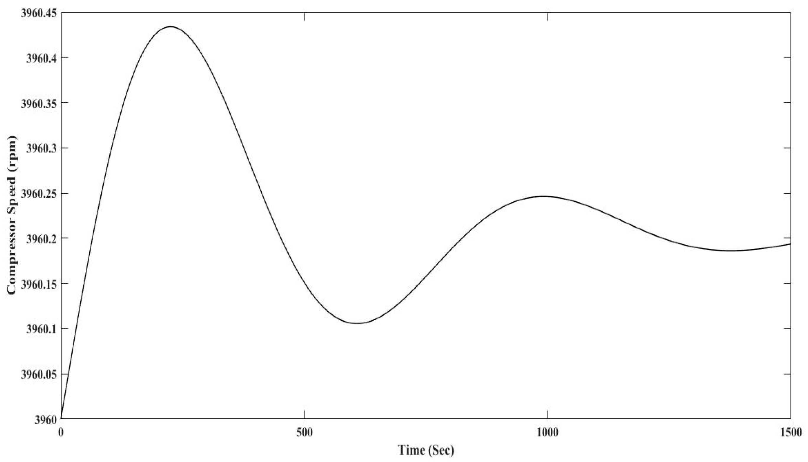
Figure 29 shows the speed of the compressor. To decrease the temperature of the air conditioned room, the compressor speed increased from 3960 rpm to 3960.42 rpm in 223 s, then by declining the air conditioned room temperature to the desired value, the speed of compressor decreased to 3960.1 rpm at 609 s and finally reached to 3960.2 rpm at 1197 s and maintained to keep the air conditioned room temperature and humidity in desired set points.
In 1500 s, the energy usage by compressor is 5.94 × 10⁶ (W) and the energy usage by supply fan is 3.828 × 10⁶ (W). The total energy usage by applying LQG controller is 9.768 × 10⁶ (W). It is clear that compared to the LQG controller, there is 0.216 × 10⁶ (W) reduction in energy usage in 1500 s runtime of the system by applying the GPC-FCM controller. This can be translated into a huge amount of energy savings per year.
In order to compare the performance of both controllers, the performances of the GPC-FCM controller and LQG controller which are applied on the same DX A/C system are compared under the same non-linear conditions by the ISE, IAE, and ITAE performance indexes [
40,
41,
42]. The results are summarized in
Table 3.
Integral Square Error (
ISE)
Integral of the absolute magnitude of error (
IAE)
Integral Time-absolute error (
ITAE)
The parameter y(t) is the measured control output and r(t) is the desired set point value and t is time.
According to the performance indexes results, it is clear that the GPC-FCM controller is able to minimize the performance indexes more than the LQG controller. In other words, the GPC-FCM controller is working better than the LQG controller under the same room conditions. This means that the GPC-FCM controller is more appropriate and applicable in comparison with the previous work on the same system.

 ,
, 


