Deterministic Algorithm for Selective Shunt Active Power Compensators According to IEEE Std. 1459

Abstract

This paper proposes a deterministic algorithm to scale the reference currents of a shunt active power compensator (SAPC) based on IEEE Std. 1459 power decomposition when SAPC maximum output compensating current is going to be exceeded. The selective SAPC is proposed to improve power quality and energy efficiency in power networks by means of the cancelation or reduction of the non-efficient powers (Q₁⁺, S_U1, S_eN). The non-efficient powers can be reduced in six possible sequences according to the priority of compensation. When SAPC maximum output current capacity is exceeded, the proposed algorithm limits the SAPC output compensating currents and the non-efficient currents can only be partially reduced in the power network. The reduction of the non-efficient powers depends on the selected compensation sequence. Experimental results for several compensation sequences demonstrate the appropriate operation of the selective SAPC using the proposed scaling algorithm.

1. Introduction

The existence of non-efficient powers in electrical systems causes increases in line and transformer power losses, lack of stability of the electrical system, voltage asymmetries, distortions in the three-phase power supply, and so on. SAPCs are developed to improve power quality and energy efficiency in the electrical system, providing the load non-efficient currents and avoiding the flow of these currents through the power network. When SAPCs have enough current capacity, non-efficient currents can be completely compensated (global compensation) and the power system operates with the highest power quality standards. Some studies related to the reduction of the non-efficient currents for unbalanced three-phase four-wire systems under non-sinusoidal conditions using the global compensation approach are detailed in [1,2,3,4,5,6,7]. In [7] the authors present a bidirectional front-end converter connected between the mains power system and a general purpose DC bus connecting distributed generators and passive loads. The bidirectional power flow with the mains is achieved by means of fundamental component currents.

In the last decade, the interest in the selective compensation of load non-efficient currents has increased, as it is demonstrated by the number of publications dealing with this topic [8,9,10,11,12,13,14,15,16,17,18,19]. Selective SAPCs contribute to reduce losses in the power networks and at the same time can be used for the dynamic support of the grid following the settings established by the power network managers.

According to IEEE Std. 1459, the non-efficient currents can be decomposed in fundamental and harmonic current terms. Selective SAPCs usually focus on the harmonic currents cancellation, without considering the non-efficient currents demanded by unbalanced and reactive linear loads. Most of the works dealing with harmonic cancellation concern about fast response and harmonic detection [8,9,10]. However, they do not focus on the SAPC rating and overloading issues.

SAPC rating is determined by the maximum instantaneous current that can be delivered. In the case of SAPC overloading condition, the non-efficient currents demanded by loads cannot be completely compensated and the SAPC output currents must be limited or the SAPC must be disconnected. The implementation of a selective SAPC permits to choose the SAPC output compensating currents that avoid SAPC overloading. The most common strategy in selective compensation consists in applying the full or nil compensation of the individual non-efficient current terms, depending on SAPC overloading. With this approach, the operation limits of the components used in the SAPC implementation are not completely achieved and the SAPC does not work at its maximum capabilities [14,15,16,17].

A current limiter combined with a control algorithm is proposed in [14] to avoid SAPC overload. The control is based on a current hysteresis loop limiter. They ensure that the SAPC is not overloaded by means of limiting the instantaneous active and non-active currents injected to the power network. The power theory used for the compensation only distinguishes between active (P) and reactive power (Q), without recognizing harmonics or unbalances as non-efficient power terms.

A priority resolver and a gain scheduler are proposed in [15] to avoid SAPC overloading. The SAPC control performs the decomposition of the load current in active, reactive, harmonic, and negative-sequence fundamental current components. The SAPC control sets gains to adjust the reference currents; nevertheless, the algorithm used to obtain such gains is not detailed. A fixed priority compensation order is also established in [15], with harmonic currents being the first preference, followed by the negative sequence and the reactive current components. Another drawback is related to the use of a three-phase three-wire SAPC, which cannot compensate zero-sequences currents that could exist in power networks.

A three-phase four-wire SAPC is used in [16] to allow zero-sequences currents compensation. The SAPC control includes a priority resolver and a gain scheduler, but they assign a gain equal to zero when no compensation is selected or a gain equal to 1 for the full compensation of the selected current term. Load current is decomposed into the following current terms: fundamental positive active, fundamental positive reactive, fundamental negative-sequence, zero-sequence, and harmonic reactive. Zero-sequence current and harmonic current terms are included in the same expression not being possible a complete selective compensation following IEEE Std. 1459 power decomposition.

A control algorithm for selective grid harmonics and interharmonics compensation that relies only on the measurement of the voltage at the point of common connection of distributed generation units is presented in [17].

A SAPC optimization algorithm based on linear matrix inequalities (LMIs) is proposed in [18], with a power decomposition that is also based on IEEE Std. 1459. The algorithm is implemented in an experimental three-phase four-wire SAPC prototype. A quadratically-constrained quadratic program is solved by means of LMI formulation, which permits obtaining gains for selective compensation when SAPC is overloaded. The main drawback is that the reference currents are calculated on a PC, not being adequate for rapid changes of load current. Another inconvenience is that the current decomposition is done in rectangular coordinates without identifying the different non-efficient components of the load current. Additionally, it operates with root mean square (RMS) phasors, losing waveform information.

This paper deals with the use of a deterministic algorithm for the selective compensation of the load non-efficient currents that a SAPC can compensate when overloading problems arise. The proposed algorithm extends the work presented in [19] by means of the calculation of the scaling factors that, multiplied by the load non-efficient current terms, permit achieving the SAPC maximum capabilities. The SAPC control obtains the SAPC reference compensating currents based on IEEE Std. 1459–2010 [20,21,22]. These currents are scaled using variable factors, avoiding SAPC overloading and permitting the selective compensation to follow an established compensation sequence. The proposed algorithm is deterministic and is based on the information given by the SAPC reference compensating current waveforms. It permits to use all the current capability of the SAPC, achieving the maximum SAPC compensation. The SAPC operation under global compensation mode or selective compensation mode is performed doing the comparison of the maximum instantaneous SAPC output current with the maximum current permitted in the SAPC output. Maximum current in the SAPC output can be limited by the characteristics of the power switches used in the inverter or the passive components in the SAPC output filter.

This paper is organized as follows. In Section 2, SAPC reference currents for the non-efficient power compensation are detailed, ending with the expression proposed for the selective non-efficient current compensation. In Section 3 the algorithm that adjusts the reference currents when the SAPC is overloaded is described. Section 4 shows the experimental results obtained with a SAPC prototype that validates the proposed algorithm. In Section 5, the paper concludes with a summary of the main achievements obtained in the study.

2. SAPC Output Currents for Selective Compensation According to IEEE Std. 1459 under Overloading Conditions

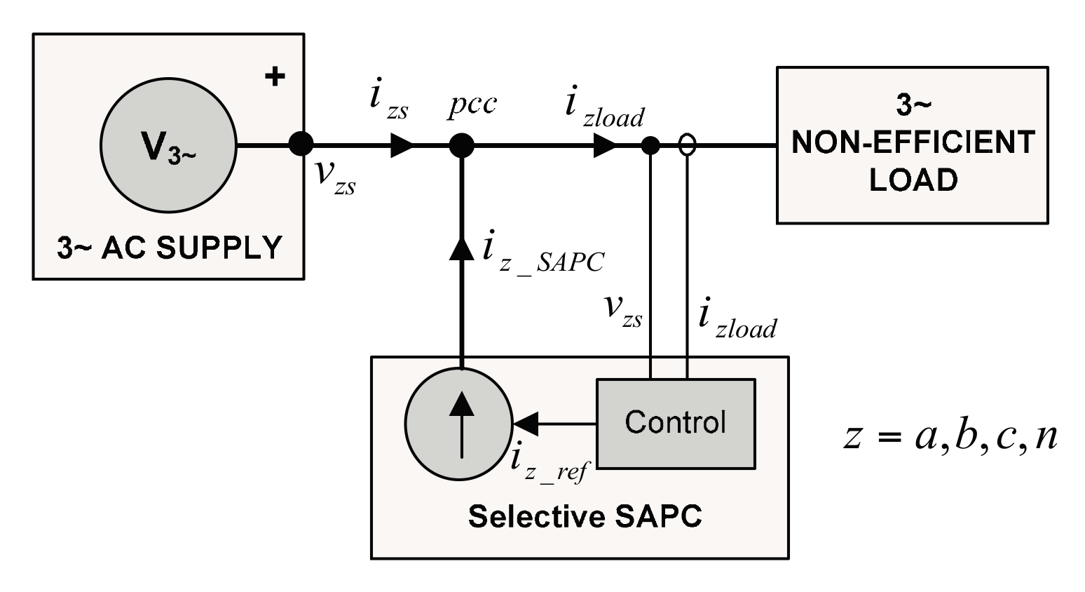
A SAPC is equivalent to a controlled three-phase AC current source, as shown in the block diagram of Figure 1. A current control loop ensures that the currents at the SAPC output, the SAPC compensating currents, are proportional to the reference currents calculated by the SAPC control. The SAPC compensating currents improve the power quality of the electric distribution system upstream the point of common connection (pcc) of load, SAPC, and power network.

The SAPC output currents (i_{z_SAPC}) are calculated from the measurement of the load currents (i_zload) and the supply voltages (v_zs) at the pcc (z = a, b, c). Global compensation is used when the SAPC has enough capacity to compensate all non-efficient powers detailed in [23]: positive-sequence reactive power (Q₁⁺), unbalance power (S_U1), and non-fundamental effective apparent power (S_eN). As indicated in [24], the SAPC output currents for global compensation (i_{z_SAPC_G}) are calculated as follows:

$$i_{z\_SAPC\_G}^{}=i_{zload}-i_{z1load}^{+a}$$

(1)

where $i_{z1load}^{+a}$ are the instantaneous load fundamental positive-sequence active phase currents. These current terms represent the useful currents demanded by the load and are presented in the expression of the fundamental positive-sequence active power (P₁⁺), the unique power term considered efficient [23,25]. The main drawback of a SAPC under overloading condition and using global compensation algorithms is that the SAPC can supply new harmonic components into the power networks, affecting other loads connected in the same distribution system and reducing the power quality indicators.

Selective compensation mode is used when SAPC output current capacity is exceeded. Under this condition, powers Q₁⁺, S_U1, and S_eN can only be partially reduced or some are cancelled while others are still present without modification. The approach used to obtain the reference currents of a selective SAPC based on the non-effective power magnitudes defined in IEEE Std. 1459–2010 was presented in [19]. The approach relates each non-efficient power magnitude with some current terms, allowing the selective compensation of the load non-efficient powers. The SAPC output currents that cancel Q₁⁺ and keep P₁⁺, S_U1, and S_eN unchanged in the supply lines are as follows:

$$i_{zQ1\_SAPC}^{}=i_{z1load}^{+r}$$

(2)

where $i_{z1load}^{+r}$ are the instantaneous load fundamental positive-sequence reactive phase currents and exhibit a phase shift of 90° with respect to v_z1⁺. The fundamental positive-sequence active voltage in phase a (v_a1⁺) is the origin of all phase angles. The SAPC output currents that cancel only S_U1 are calculated as follows:

$$i_{zU1\_SAPC}^{}=i_{z1load}^{-}+i_{z1load}^0$$

(3)

where $i_{z1load}^{-}$ and $i_{z1load}^0$ are the instantaneous fundamental negative- and zero-sequence load currents. These fundamental current terms appear due to the connection of linear unbalanced loads in three-phase four-wire power systems. The SAPC output currents that only cancel S_eN are obtained as follows:

$$i_{zH\_SAPC}^{}=i_{zload}^{}-i_{z1load}^{}$$

(4)

where i_z1load are the instantaneous load fundamental currents while i_{zH_SAPC} only contains the instantaneous non-fundamental currents demanded by non-linear loads. The SAPC output currents that cancel all load non-efficient currents (global compensation mode) can be obtained if Equations (2)–(4) are added up as follows:

$$i_{z\_SAPC\_G}^{}=i_{zQ1\_SAPC}^{}+i_{zU1\_SAPC}^{}+i_{zH\_SAPC}^{}$$

(5)

Equations (1) and (5) yield the same result and can be used to compensate the non-efficient currents demanded by the load. When the SAPC output current capacity is exceeded, the SAPC must be disconnected to avoid its failure or the SAPC output currents must be scaled to avoid SAPC overloading. To adjust the SAPC output currents to a value equal or smaller than the SAPC maximum output current (I_{SAPC_max}), scaling factors K_Q, K_U, and K_H are multiplying in Equation (6) their corresponding current terms. The scaled SAPC output currents (i_{z_SAPC_K}) are calculated as follows:

$$i_{z\_SAPC\_K}^{}=K_Q\cdot i_{zQ1\_SAPC}^{}+K_U\cdot i_{zU1\_SAPC}^{}+K_H\cdot i_{zH\_SAPC}^{}$$

(6)

The SAPC instantaneous output currents (i_{z_SAPC}) must not exceed, at any instant, the maximum SAPC output current (I_{SAPC_max}) to avoid SAPC overloading (I_{SAPC_max} ≥ i_{z_SAPC_K}). The subscript “K” is used to indicate that the SAPC selective mode is used. The algorithm to assign the values of K_Q, K_U, and K_H according to the power compensation sequences and SAPC current capacity is explained in the next section.

3. Calculation of the Scaling Factors in a Selective SAPC

The full cancellation of the load non-efficient powers can be achieved when the SAPC has enough current capacity (I_{SAPC_max} ≥ I_{z_SAPC_G_max}), therefore K_Q = K_U = K_H = 1. When the output current limit in the SAPC is reached, the SAPC can only partially reduce the non-efficient powers demanded by the load. The values of K_Q, K_U, and K_H depend on the selected power compensation sequence, the value of I_{SAPC_max} and the load characteristics. Scaling factors K_Q, K_U, and K_H can vary between “0” (no compensation) and “1” (full compensation). The SAPC output effective power, when operating in the selective mode, is calculated as follows:

$$S_{SAPC}^{}=\sqrt{{\left(Q_{1\_SAPC}^{+}\right)}^2+{\left(S_{U1\_SAPC}^{}\right)}^2+{\left(S_{eN\_SAPC}^{}\right)}^2}$$

(7)

There are six possible compensation sequences (CS), attending to the priority given during the compensation to the three main non-efficient power terms (Q₁⁺, S_U1, and S_eN) recognized in [23]. The priority in the compensation order can be assigned on the basis of importance of power quality defects, power losses in lines and transformers, engineering economic decisions, and, moreover, considering the interests of consumers and utilities.

Table 1. SAPC power compensation sequences.

Compensating Current Priority	CS1	CS2	CS3	CS4	CS5	CS6
iz_comp_1	SeN	SeN	SU1	Q1+	SU1	Q1+
iz_comp_2	SU1	Q1+	SeN	SeN	Q1+	SU1
iz_comp_3	Q1+	SU1	Q1+	SU1	SeN	SeN

shows the six CS, where i_{z_comp_1} correspond to the compensating current terms with the highest priority, i_{z_comp_2} are the second current terms to be compensated, and i_{z_comp_3} correspond to the current terms with the lowest priority. i_{z_comp_1}, i_{z_comp_2}, and i_{z_comp_3} are defined to denote the phase compensating currents without establishing a particular sequence of power compensation between Q₁⁺, S_U1, and S_eN. The corresponding scaling factors are denoted as K₁, K₂, and K₃, respectively. Scaling factors K₁, K₂, and K₃ are defined to allow partial compensation of i_{z_comp_1}, i_{z_comp_2}, and i_{z_comp_3} respectively. For example, CS1 indicates that the first power term to compensate is S_eN, followed by S_U1 and Q₁⁺, Q₁⁺ being the last one to be compensated.

With the use of the CS, Equation (6) can be rewritten as follows:

$$i_{z\_SAPC\_K}^{}=K_1\cdot i_{z\_comp\_1}^{}+K_2\cdot i_{z\_comp\_2}^{}+K_3\cdot i_{z\_comp\_3}^{}$$

(8)

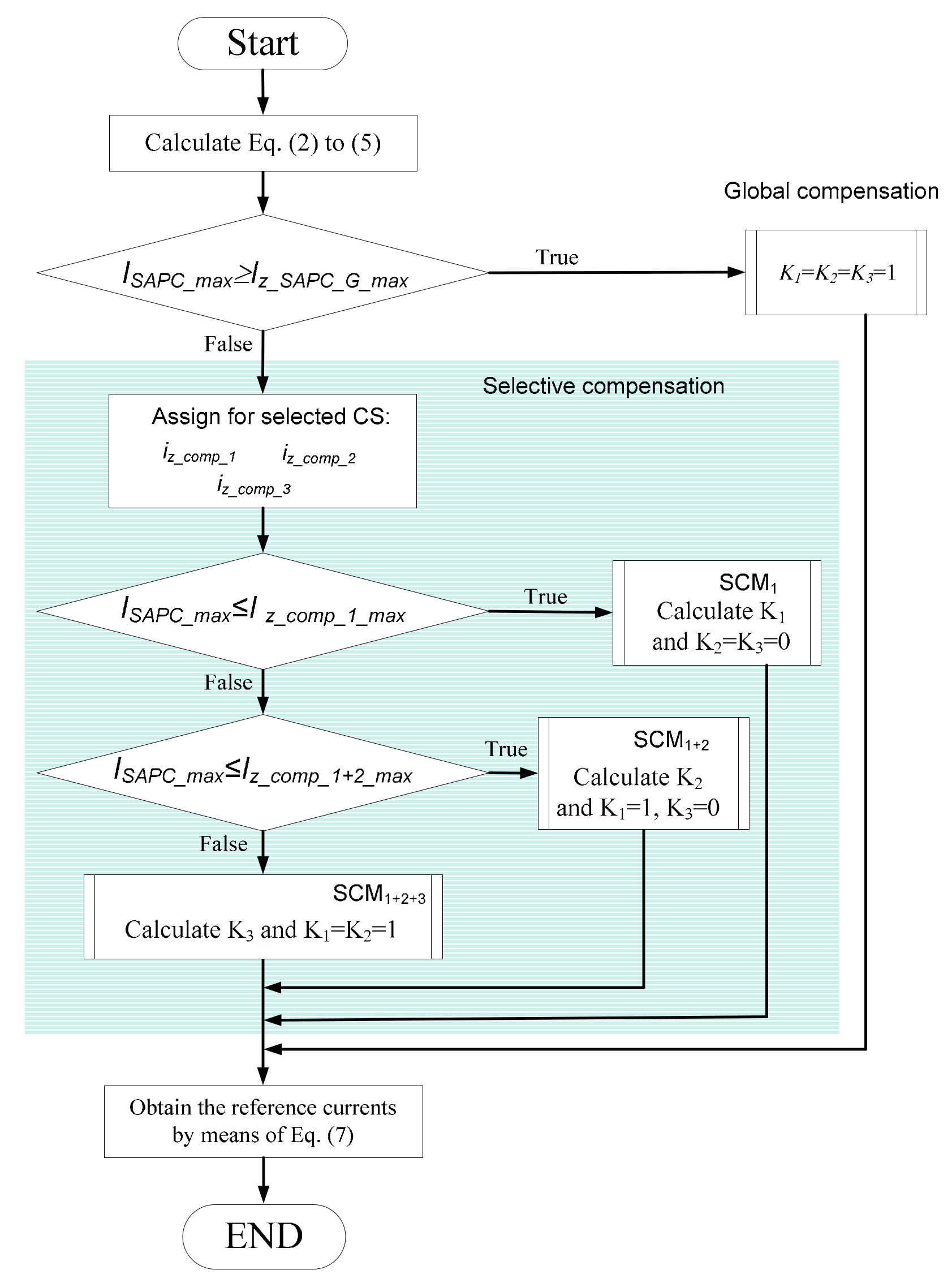
If a global compensation mode is used, i_{z_comp_1}, i_{z_comp_2}, and i_{z_comp_3} are completely compensated and K₁ = K₂ = K₃ = 1. If a selective compensation mode is needed, three situations arise. These three cases are included as software functions in the flowchart of the main algorithm shown in Figure 2, being denoted as selective compensation modes SCM₁, SCM₁₊₂, and SCM₁₊₂₊₃, as appears in the first column in

Table 2. Scale factor assignment.

Operating Mode	iz_comp_1	iz_comp_2	iz_comp_3
Global Comp.	K1 = 1	K2 = 1	K3 = 1
SCM1	0 < K1 ≤ 1	K2 = 0	K3 = 0
SCM1+2	K1 = 1	0 < K2 ≤ 1	K3 = 0
SCM1+2+3	K1 = 1	K2 = 1	0 < K3 ≤ 1

.

The scaling factor of the SAPC output currents must be constant for a complete period of the fundamental current wave to avoid the injection of harmonic current into the power networks. Sub-periodic variable scaling factors cut the waveform and cause new non-fundamental currents in the power network. To avoid an unbalanced compensation, each scaling factor must be unique (the same value for all the phases). Unequal scaling factors asymmetrically modify the reference currents and cause the flow of new unbalanced currents through the power lines.

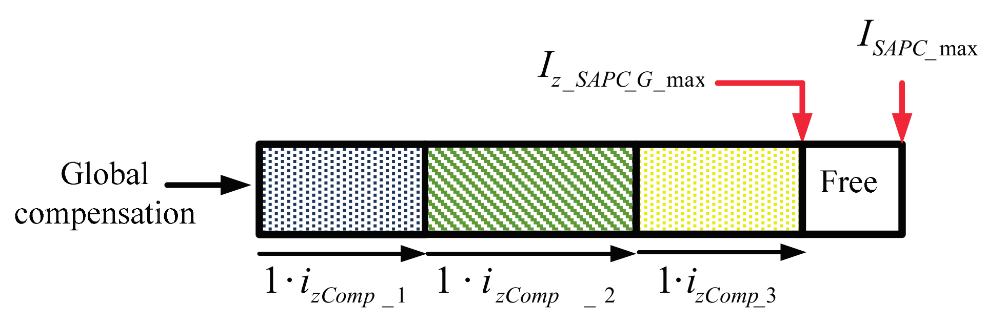
The algorithm used to adjust the SAPC output currents is mainly divided into three comparisons and four subroutines. The result of the comparisons establishes whether the SAPC is operating in the global compensation mode or in one of the three SCM. Each SCM has its corresponding subroutine, which ends in establishing the adequate scaling factors. The algorithm starts calculating the phase currents defined in Equations (2)–(5) during a complete fundamental period. A true answer in the first comparison means that the global compensation is selected since the SAPC has enough capacity to compensate all non-efficient currents without reaching I_{SAPC_max}, as it is represented in Figure 3. Subroutine “Global Compensation” returns the values K₁ = K₂ = K₃ = 1 to the algorithm.

The selective compensation mode is activated when in any phase is verified that I_{SAPC_max} < I_{z_SAPC_G_max} and more comparisons must be done to determine the correct scaling factors. Then, attending to the selected CS, the current terms calculated in Equations (2)–(4) are assigned to the corresponding phase compensating currents (i_{z_comp_*}, where * = 1, 2, 3). The SCM₁ subroutine is executed when the maximum value of i_{z_comp_1} is greater than or equal to I_{SAPC_max} in a complete period of the fundamental current wave. In this case, the full or partial compensation of i_{zComp_1} must be applied (0 < K₁ ≤ 1), while i_{zComp_2} and i_{zComp_3} are not compensated (K₂ = K₃ = 0). SCM₁ returns the correct value of K₁ that permits the partial compensation of the non-efficient current with the highest priority considering the CS selected. The subroutine starts calculating the factors K_z1 as follows:

$$K_{z1}^{}=\frac{I_{SAPC\_\max }}{I_{z\_comp1\_\max }}$$

(9)

The minimum value of K_a1, K_b1, and K_c1 is assigned to K₁, as appears in the following expression.

$$K_1^{}=\begin{array}{c}\\ \min \\ z=a,b,c\end{array}\left(\frac{I_{SAPC\_\max }}{I_{z\_comp1\_\max }}\right)$$

(10)

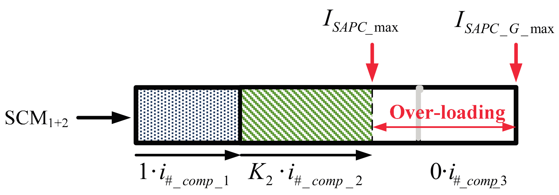
Subroutine SCM₁₊₂ is selected if the SAPC has enough capacity for the complete compensation of i_{z_comp_1} (K₁ = 1), and also has surplus capacity for the partial or complete compensation of i_{z_comp_2} (0 < K₂ ≤ 1). For this situation, i_{z_comp_3} are not compensated (K₃ = 0), as it is showed in Figure 4. SCM₁₊₂ starts calculating the time instant (t_{1+2_max}) when the sum of i_{z_comp_1} and i_{z_comp_2} is maximum (I_{comp_1+2_max}) and determines which of the three phases is limiting the SAPC operation. For the limiting phase, denoted as # (# = {a, b, c}), the values of the currents i_{#_comp_1} and i_{#_comp_2} are calculated at t_{1+2_max}. The following relationships are verified:

$$\begin{array}{l}{i}_{\#\_comp\_1+2}^{}=i_{\#\_comp\_1}^{}+i_{\#\_comp\_2}^{}\\ I_{comp\_1+2\_\max }^{}=\max \left(i_{\#\_comp\_1+2}^{}\left(t_{1+2\_\max }\right)\right)\end{array}$$

(11)

For the three phases, the factor K₂ is calculated as follows:

$$K_2^{}=\frac{I_{SAPC\_\max }-i_{\#\_comp\_1}^{}\left(t_{1+2\_\max }\right)}{i_{\#\_comp\_2}^{}\left(t_{1+2\_\max }\right)}$$

(12)

Subroutine SCM₁₊₂₊₃ is executed if the SAPC has enough capacity for the full compensation of i_{z_comp_1} and i_{z_comp_2} (K₁ = K₂ = 1), but the remaining SAPC capacity only permits the partial compensation of i_{z_comp_3} (0 < K₃ < 1). In this case I_{comp_1+2_max} < I_{SAPC_max} < I_{comp_1+2+3_max}, where I_{comp_1+2+3_max} coincides with the maximum of the global compensation current I_{SAPC_G_max}. The subroutine calculates the time instant (t_{G_max}) where i_{z_SAPC_G} is maximum (I_{SAPC_G_max}) and determines which of the three phases is limiting the SAPC operation. The values of the currents i_{#_comp_1+2} and i_{#_comp_3} are calculated for the phase # that limits the SAPC output current at the instant t_{G_max}, verifying the following expression:

$$\begin{array}{l}{I}_{SAPC\_G\_\max }^{}=i_{\#\_comp\_1+2+3}^{}\left(t_{G\_\max }\right)\\ i_{\#\_comp\_1+2+3}^{}\left(t_{G\_\max }\right)=i_{\#\_comp\_1+2}^{}\left(t_{G\_\max }\right)+i_{\#\_comp\_3}^{}\left(t_{G\_\max }\right)\end{array}$$

(13)

The current available for the compensation of i_{#_comp_3} is calculated as I_{SAPC_max} minus i_{#_comp_1+2}(t_{G_max}), so the value of the factor K₃ for the three phases is calculated as follows:

$$K_3^{}=\frac{I_{SAPC\_\max }-i_{\#\_comp\_1+2}^{}\left(t_{z\_G\_\max }\right)}{i_{\#\_comp\_3}^{}\left(t_{z\_G\_\max }\right)}$$

(14)

Table 2 summarizes the scaling factor used in (8) to obtain the SAPC reference currents.

4. Experimental Results

A three-phase symmetric and fundamental power supply was applied to a three-phase load that includes linear and non-linear parts. During the tests, the load RMS fundamental line to neutral voltages (V_a1, V_b1, and V_c1) were balanced and approximately equal to 125 V.

Table 3. Main voltage magnitudes at pcc (in volts).

Va = 125.46	Vb = 126.82		Vc = 129.26
$\overrightarrow{V_{a1}}=125.44\angle 0°$	$\overrightarrow{V_{b1}}=126.78\angle -120.35°$		$\overrightarrow{V_{c1}}=129.23\angle -239.74°$
$\overrightarrow{V_1^{+}}=127.15\angle -0.03°$	$\overrightarrow{V_1^{-}}=0.82\angle -124.38°$		$\overrightarrow{V_1^0}=1.45\angle 149.23°$
VaH = 2.45	VbH = 3.24		VcH = 3
Ve = 127.19	Ve1 = 127.16		VeH = 2.92
THDVa = 1.95%	THDVb = 2.55%	THDVc = 2.36%	THDeV = 2.30%

shows the main pcc voltage magnitudes (RMS values) calculated applying IEEE Std. 1459. The supply voltages showed, for all performed tests, a distortion lower than 3% and a slight imbalance.

The load used in the test is implemented using an unbalanced linear load in parallel with a balanced three-phase non-linear load. The balanced per-phase non-linear load is built using a single-phase full-bridge diode rectifier with an LC filter and a resistive load (L = 5.0 mH, C = 2.2 mF, R = 100 Ω). The unbalanced linear load is connected from phase terminals (a-b-c) to neutral wire (n) and has the following values:

• Z_{a load} = R_{a load} = 65.9 Ω//L_{a load} = 67.2 mH.
• Z_{b load} = L_{b load} = 67.2 mH (R_{b load} = ∞ Ω).
• Z_{c load} = L_{c load} = 69.7 mH (R_{c load} = ∞ Ω).

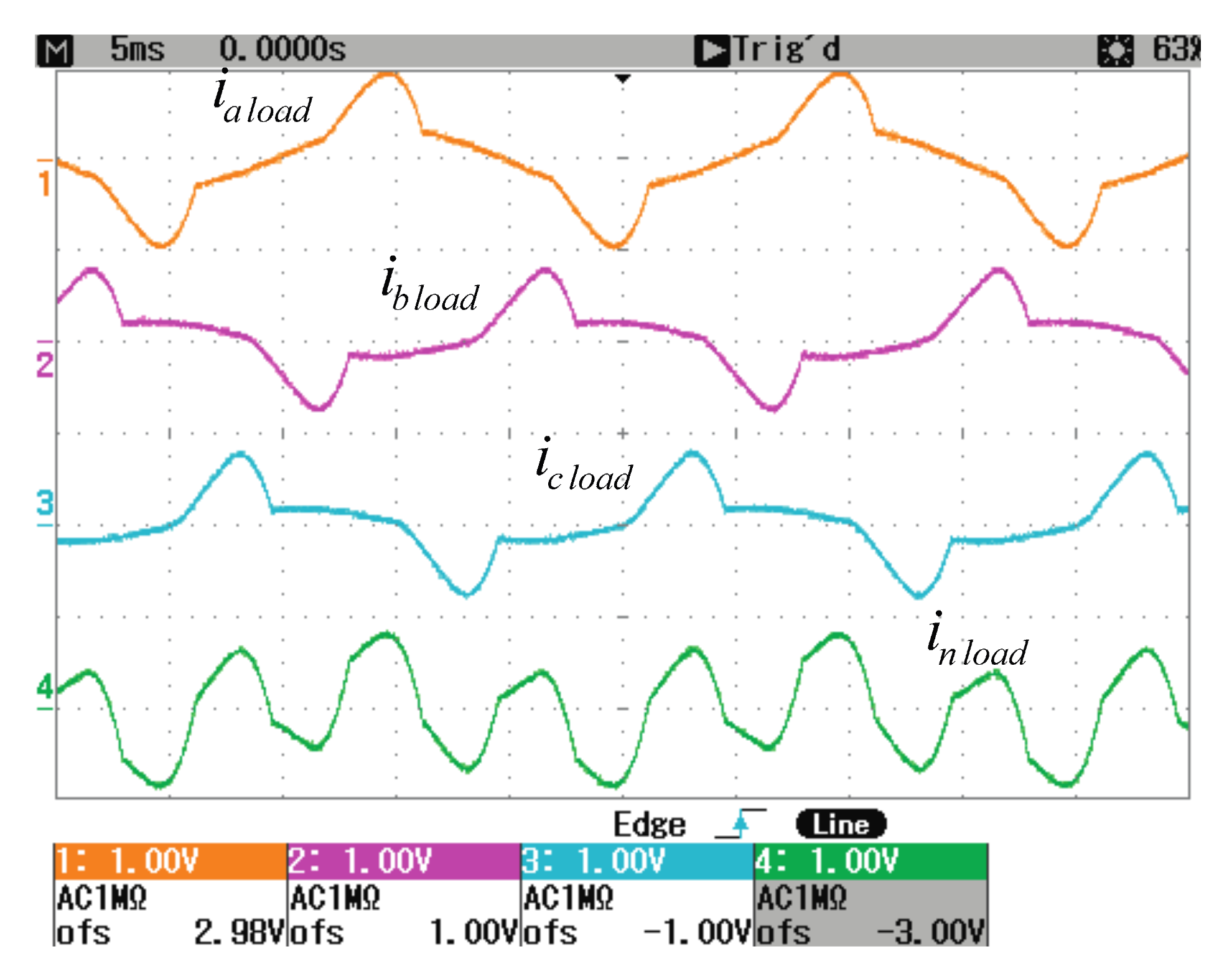
Figure 5 shows the load current waveforms (phases a-b-c and neutral from top to bottom).

Table 4. Main load current magnitudes (in amps).

Ia = 4.83	Ib = 3.54		Ic = 3.52		In = 4.8
$\overrightarrow{I_{a1}}=4.52\angle -28.62°$	$\overrightarrow{I_{b1}}=3.14\angle -166.18°$		$\overrightarrow{I_{c1}}=3.08\angle -283.65°$		$\overrightarrow{I_{n1}}=1.65\angle -2.59°$
$\overrightarrow{I_1^{+}}=3.54\angle -38.07°$		$\overrightarrow{I_1^{-}}=0.63\angle -0.45°$		$\overrightarrow{I_1^0}=0.55\angle 2.59°$
$\overrightarrow{I_{z1load}^{+a}}=2.79\angle 0°$			$\overrightarrow{I_{z1load}^{+r}}=2.18\angle -90°$
IaH = 1.7	IbH = 1.64		IcH = 1.71		InH = 4.51
Ie = 4.01		Ie1 = 3.64		IeH = 1.68
THDIa = 37.6%	THDIb = 52.2%		THDIc = 55.5%		THDeI = 46.1%

summarizes the main load current magnitudes calculated applying IEEE Std. 1459 to the samples acquired with the oscilloscope.

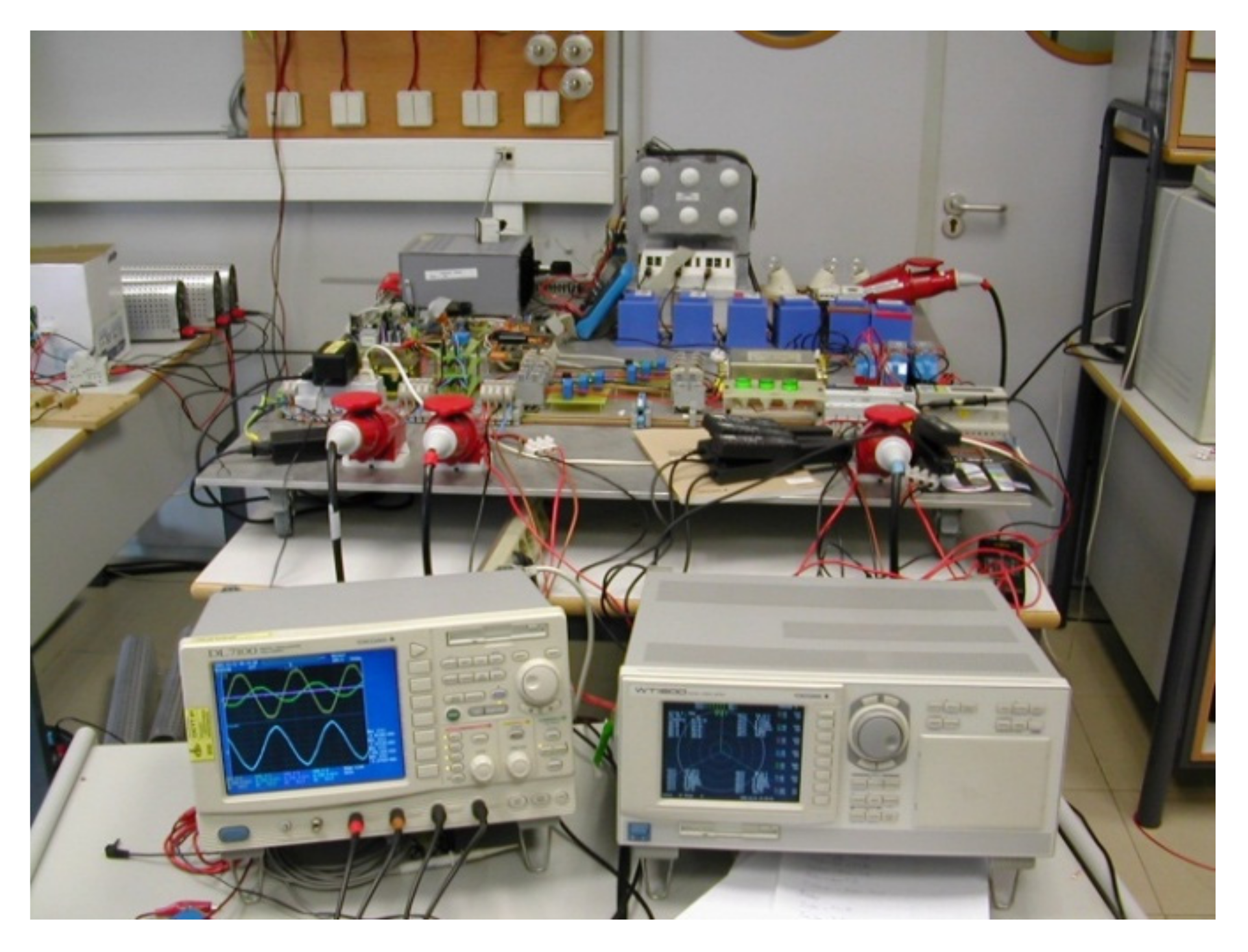
A selective SAPC like the one described in references [21,22,25] is placed between the power network and the load, at the pcc, as showed in Figure 1. The inverter was built using an intelligent power module (IPM SKiiP 342GD120-314CTV). The SAPC control algorithm was implemented on a TMS320F2812 digital signal processor. The availability of reactive components is the main constraint in the construction of the selective SAPC. The SAPC output inductors connected in each phase have L = 6 mH and a maximum RMS current equal to 10 A, limiting the maximum SAPC output apparent power (S_{SAPC_max}) to 3750 VA. The DC bus has a capacitance equal to 7050 μF and was designed to handle up to 800 V. Voltage and current sensors used in the experimental SAPC are LEM LV 25-P and LEM LAH 50-P, respectively. Figure 6 shows the implementation of the prototype.

Due to load characteristics disposed for the experimental tests, the S_{SAPC_max} was limited by the DSP controller to 1125 VA, so the maximum SAPC output compensating current (I_{SAPC_max}) is equal to 4.24 A (equivalent to 3 A_rms). For the load used in the tests the maximum currents obtained with Equations (2)–(5) are the following: I_{zQ1_SAPC_max} = 3.08 A, I_{zU1_SAPC_max} = 1.34 A, I_{zH_SAPC_max} = 3.21 A, and I_{z_SAPC_G_max} = 5.56 A. With these values, SAPC current capacity is reached and the algorithm needs to be executed for adjusting the reference currents.

According to the load and restricted SAPC’s capacity, the six CS detailed in Table 1 are evaluated.

Table 5. Power magnitudes for load and network for the six CS.

	P1+ (W)	Q1+ (var)	SU1 (VA)	SeN (VA)	Se (VA)
Load	1063.49	832.09	483.76	1183.41	1859.53
CS1 (0; 0.55; 1)	1340.86	812.38	206.06	59.22	1582.35
CS2 (0.4; 0; 1)	1348.73	453.11	512.29	67.42	1513.72
CS3 (0; 1; 0.81)	1314.93	818.16	56.27	198.88	1562.41
CS4 (1; 0; 0.67)	1319.68	18.88	507.42	371.71	1462.04
CS5 (1; 1; 0.29)	1304.56	1.14	33.57	848.36	1556.51
CS6 (1; 1; 0.29)	1304.56	1.14	33.57	848.36	1556.51

shows the scaling factors for the six CS and the power magnitudes calculated upstream the pcc following the definitions detailed in [23]. The current scaling factors were calculated by the proposed algorithm considering SAPC capabilities. Values included in the second row correspond to the load without the SAPC operation. The following rows show the values obtained with the six CS. P₁⁺ is increased approximately in 250 W during SAPC operation because SAPC losses are compensated by means of three balanced fundamental positive-sequence active currents supplied by the power network [19]. The non-efficient currents are full, partial, or not compensated according to the scaling factors determined for each CS. Effective apparent power (S_e) is calculated as follows:

$$S_e^{}=\sqrt{{\left(P_1^{+}\right)}^2+{\left(Q_1^{+}\right)}^2+{\left(S_{U1}^{}\right)}^2+{\left(S_{eN}^{}\right)}^2}$$

(15)

Compensation sequence CS4 is the one that produces the minimum S_e at the pcc. CS4 has the following scaling factors: K_Q = 1, K_U = 0, and K_H = 0.67. The application of this scaling factors results in a Q₁⁺ that is almost reduced to zero (18.88 VA), a S_U1 that is not compensated, and a S_eN that is partially reduced from 1183.41 VA to 371.71 VA. The reduction in S_eN is equal to 68.5%, slightly greater than the corresponding scaling factor. This small difference is explained due to minor variations in the pcc characteristics during the measurements that were taken in different moments. The same reason explains the small increase that appears in S_U1 when CS4 is applied or in other cases in which the power term is not compensated (K = 0) but the power term presents some variation. Information provided in Table 5 proves that the inclusion of the proposed algorithm in the control of a SAPC permits the selective compensation of the non-efficient currents and reduces the non-efficient powers according to the selected compensation sequence.

Table 6. SAPC maximum current and SAPC output apparent power.

Compensation Sequences	Ia_max (A)	Ib_max (A)	Ic_max (A)	SSAPC (VA)
CS1	4.22	4.22	4.37	1158.14
CS2	4.22	4.37	4.22	1178.92
CS3	4.37	4.06	4.06	1073.42
CS4	4.38	4.37	4.22	1149.22
CS5	4.22	4.39	4.37	1002.69
CS6	4.22	4.39	4.37	1002.69

shows the per phase SAPC maximum currents (I_{z_SAPC_max}) and the apparent power supplied by the SAPC (S_SAPC) for the six CS. Maximum values are used in Table 6 due to the fact that the scaling factor algorithm uses the maximum values of the corresponding signals. It could be considered that the proposed algorithm works appropriately limiting the SAPC currents to the restricted current (4.24 A) in each phase. I_{SAPC_max} is slightly overcome in some cases (I_{z_SAPC_pk} > 4.24 A), due to the current ripple in the SAPC output current waveforms (on the order of 0.1 A) and the characteristics of the current regulator [22]. The values of S_SAPC for the six CS oscillate around 1125 VA. The small deviation around the maximum value established for S_SAPC capacity is related with the SAPC control, which works with the non-efficient currents instead of the non-efficient power terms.

Table 7. Power network current magnitudes when CS4 is applied (in amps).

Ias = 4.72	Ibs = 2.92		Ics = 2.87		Ins = 2.24
$\overrightarrow{I_{a1s}}=4.69\angle 3.69°$	$\overrightarrow{I_{b1s}}=2.87\angle -117.22°$		$\overrightarrow{I_{c1s}}=2.82\angle -234.81°$		$\overrightarrow{I_{n1s}}=1.74\angle 1.72°$
$\overrightarrow{I_{1s}^{+}}=3.46\angle 3.85°$		$\overrightarrow{I_{1s}^{-}}=0.65\angle 4.62°$		$\overrightarrow{I_{1s}^0}=0.58\angle 1.72°$
$\overrightarrow{I_{z1s}^{+a}}=3.45\angle 0°$			$\overrightarrow{I_{z1s}^{+r}}=0.23\angle 90°$
IaHs = 0.51	IbHs = 0.54		IcHs = 0.54		InHs = 1.41
Ies = 3.61		Ie1s = 3.57		IeHs = 0.53
THDIas = 10.9%	THDIbs = 18.8%		THDIcs = 19.2%		THDeIs = 14.8%

shows the currents in the power network (upstream the pcc) when SACP control is applying CS4. The benefits obtained with the proposed selective SAPC operation can be seen if the results included in Table 7 are compared with the corresponding values in the load, detailed in Table 4.

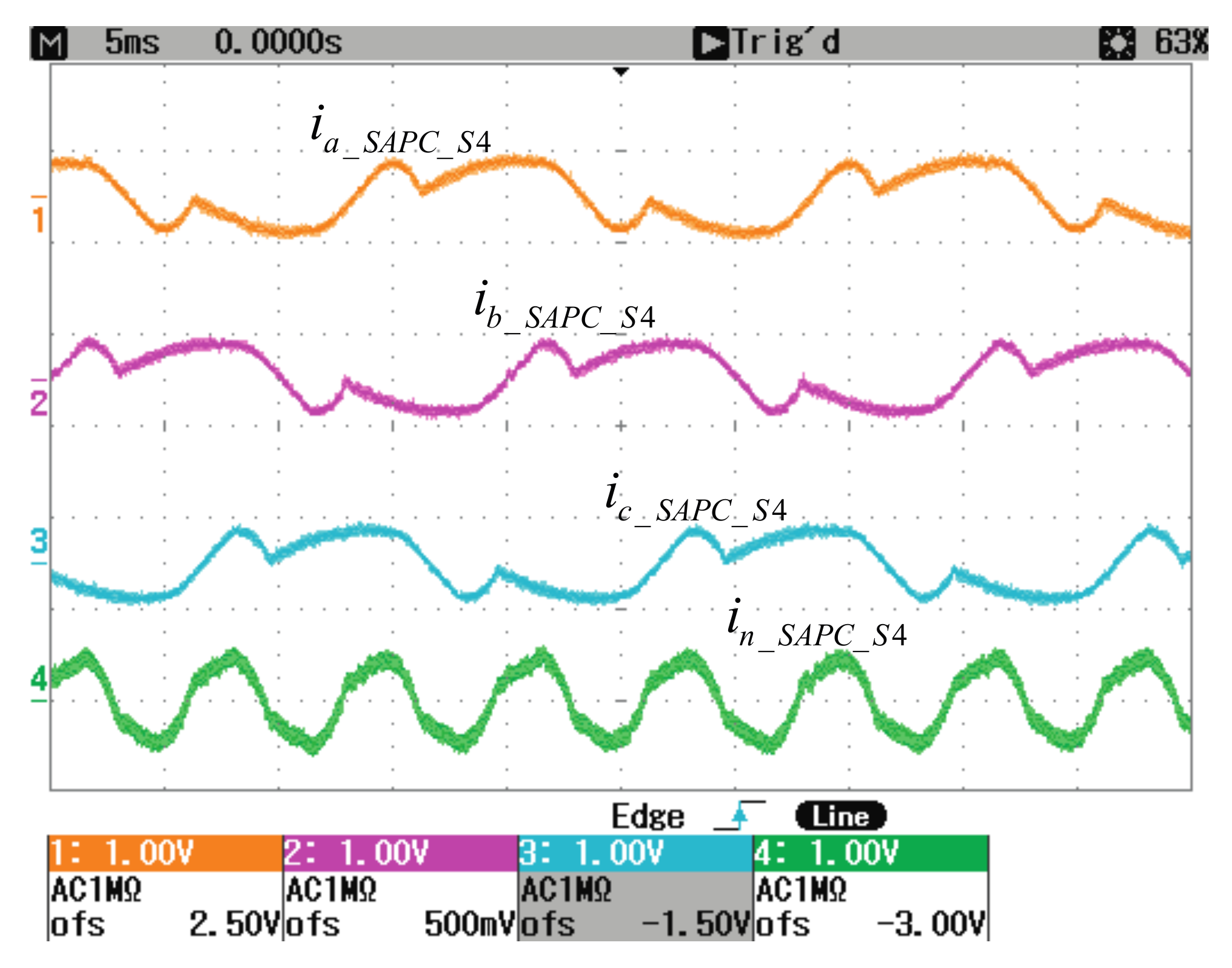
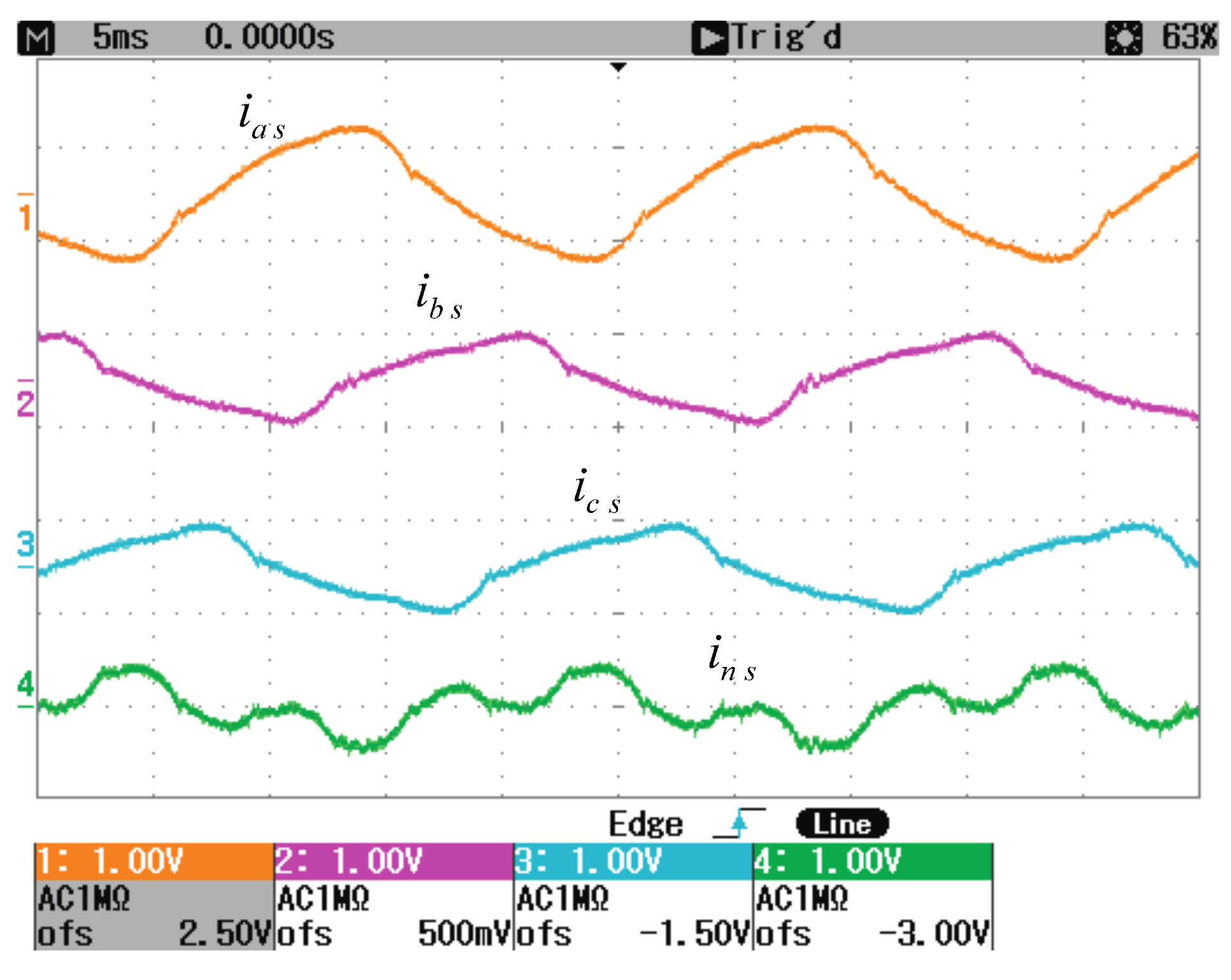
In order to show the algorithm effectiveness, the SAPC output currents and the power network currents for CS4 are shown in Figure 7 and Figure 8, respectively.

For CS4 the SAPC generates the compensating currents for reducing the reactive and distortion currents demanded by the load ($i_{z1\_SAPC}^{+r}$ and i_{zH_SAPC}). The load current term $i_{z1load}^{+r}$ is completely supplied by the SAPC since K_Q = 1, producing the reduction of $I_{z1load}^{+r}$ from 2.18 A to 0.23 A (a reduction of 89.4%). The current i_{zH_SAPC} is partially injected to the pcc since K_H = 0.67, producing the decrease of I_eH from 1.68 A to 0.53 A (a reduction of 68.4%). The current i_{zU1_SAPC} is not compensated since K_U = 0, as it can be seen in the values of I₁⁻ and I₁° that keep similar values as in Table 4 (before compensation) and Table 7 (with CS4 compensation). After compensation, the effective current I_e is reduced from 4 A to 3.6 A. The reduction in the fundamental effective current I_e1 due to the cancelation of $i_{z1load}^{+r}$ is small (from 3.64 A to 3.57 A) since the other fundamental current terms are still present in the load current ($i_{z1load}^{+a}$, $i_{z1load}^{-}$, and $i_{z1load}^0$). The neutral current (I_n) is also reduced from 4.8 A to 2.2 A (a reduction of 54%) due to the reduction of some zero-sequence harmonic currents that can be seen in bottom plot in Figure 5 (load) and Figure 8 (upstream pcc). The harmonic neutral current (I_nH) decreases by 68.8%, varying from 4.5 A to 1.4 A due to K_H = 0.67 for CS4 case. The effect of the SAPC operation is also seen in the THD_i values. Minimum load THD_i is around 37% while with the CS4 selective SAPC operation and they change to values between 10.9% and 19.2%. If a higher decrease in the values of THD_i is desired, CS1 or CS2 must be selected, since both prioritize the cancelation of the harmonic current terms while, in CS4, the SAPC only partially reduces these currents. For the sake of shortness, only values of THD_i are given for CS1: THD_Ia = 1.99%, THD_Ib = 1.99%, THD_Ic = 2.28%, and THD_eI = 1.99%. These values demonstrate how the selective SAPC can be used to reduce the load THD_i to high power quality levels.

5. Conclusions

Based on the analysis of the load instantaneous non-efficient current waveforms, a deterministic algorithm is proposed to avoid the SAPC overloading that appears when load non-efficient currents are greater than the maximum SAPC current capability. The proposed algorithm improves common ON/OFF selective SAPCs in which scaling factors are only 0 or 1. Load non-efficient currents compensated by the SAPC operation are defined considering the first decomposition proposed in IEEE STD. 1459 for the non-efficient powers, including Q₁⁺, S_U1, and S_eN. Three scaling factors (K_Q, K_U, and K_H) are used to reduce the current terms related with Q₁⁺, S_U1, and S_eN. The proposed algorithm permits to obtain the scaling factors that limit the SAPC output currents for the six sequences of current compensation (CS1 to CS6). Each CS gives different priorities to the non-efficient current terms. The values of the scaling factors can vary between 0 and 1. The final value of the scaling factors is determined considering the selected power compensation sequence, the maximum SAPC output current and the load characteristics.

The experimental results included in the paper for the six CS showed the effectiveness of the proposed algorithm. The corresponding scaling factor for the six CS are calculated by the proposed algorithm and applied to the SAPC control. The main current parameters are measured in the power network and compared with the values required by the load. In all cases, the apparent power supplied by the SAPC is around the value of 1125 VA established as a SAPC limit. Results obtained for CS4 are detailed, including current magnitudes and THD_i upstream the pcc. CS4 is selected for being the CS that most reduces the effective power in the power network (S_e is reduced to 1462.04 VA for CS4). Waveforms and magnitudes of the SAPC output and the power network currents are included, demonstrating the correct behavior of the current controller during the operation of the SAPC in the selective mode. The reduction in the non-efficient currents that are flowing in the power networks during the selective SAPC operation agrees with the priorities established in CS4 and the values calculated for the scaling factors. Selecting the corresponding CS, other quality indices can be improved, as it is demonstrated with the small THD_i values (around 2%) obtained when CS1 is selected.

Experimental results demonstrate that the algorithm calculates the scaling factors for any sequence of current compensation. According to the selected CS, the SAPC delivers to the load all, part, or none of the non-efficient current terms. The effectiveness of the algorithm has been experimentally verified for the six CS, showing a direct relationship between the current scaling factor and the compensated non-efficient powers (for CS4 scaling factors are K_Q = 1, K_U = 0, and K_H = 0.67; this yields to the reduction of Q₁⁺ almost to zero, S_U1 is not compensated, and S_eN is partially reduced from 1183.41 VA to 371.71 VA). The inclusion of the deterministic algorithm permits the selective SAPC operation at its maximum capabilities, CS4 most reduces the apparent power in the network and at the same time use adequately the apparent power available (S_SAPC = 1149.22 VA). The proposed algorithm can also be used for other current decompositions: individual harmonics, negative-sequence currents, zero-sequence currents, etc.