Wind Power Ramp Events Prediction with Hybrid Machine Learning Regression Techniques and Reanalysis Data

Abstract

Wind Power Ramp Events (WPREs) are large fluctuations of wind power in a short time interval, which lead to strong, undesirable variations in the electric power produced by a wind farm. Its accurate prediction is important in the effort of efficiently integrating wind energy in the electric system, without affecting considerably its stability, robustness and resilience. In this paper, we tackle the problem of predicting WPREs by applying Machine Learning (ML) regression techniques. Our approach consists of using variables from atmospheric reanalysis data as predictive inputs for the learning machine, which opens the possibility of hybridizing numerical-physical weather models with ML techniques for WPREs prediction in real systems. Specifically, we have explored the feasibility of a number of state-of-the-art ML regression techniques, such as support vector regression, artificial neural networks (multi-layer perceptrons and extreme learning machines) and Gaussian processes to solve the problem. Furthermore, the ERA-Interim reanalysis from the European Center for Medium-Range Weather Forecasts is the one used in this paper because of its accuracy and high resolution (in both spatial and temporal domains). Aiming at validating the feasibility of our predicting approach, we have carried out an extensive experimental work using real data from three wind farms in Spain, discussing the performance of the different ML regression tested in this wind power ramp event prediction problem.

1. Introduction

1.1. Motivation

Wind power is currently one of the most important renewable energies in the world [1] in terms of penetration in the electric power system [2,3], economic impact and annual growth rate [4], both onshore [5] and offshore [6]. Electric power generation is usually carried out in large wind farms [7,8] far from urban centers [9,10], though, in the last few years, urban wind power generation is also gaining impulse [11], including its use in smart grids [12].

The counterpart of the benefits associated with the flourishing of wind energy throughout the world—mainly the reduction of CO${}_2$ emission, one of the causes of global warming [13] and climate change [14]—are problems related not only to the maintenance and management of wind farm facilities, but also to those of power grids. Regarding this, one of the most important problems yet to be solved is the efficient integration [15] of an increasing number of wind energy generators in both the distribution and transmission power grids, which are becoming increasingly complex [16,17]. Such an intrinsically complex nature of power grids is further increased because of the inherent stochastic nature of wind energy [18] that, depending on the weather conditions, can lead to intermittent generation [18]. This can affect the stability, robustness and resilience [16,17] of electric power grids. A useful discussion of the technical differences between these interrelated, but distinct concepts can be found in [17].

Aiming at preserving grid stability in a scenario with a high percentage of intermittent renewable sources—not only wind energy [6], but also photovoltaic [19] and wave [20] energies—power grids need to be made more flexible [21]. In this effort, the emerging technologies associated with smart grids [12] and micro-grids [22] can be used to mitigate wind power intermittency. An illustrative, very recent proposal in this respect consists of increasing the penetration of Vehicle-to-Grid (V2G) technologies [23] to use the batteries of idle Electric Vehicles (EV) as power storage units [24], absorbing peaks of intermittent overproduction.

Wind power intermittency and its influence on power grids’ stability and performance are the main reasons why Wind Power Forecasting (WPF) [25,26] is a key factor to improve its integration without unbalancing the rest of the grid components. Among the different issues in wind power prediction, one of the most significant is the existence of Wind Power Ramp Events (WPREs). WPREs consist of large fluctuations of wind power in a short period of time, leading to a significant increasing or decreasing of the electric power generated in a wind farm [27,28].

The field of scientific research in WPREs’ prediction (or forecasting) [29] is a relatively recent topic driven by the need for improving the management of quick and large variations in wind power output, particularly in the aforementioned context of power grids with high renewable penetration [30]. A useful review of different WPREs’ definitions (in which there does not seem to be a clear consensus) and their types (increasing or decreasing, depending on the WPRE definition) can be found in [31]. Among them, WPREs’ severity is one of the important issues. Up and down WPREs can exhibit different fluctuating levels of severity, although down WPREs are usually more critical than up WPREs because of the availability of reserves [27]. WPREs are usually caused by specific meteorological processes—basically, crossing fronts [32] and fast changes in the local wind direction—and they involve at several scales (synoptic [33], mesoscale [34] and microscale). Surprisingly, it has been found recently that very large offshore farms, clustered together, can also generate large WPREs on time scales of less than 6 h [35]. This gives an idea of the complexity of the WPRE phenomenon.

WPREs’ prediction is not only important for power grid operators, but also for wind farm owners. In fact, the occurrence of WPREs in wind farms is critical not only because of the aforementioned undesired variations of power, but also due to their potential harmful effects in wind turbines, which leads to an increase of management costs associated with these facilities [36]. Regarding this, the accurate prediction of WPREs has been reported as an effective method to mitigate the economic impact of these events in wind generation power plants [28,36].

According to [36,37], the prediction of WPREs and their influence on electricity generation and grid stability have been recently tackled by using two major families of techniques: (1) “physical-based” models (or numerical approaches aiming to tackle the complexity of the physical equations, which rule the atmosphere to obtain a prediction); and (2) statistical approaches (usually data-driven models to obtain predictions). The first group of techniques, the physical-based approaches, include a set of equations that rules the atmospheric processes and their evolution over time and, because of their complexity and nonlinearity, are tackled by means of numerical methods. The second group of WRPE predicting techniques, the statistical approaches, are data-driven methods that are based on wind time series and include a variety of techniques ranging from conventional approaches—for instance, Autoregressive-Moving-Average (ARMA)—to Computational Intelligence (CI) approaches [38]. These are physics-inspired meta-heuristics [38] able to find approximate solutions to complex problems that otherwise could not be solved or would require very long computational time. They include, among others, three groups of bio-inspired techniques such as Evolutionary Computation (EC) [39], Neural Computation (NC) [40] and Fuzzy Computation (FC) [41]. An introduction to the main concepts of bio-inspired CI techniques in energy applications can be found in [20,42]. Examples of NC are Neural Networks (NNs), which are ML algorithms able to learn after training and validation processes. Although it will be shown in more detail in our bibliographic review in Section 2, most of the research works focus on WPREs’ forecast by using either numerical-physical models or statistical approaches, but only a few combine both, mainly focused on WPREs’ classification, but not on prediction.

1.2. Purpose and Contributions

The purpose of this work is to explore the feasibility of a novel hybrid WPRE prediction framework (proposed in this paper), which merges parts of numerical-physical models with state-of-the-art statistical approaches. Specifically, our work presents a system for WPRE prediction based on ML regression techniques, in which the predictive variables are obtained from the ERA-Interim reanalysis data. Reanalysis is a methodology that consists of combining past observations with a modern meteorological forecast physical model aiming at producing regular gridded datasets of many atmospheric variables, with a temporal resolution of a few hours. ERA-Interim represents a pivotal commitment by the European Centre for Medium-Range Weather Forecasts (ECMWF) to produce a reanalysis by including accurate physical atmospheric models and assimilation system. Among the ML regression techniques, we have tested NNs—Multi-Layer Perceptrons (MLPs) and Extreme Learning Machines (ELMs)— Support Vector machines for Regression (SVR) and Gaussian Processes for Regression (GPR). All the algorithm codes have been obtained by public implementations available on the Internet.

When we use the term “hybrid algorithms”, we mean that our proposal combines data from numerical-physical methods (reanalysis, in this case) with ML approaches (specifically, regressors). Regarding what we have called the hybrid approach, there are two points to note. The first one is that it would be possible to adapt the proposed regression techniques to operate with alternative data (not coming from numerical methods, reanalysis, in this paper). The second one, which is the main novelty of our work, is that we prove that the use of data from numerical-physical methods could help achieve valuable prediction of WPREs in wind farms.

The contributions of our work are:

• The use of regression techniques in this kind of problem since, up until now, the majority of WPRE prediction frameworks have been based on classification approaches, as will be shown in the literature review in Section 2.
• The use of direct reanalysis data as predictive variables of the ML regression techniques. As will be shown, this is because the direct application of regression algorithms makes unnecessary the use of some pre-processing algorithms, which are necessary in other approaches [43,44]. Note that the classification problems associated with WPREs are usually highly unbalanced, which makes it difficult to put into practice high-performance classification techniques without having to use specific over-sampling or similar techniques [43,44].
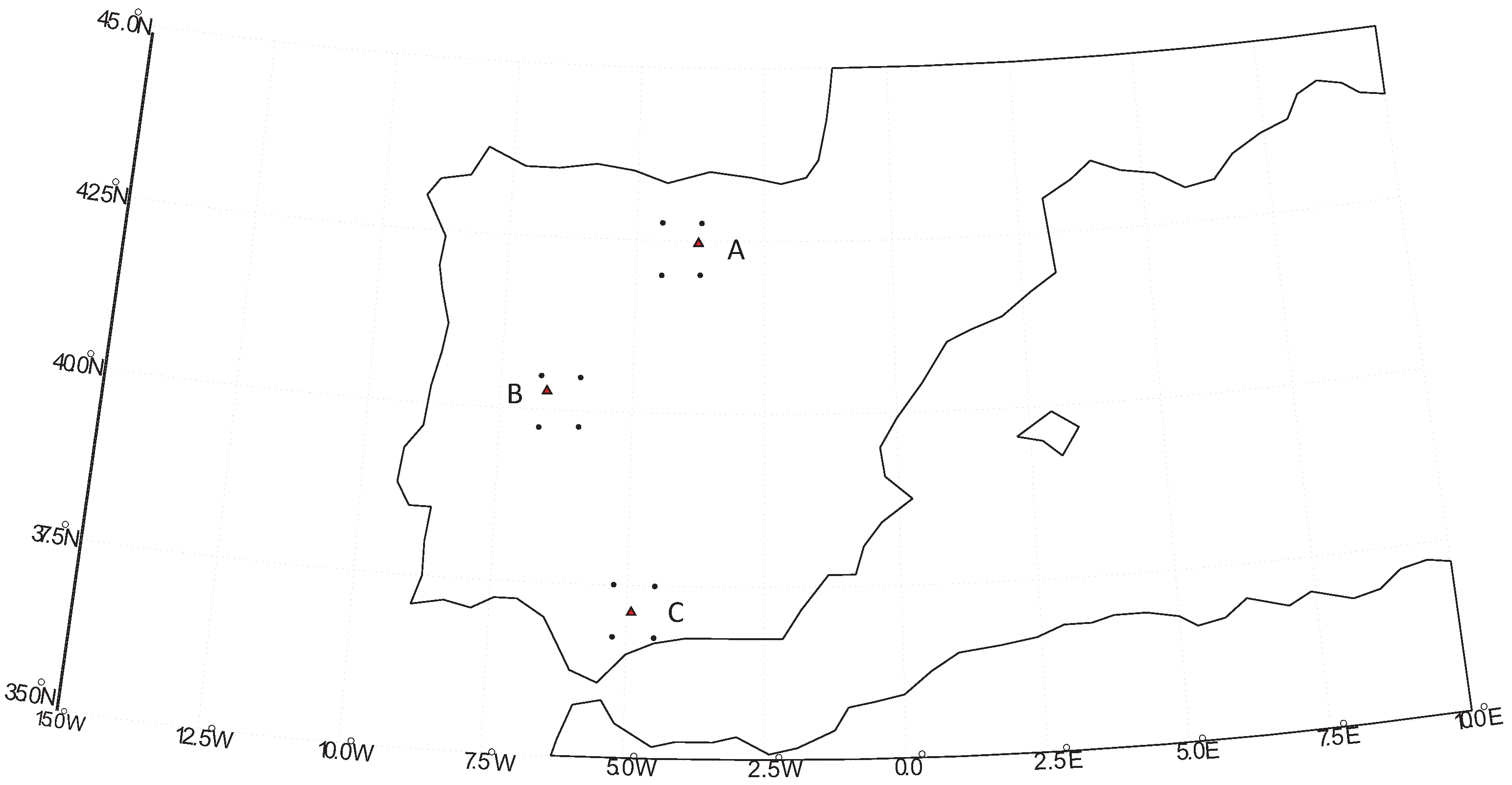
• The performance of the proposed system has been tested using real data from three different wind farms in Spain.

1.3. Practical Perspectives

Section 1.1 has motivated the need for developing novel, more accurate WPRE prediction tools and has illustrated the possible practical application. Going deeper into this regard, WPREs’ prediction can have different goals and practical perspectives depending on the company that needs to use it. Such enterprises are wind power farm owners, utility companies and Independent System Operators (ISOs) [45]. In particular, for ISOs, the ability to predict abrupt changes in wind power generation is one of their major concerns [27].

In this context, our novel hybrid WPRE prediction framework, which combines parts of numerical-physical models and state-of-the-art statistical ML regressors, could help the aforementioned companies improve their WPRE forecasts, aiming at better integration of the wind farms in the power grid (in the case of utility companies and independent system operators) or reducing the damage in turbines (for wind power farms owners).

1.4. Paper Organization

The rest of the paper is organized as follows. Section 2 reviews the state-of-the-art, showing the scientific novelty of our proposal and its practical importance. Section 3 states the problem definition we tackle in this paper, in which the WPRE prediction is formulated as a regression task. Section 4 presents the data and predictive variables involved in our proposal. In Section 5, we describe the main ML regression techniques we have tested to solve the WPRE prediction problem. In turn, Section 6 shows the experimental work we have carried out, these results being obtained by the different tested algorithms in three WPRE prediction problems located at three distinct wind farms in Spain. Section 7 completes the paper by giving some final concluding remarks on the work carried out.

For the sake of clarity,

Table 1. List of acronyms used throughout this research article.

Acronym	Meaning
ANN	Artificial Neural Network
ARMA	Autoregressive Moving Average
CI	Computational Intelligence
CDF	Computational Fluid Dynamics
EA	Evolutionary Algorithm
EC	Evolutionary Computation
ECMWF	European Centre for Medium-Range Weather Forecasts
ELM	Extreme Learning Machine
FC	Fuzzy Computation
GCM	Global Circulation Model
GP	Gaussian Process
GPR	Gaussian Processes for Regression
L1-SVR	L1 Support Vector Regression
MAE	Mean Absolute Error
ML	Machine Learning
MLP	Multi-Layer Perceptrons
NC	Neural Computation
NN	Neural Network
NWM	Numerical Weather Model
NWP	Numerical Weather Prediction
PCA	Principal Component Analysis
RBF	Radial-Basis Function
RC	Reservoir Computing
RMSE	Root Mean Square Error
SAF	Sigmoid Activation Function
SDA	Swinging Door Algorithm
SVM	Support Vector Machine
SVR	Support Vector (machine for) Regression
V2G	Vehicle-to-Grid
WEST	Wind Energy Study of Territory
WPF	Wind Power Forecasting
WPREs	Wind Power Ramp Events
WRF	Weather Research and Forecasting

lists the acronyms used in this paper.

2. Related Work

As mentioned before, according to [36], the prediction of WPREs is usually tackled by means of two groups of methods: numerical-physical models and statistical approaches. Section 2.1 and Section 2.2 review, respectively, the physical-based and statistical approaches, while Section 2.3 discusses the novelty of our proposal, once the literature has been analyzed.

2.1. Physical-Based Models

Physical-based methods take into account both spatial and temporal factors in the framework of the fluid dynamics of the atmosphere [46,47], which include a set of equations that models the atmospheric processes and how the atmosphere evolves with time [48]. The equations that model the motion on the atmosphere (primitive equations) are Newton’s second law of motion (momentum conservation), the first law of thermodynamics (energy conservation), the continuity equation (mass conservation), the equation of state and the equation of water conservation [48]. As mentioned before, modeling atmospheric processes is so complex that, in fact, the aforementioned equations are simplified models of the actual physical atmospheric processes.

Additionally, and because of their non-linearity, a feasible way to solve this problem consists of using numerical models and methods, leading to the so-called Numerical Weather Prediction (NWP) models [48,49,50,51]. To put it simply, in an NWP model, the prediction of future states of the atmosphere is made by numerically modeling the dynamics and other physical processes of the atmosphere. The NWP model predictions are initialized from analyses, which represent the observed state of the atmosphere, on a three-dimensional grid, by combining observational data with an earlier prediction [49,50,51]. Enhancements of NWPs can be done by including some physical aspects of the terrain such as the roughness, orography and obstacles [52]. This is usually carried out by using Computational Fluid Dynamics (CDF), which allows for accurately computing the wind field at the farm location considering the terrain [52]. For further details about wind forecasting using NWP methods, the interested reader is referred to [48,52,53]. Within the field of application of wind energy, NWP models are able to provide, relatively quickly, wind data with high spatial and temporal resolutions. They are able to provide forecasts ranging from the next few hours up to several days ahead [49,50,51].

As a subset of the NWP techniques to predict wind, there are some particular works, specifically focused on WPREs prediction in wind farms, which will be discussed in the following paragraphs for the sake of clarity.

To begin the discussion, it is convenient to start with the recent work [54], which is an illustrative review of state-of-the-art physical models to predict WPREs. In particular, it proposes novel tools and metrics to evaluate and compare different NWP models. The evaluation of a conventional wind power forecasting methodology based on the combination of two Numerical Weather Models (NWMs) has been carried out in [49]. Specifically, the models BoMMesoLAPS (a Limited Area Model with high resolution of 12.5 km) and the Danish Wind Power Prediction Tool (applied to the output of the BoM) have been tested in a problem of WPRE prediction, in time horizons between 19 and 42 h ahead. In [55], NWMs have also been applied to the prediction of WPREs in wind farms. The proposed methodology includes a transformation of the wind speed at each grid point to an equivalent value that represents the surface roughness and terrain at the wind farm area. This modification of the NWM outputs has been found to achieve improvements in WPRE prediction when compared to the raw NWM data. In [56], an NWM has been used to reduce the forecasting error in the detection of up-ramps and down-ramps with uncertain staring times. The results obtained are mainly based on the improvement of the NWM, which is a hard problem itself.

An important point common to the revised papers is that winds computed by NWP models suffer from non-negligible deviations when compared to real wind measurements. This is basically because NWP models may have problems in representing local terrain characteristics (roughness and topography) with sufficient precision and in resolving medium/small-scale meteorological phenomena. These disadvantages can appreciably affect the accuracy of their wind simulations and, consequently, their energy production forecasting [48,57]. Reanalyses and analyses combine those data modeled by NWP methods with atmospheric and oceanic measurements. However, in some cases (such as local offshore wind energy prediction) [57], these approaches have coarse spatial resolutions (50–250 km), which make it difficult to accurately characterize local wind regimes and to predict wind energy production.

Another significant issue is that, as a consequence of its chaotic nature, the future state of the atmosphere is very sensitive to small errors at the start of the prediction [35]. This leads to an uncertainty in NWP model forecasts, which increases with the prediction horizon. To overcome this problem, a given NWP model is usually run a number of times, with slightly different starting conditions, leading to a set of predictions. The complete set of predictions is called the ensemble [35]. In this methodology, the individual members of the ensemble can be analyzed to get a better idea of which possible weather events may occur. Ensembles or grids of NWPs have been found to improve the prediction [50,58], even up to a lead time of seven days [59]. In [50], the performance of NWM ensembles has been evaluated in a problem of the probabilistic occurrence of WPREs. This study shows the results corresponding to 18 months of data from a French wind farm and 51 prediction models from the Ensemble Prediction System of the European Center for Medium-Range Weather Forecasts. In [60], several numerical methods, such as WEST (Wind Energy Study of Territory), have been used for characterizing anemometric fields and the potential available wind power.

To complete this section, we would like to highlight, for different reasons that will be clear later on, two recent works [32,35]. On the one hand, ref. [32] is interesting because it uses data from Global Circulation Models (GCMs) (reanalysis data)to identify possible meteorological causes for WPREs and also because it applies a methodology based on wavelets and Principal Component Analysis (PCA) to estimate the best set of features (predictive variables) to estimate WPREs. On the other hand, ref. [35] is intriguing because it explores the impact of high frequency ramps in a cluster of large offshore wind farms in the UK, and by using a variety of state-of-the-art high resolution NWP models, the authors are able to predict those WPREs that are caused by the wind farm clusters themselves.

2.2. Statistical Approaches

Statistical approaches include different methodologies such as ARMA algorithms, Dynamic Programming (DP), neural networks, Support Vector Machines (SVMs) or kernel methods, to name a few. The interested reader is referred to [61] for general aspects about the latter techniques and, in particular, to [62], which is an updated reference on SVMs. The work in [63] is an updated review of ELMs.

Focused exclusively on the WPRE prediction, at relatively short lead times (minutes to hours), forecasts can be made using simple statistical methods such as ARMA [35,64]. A more elaborate approach, a hybrid ARMA-hidden Markov model approach has been proposed in [65] for the forecast of short-term wind speed, including wind ramp events. Experiments at two locations of the U.S. (one in the Pacific Northwest and one in southern Wisconsin) show a good performance of the methodology proposed, using surface wind speed and direction time series to estimate future values of the wind speed. In [66], several time series prediction models, both univariate and multi-variate approaches, have been evaluated in a problem of WPRE prediction, with a short-term prediction horizon between 10 and 60 min. In this work, the boosting tree algorithm [67] has been used to perform feature selection of the most important predictive variables in the multi-variate time series prediction models. Experiments in a large wind farm with 100 wind turbines report good performance of this data-mining approach. In [68], a DP approach has been proposed for detecting WPREs in time series of wind power. The specific technique explored is based on previously defining a family of scoring functions associated with the WPREs on an interval of the time series, and after this first step, a DP recursion is used to locate the WPREs in the time series.

NC approaches have also been explored in [36,69]. Specifically; an NN approach for switching between three different regimes of WPREs (ramp-up, ramp-down and no-ramp) is proposed in [69]. Depending on the WPRE type (evaluated using a gradient time series of the wind speed), a different NN is trained, with a specific structure and training process. Results of the application of this approach in data from Spanish wind farms are reported. More recently, an NN has been used to model the wind power generation as an stochastic process [36]. More specifically, the NN has been used as a surrogate model of the wind power generation at a wind farm. The surrogate model is then used to simulate different possible future scenarios of wind power generation. Since the prediction of WPREs is different for each specific scenarios, ref. [36] gives WPRE prediction in a probabilistic way. In [70], an SVM for classification is used to forecast WPREs, after grouping the ramp events into different classes. The reported results show a good WPRE prediction with the SVM methodology.

Recently, an algorithm for pattern discovery in times series called the Swinging Door Algorithm (SDA) has been applied to the detection of WPREs in wind power data [71]. The SDA has been tested on wind power data from the Electric Reliability Council of Texas with good results in terms of WPREs’ detection and computational effort. In [72], a classification framework for evaluating and detecting WPREs has been proposed. Different signal processing techniques (filters) are then proposed for the practical prediction of WPREs.

Finally, we would like to discuss here three very recent works [43,44,73], which, at first glance, bear some resemblance to our proposal. In [43], a new Reservoir Computing (RC) methodology [74] has been successfully applied to a problem of WPRE prediction in wind farms. In that work, 6-h and 24-h binary (ramp/non-ramp) predictions have been used. In contrast to this binary approach (ramp, non-ramp), a three-class prediction has been proposed in [73] by considering: negative ramp, non-ramp and positive ramp, in which the natural order of the events is clear. The independent variables contain past ramp function values and meteorological data obtained from physical models (reanalysis data). The methodology in [73] is also based on RC and on an over-sampling process for reducing the high degree of unbalance of the dataset (since non-ramp events are much more frequent than ramp events). Finally, the third work, [44], is based on modeling the prediction problem as a binary classification problem from atmospheric reanalysis data inputs and combines ELM with Evolutionary Algorithms (EAs) to optimize the trained models.

2.3. Review Conclusions

In spite of the important previous research, both on statistical approaches and physical models analyzed, there have been very few works that consider both WPRE prediction paradigms together. In [55], the possibility of using statistical techniques to carry out a down-scaling process with an application in WPRE detection was suggested. A similar approach was first proposed in [34] for short-term wind speed prediction, but without the direct application to WPRE prediction. In other previous works in the literature, the WPRE detection problem has been defined as a classification problem [72]. More recently, the aforementioned last three papers analyzed in Section 2.2, [43,44,73] also combined physical models and statistical approaches, on the basis of a binary classification task [43,44] or even ordinal classification [73]. However, the key difference between [43,44,73] and the methodology that we put forward in the present paper is that, in addition to merging part of numerical-physical models with state-of-the-art ML techniques, the ML algorithms that we propose here are regressors. The use of regressors has not been previously applied directly to this WPRE prediction problem. The purpose in this case is modeling the “wind ramp function” ($S_t$) as accurately as possible in terms of several input variables. Note that this way of facing the problem overcomes some problems associated with WPREs defined as a binary classification task [43,44] or even ordinal classification [73]; for example, the appearance of highly imbalanced problems or the necessity of a threshold in S for defining the appearance of a wind ramp.

In conclusion, and to the best of our knowledge, there is no work aiming to predict WPREs in wind farms based on ML regressors using reanalysis data directly as predictive variables of the ML regressors.

3. Problem Definition

Following previous works in the literature [28,43,44,73], a WPRE can be characterized by a number of parameters:

• Magnitude ($\mathrm{\Delta }{P}_r$): defined as the variation in power produced in the wind farm or wind turbine during the ramp event (subscript “r”).
• Duration ($\mathrm{\Delta }{t}_r$): time period during which the ramp event is produced.

In addition to the magnitude and duration of a wind ramp, the derived quantity called the ramp rate ($\mathrm{\Delta }{P}_r/\mathrm{\Delta }{t}_r$) is used to define the intensity of the ramp.

Taking these parameters into account, and as shown in Section 2.3, in the majority of previous works in the literature, the WPRE detection problem has been defined as a classification problem [72]. Within this framework, let $S_t:{\mathbb{R}}^k\to \mathbb{R}$ be the so-called ramp function, i.e., a criterion function that is usually evaluated to decide whether or not there is a WPRE. There are several definitions of $S_t$, all of them involving power production ($P_t$) criteria at the wind farm (or wind turbine), but the two more common ones are the following [28]:

$$S_t^1=P_{t+\mathrm{\Delta }{t}_r}-P_t$$

(1)

$$S_t^2=max([P_t,P_{t+\mathrm{\Delta }{t}_r}])-min([P_t,P_{t+\mathrm{\Delta }{t}_r}])$$

(2)

Note that, in the ramp function $S_t^1$ stated by Equation (1), the power variation is referred to a given time interval $\mathrm{\Delta }{t}_r$. In the experimental work carried out throughout this work, such a time interval has been assumed to be $\mathrm{\Delta }{t}_r=6$ h (the “reference time interval”) because of the reanalysis resolution.

Using any of these definitions of the ramp function $S_t$, the classification problem can be stated by defining a threshold value $S_0$, in the way:

$$I_t=\left\{\begin{array}{cc}1\hfill & ,\mathrm{if}{S}_t\ge S_0\hfill \\ 0\hfill & ,\mathrm{otherwise}\hfill \end{array}\right.$$

(3)

where $I_t$ is an “indicator function” to be used to label the data in the binary classification formulation of the problem.

As will be shown later on, in our approach, we first set the threshold value $S_0$, and then, a WPRE is detected if the ramp function is larger than 50% of $S_0$. It is worth mentioning that, if we were interested in establishing a larger number of cases (for example, five classes of WPRE), we would need at least two thresholds to do so.

The WPRE detection problem also involves a vector of predictive variables $\mathbf{x}$. Different types of inputs have been used as predictive variables in the literature. The key point here is that the meteorological process must be always considered, since they are physical precursors of WPREs. Different numerical weather prediction system outputs have been used to obtain these predictive variables, including reanalysis data [32]. This provides a long history record of meteorological variables to be used as predictive variables for WPRE prediction. Following these previous works, in this paper, we tackle the following version of the WPRE prediction problem:

Let ${\mathbf{X}}_t=\{x_1,\dots ,x_l\}$ (with $t=1,\dots ,l$) be time series of l predictive variables and l values of the ramp function $S_t$ (objective variables). The problem consists of training a regression model $\mathcal{M}$ in a subset of ${({\mathbf{X}}_t,S_t)}^{\mathbb{T}}$ (training set), in such a way that, when $\mathcal{M}$ is applied to a given test set ${({\mathbf{X}}_t,S_t)}^{\mathcal{R}}$, an error measure e is minimized.

4. Data and Predictive Variables

A reanalysis project is a methodology carried out by some weather forecasting centers, which consists of combining past observations with a modern meteorological forecast model, in order to produce regular gridded datasets of many atmospheric and oceanic variables, with a temporal resolution of a few hours. Reanalysis projects usually extend over several decades and cover the entire planet, being a very useful tool for obtaining a comprehensive picture of the state of the Earth system, which can be used for meteorological and climatological studies. There are several reanalysis projects currently in operation, but one of the most important is the ERA-Interim reanalysis project, which is the latest global atmospheric reanalysis produced by the ECMWF [75]. ERA-Interim is a global atmospheric reanalysis from 1979, continuously updated in real time. The data assimilation system used to produce ERA-Interim is based on a 2006 release that includes a four-Dimensional Variational analysis (4D-Var) with a 12-h analysis window. The spatial resolution of the dataset is approximately 15 km, on 60 vertical levels from the surface up to 0.1 hPa. ERA-Interim provides six-hourly atmospheric fields on model levels, pressure levels, potential temperature and potential vorticity and three-hourly surface fields.

Aiming to tackle the WPRE prediction problem in this paper, we consider wind and temperature-related predictive variables from ERA-Interim at some specific points in the neighborhood of the area under study. The variables considered as predictors (

Table 2. Predictive variables considered at each node from the ERA-Interim reanalysis.

Variable Name	ERA-Interim Variable
skt	surface temperature
sp	surface pression
$u_{10}$	zonal wind component (u) at 10 m
$v_{10}$	meridional wind component (v) at 10 m
temp1	temperature at 500 hPa
up1	zonal wind component (u) at 500 hPa
vp1	meridional wind component (v) 500 hPa
wp1	vertical wind component ($\omega$) at 500 hPa
temp2	temperature at 850 hPa
up2	zonal wind component (u) at 850 hPa
vp2	meridional wind component (v) at 850 hPa
wp2	vertical wind component ($\omega$) at 850 hPa

) are taken at different pressure levels (surface, 850 hPa and 500 hPa), in such a way that different atmospheric processes can be taken into account. A total of 12 prediction variables per ERA-Interim node and four nodes surrounding the area under study (wind farm) are considered at time t, i.e., in this problem, ${\mathbf{X}}_t$ is formed by $N=48$ predictive variables. The ERA-Interim time resolution for the predictive variables (6 h) sets in this case the ramp duration taken into account ($\mathrm{\Delta }{t}_r=6$).

Thus, each regression model analyzed in this paper ($\mathcal{M}$) must be trained with the data ${({\mathbf{X}}_t,S_t^1)}^{\mathbb{T}}$ or ${({\mathbf{X}}_t,S_t^2)}^{\mathbb{T}}$, where $S_t^1$ and $S_t^2$ are computed using Equations (1) and (2), respectively.

5. Computational Methods: Machine Learning Regression Techniques

This section describes the ML regression methods tested in this paper. SVR, MLP and GPR are the state-of-the-art regression algorithms selected to be compared in the WPRE prediction problem stated before.

5.1. Support Vector Regression

SVR [76] is one of the state-of-the-art algorithms for regression and function approximation, which has yielded good results in many different regression problems. Although there are several versions of the SVR, the classical model, $ϵ$-SVR, described in detail in [76], is the one considered in this work because it has been shown to be very useful in a large variety of problems in science and engineering [77].

The $ϵ$-SVR method consists of the following: given a set of training vectors $\mathbb{T}=\{({\mathbf{x}}_i,S_{t_i})$, $i=1,\dots ,l\}$, training a model of the form $S_t(\mathbf{x})=f(\mathbf{x})+b={\mathbf{w}}^T\varphi (\mathbf{x})+b$, by minimizing a general risk function of the form:

$$R[f]=\frac{1}{2}{∥\mathbf{w}∥}^2+C\sum _{i=1}^{l}L\left(S_{t_i},f({\mathbf{x}}_i)\right),$$

(4)

where the norm of $\mathbf{w}$ controls the smoothness of the model $\mathcal{M}$, $\varphi (\mathbf{x})$ is a function of the projection of the input space to the feature space, b is a parameter of bias, ${\mathbf{x}}_i$ is a feature vector of the input space with dimension N, $S_{t_i}$ is the output value to be estimated and $L\left(S_{t_i},f({\mathbf{x}}_i)\right)$ is the loss function selected. In this paper, we use the so-called “L1 Support Vector Regression” (L1-SVR), characterized by an $ϵ$-insensitive loss function [76]:

$$L\left(S_{t_i},f({\mathbf{x}}_i)\right)=\left\{\begin{array}{cc}0\hfill & ,\mathrm{if}|S_{t_i}-f({\mathbf{x}}_i)|\le ϵ\hfill \\ |S_{t_i}-f({\mathbf{x}}_i)|-ϵ\hfill & ,\mathrm{otherwise}\hfill \end{array}\right.$$

(5)

To train this model, it is necessary to solve the optimization problem [76]:

$$min\left(\frac{1}{2}{∥\mathbf{w}∥}^2+C\sum _{i=1}^l({\xi }_i+{\xi }_i^{*})\right)$$

(6)

subject to:

$$S_{t_i}-{\mathbf{w}}^T\varphi ({\mathbf{x}}_i)-b\le ϵ+{\xi }_i,i=1,\dots ,l$$

(7)

$$-S_{t_i}+{\mathbf{w}}^T\varphi ({\mathbf{x}}_i)+b\le ϵ+{\xi }_i^{*},i=1,\dots ,l$$

(8)

$${\xi }_i,{\xi }_i^{*}\ge 0,i=1,\dots ,l.$$

(9)

The dual form of this optimization problem is usually obtained through the minimization of the Lagrange function, constructed from the objective function and the problem constraints. In this case, the dual form of the optimization problem is:

$$max\left(-\frac{1}{2}\sum _{i,j=1}^l({\alpha }_i-{\alpha }_i^{*})({\alpha }_j-{\alpha }_j^{*})K({\mathbf{x}}_i,{\mathbf{x}}_j)\right.\left.-ϵ\sum _{i=1}^l({\alpha }_i+{\alpha }_i^{*})+\sum _{i=1}^l{S}_{t_i}({\alpha }_i-{\alpha }_i^{*})\right)$$

(10)

subject to:

$$\sum _{i=1}^l({\alpha }_i-{\alpha }_i^{*})=0$$

(11)

$${\alpha }_i,{\alpha }_i^{*}\in \left[0,C\right]$$

(12)

In addition to these constraints, the Karush–Kuhn–Tucker conditions must be fulfilled, and also, the bias variable, b, must be obtained. The interested reader can consult [76] for reference. In the dual formulation of the problem, the function $K({\mathbf{x}}_i,{\mathbf{x}}_j)$ is the kernel matrix, which is formed by the evaluation of a kernel function, equivalent to the dot product $〈\varphi ({\mathbf{x}}_i),\varphi ({\mathbf{x}}_j)〉$. A usual election for this kernel function is a Gaussian function, as follows:

$$K({\mathbf{x}}_i,{\mathbf{x}}_j)=exp(-\gamma ·{∥{\mathbf{x}}_i-{\mathbf{x}}_j∥}^2).$$

(13)

The final form of function $f(\mathbf{x})$ depends on the Lagrange multipliers ${\alpha }_i,{\alpha }_i^{*}$, as follows:

$$f(\mathbf{x})=\sum _{i=1}^l({\alpha }_i-{\alpha }_i^{*})K({\mathbf{x}}_i,\mathbf{x})$$

(14)

In this way, it is possible to obtain an SVR model by means of the training of a quadratic problem for given hyper-parameters C, $ϵ$ and $\gamma$.

Regarding SVR software, one of the most used packages for SVR is the implementation in C language of the algorithm, described in [78], and freely available on the Internet at [79]. This is the SVR version we test in this paper.

5.2. Multi-Layer Perceptrons

An MLP is a particular kind of ANN, a massively parallel and distributed information processing system, successfully applied in modeling a large variety of nonlinear problems [80,81]. The MLP is a parallel information processing network consisting of an input layer, a number of hidden layers and an output layer. All the layers forming an MLP are basically composed of a number of special processing units, called neurons. As important as the processing units themselves is the connectivity among them: the neurons within a given layer are connected to those of other layers by means of weighted links. The value of each weight is related to the MLP ability to learn and generalize from a sufficiently long number of examples.

Such a learning process demands a proper database containing a variety of input examples or patterns and their corresponding known outputs. The adequate weight values are just those that minimize the error between the output generated by the MLP (when fed with input patterns in the database) and the corresponding expected known one in the database. The number of neurons in the hidden layer is a parameter to be optimized when using this type of neural network [80,81].

The input data for the MLP consist of a number of samples, which usually are arranged forming input vectors, $\mathbf{X}=\{x_1,\dots ,x_l\}$. As mentioned before, once an MLP has been properly trained, validated and tested, when fed with an input vector different from those contained in the database, it is able to generate a proper output $S_t$. The relationship between the output and the input signals of a neuron is:

$$S_t=\phi \left(\sum _{j=1}^n{w}_j{x}_j-\theta \right),$$

(15)

where $S_t$ is the output signal, $x_j$, for $j=1,\dots ,n$, are the input signals, $w_j$ is the weight associated with the j-th input and $\theta$ is a threshold [80,81]. The transfer function $\phi$ is usually considered as the logistic function:

$$\phi (x)=\frac{1}{1+e^{-x}}.$$

(16)

Usually, the well-known Levenberg–Marquardt algorithm is applied to train the MLP [82]. In this paper, we have therefore used the MATLAB implementation of the MLP with the Levenberg–Marquardt training algorithm.

Extreme Learning Machines

An ELM [63,83] is a novel and fast learning method based on the structure of MLPs. The ELM approach is a novel way of training feed-forward neural networks, with perceptron structure. The most significant characteristic of the ELM training is that it is carried out just by randomly setting the network weights and then obtaining a pseudo-inverse of the hidden-layer output matrix. The advantages of this technique are its simplicity, which makes the training algorithm extremely fast, and also its outstanding performance when compared to avant-garde learning methods, usually better than other established approaches such as classical MLPs or SVRs. Note that in this particular application, the fast-training characteristic of the ELM is not dramatically important, since the learning process is off-line, but it helps to quickly test the performance of this algorithm. Moreover, the universal approximation capability of the ELM network, as well as its classification capability have been already proven [84].

The ELM algorithm can be summarized as follows: given a training set $\mathbb{T}=({\mathbf{x}}_i,{\mathbf{S}}_{\mathbf{t}}i)|{\mathbf{x}}_i\in {\mathbb{R}}^n$, ${\mathbf{S}}_{\mathbf{t}}i\in \mathbb{R},i=1,\cdots ,l$, an activation function $g(x)$ (a sigmoidal function is used in this work) and a number of hidden nodes ($\tilde{N}$),

• Randomly assign input weights ${\mathbf{w}}_i$ and bias $b_i$, $i=1,\cdots ,\tilde{N}$.
• Calculate the hidden layer output matrix $\mathbf{H}$, defined as:

  $$\mathbf{H}={\left[\begin{array}{ccc}g({\mathbf{w}}_1{\mathbf{x}}_1+b_1)& \cdots & g({\mathbf{w}}_{\tilde{N}}{\mathbf{x}}_1+b_{\tilde{N}})\\ ⋮& \cdots & ⋮\\ g({\mathbf{w}}_1{\mathbf{x}}_l+b_1)& \cdots & g({\mathbf{w}}_{\tilde{N}}{\mathbf{x}}_N+b_{\tilde{N}})\end{array}\right]}_{l\times \tilde{N}}$$

  (17)
• Calculate the output weight vector $\beta$ as:

  $$\beta ={\mathbf{H}}^{†}{\mathbf{S}}_{\mathbf{t}},$$

  (18)

  where ${\mathbf{H}}^{†}$ stands for the Moore–Penrose inverse of matrix $\mathbf{H}$ [83], and ${\mathbf{S}}_{\mathbf{t}}$ is the training output vector, ${\mathbf{S}}_{\mathbf{t}}={[{\mathbf{S}}_{\mathbf{t}1},\cdots ,{\mathbf{S}}_{\mathbf{t}l}]}^{\mathbb{T}}$.

Note that the number of hidden nodes ($\tilde{N}$) is a free parameter of the ELM training and must be estimated to obtain good results. Usually, scanning a range of $\tilde{N}$ values is the solution for this problem. In the experiments, 150 hidden nodes are used.

The MATLAB ELM implementation by G. B. Huang, freely available on the Internet [85], has been used in this paper.

5.3. Gaussian Processes for Regression

GPR have recently attracted much attention because of their good performance in regression tasks [86]. We give here a short description of the most important characteristics of the GPR approach, the interested reader being referred to the more exhaustive reviews [87] or [86,88].

Given a set of l-dimensional inputs ${\mathbf{x}}_i$ and their corresponding scalar outputs $S_{t_i}$, that is the dataset $\mathbb{T}\equiv {\{{\mathbf{x}}_i,S_{t_i}\}}_{i=1}^l$, the regression task consists of obtaining the predictive distribution for the corresponding observation $S_{t_{*}}$ based on $\mathbb{T}$ given a new input ${\mathbf{x}}_{*}$.

The GPR model assumes that the observations can be modeled as some noiseless latent function of the inputs plus independent noise, $S_t=f(\mathbf{x})+\epsilon$, and then sets a zero-mean GP prior on the latent function $f(\mathbf{x})$$\sim \mathcal{GP}$ $(0,k(\mathbf{x},{\mathbf{x}}^{\prime }))$ and a Gaussian prior on $\epsilon \sim \mathcal{N}(0,{\sigma }^2)$ on the noise, where $k(\mathbf{x},{\mathbf{x}}^{\prime })$ is a covariance function and ${\sigma }^2$ is a hyperparameter that specifies the noise power.

The covariance function $k(\mathbf{x},{\mathbf{x}}^{\prime })$ specifies the degree of coupling between $S_t(\mathbf{x})$ and $S_t({\mathbf{x}}^{\prime })$, and it encodes the properties of the GP such as power level, smoothness, etc. One of the best-known covariance functions is the anisotropic squared exponential. It has the form of an unnormalized Gaussian, $k(\mathbf{x},{\mathbf{x}}^{\prime })={\sigma }_0^{2}exp\left(-\frac{1}{2}{\mathbf{x}}^T{\mathbf{\Lambda }}^{-1}\mathbf{x}\right)$ and depends on the signal power ${\sigma }_o^2$ and the length-scales $\mathbf{\Lambda }$, where $\mathbf{\Lambda }$ is a diagonal matrix containing one length-scale per input dimension. Each length-scale controls how fast the correlation between outputs decays as the separation along the corresponding input dimension grows. We will collectively refer to all kernel parameters as $\mathsf{\theta }$.

The joint distribution of the available observations (collected in ${\mathbf{S}}_{\mathbf{t}}$) and some unknown output $S_t({\mathbf{x}}_{*})$ is a multivariate Gaussian distribution, with parameters specified by the covariance function:

$$\left[\begin{array}{c}{\mathbf{S}}_{\mathbf{t}}\\ S_{t_{*}}\end{array}\right]\sim \mathcal{N}\left(0,\left[\begin{array}{cc}\mathbf{K}+{\sigma }^2{\mathbf{I}}_N& {\mathbf{k}}_{*}\\ {\mathbf{k}}_{*}^T& k_{**}+{\sigma }^2\end{array}\right]\right),$$

(19)

where ${[\mathbf{K}]}_{n{n}^{\prime }}=k({\mathbf{x}}_n,{\mathbf{x}}_{n^{\prime }})$, ${[{\mathbf{k}}_{*}]}_n=k({\mathbf{x}}_n,{\mathbf{x}}_{?})$ and $k_{**}=k({\mathbf{x}}_{*},{\mathbf{x}}_{*})$. ${\mathbf{I}}_N$ is used to denote the identity matrix of size N. The notation ${[\mathbf{A}]}_{n{n}^{\prime }}$ refers to entry at row n, column $n^{\prime }$ of $\mathbf{A}$. Likewise, $[\mathbf{a}]n$ is used to reference the n-th element of vector $\mathbf{a}$.

From (19) and conditioning on the observed training outputs, we can obtain the predictive distribution:

$$\begin{array}{c}{p}_{GP}(S_{t_{*}}|{\mathbf{x}}_{*},\mathcal{D})=\mathcal{N}(S_{t_{*}}|{\mu }_{GP*},{\sigma }_{GP*}^2)\hfill \\ {\mu }_{GP*}={\mathbf{k}}_{*}^T{(\mathbf{K}+{\sigma }^2{\mathbf{I}}_N)}^{-1}{\mathbf{S}}_{\mathbf{t}}\hfill \\ {\sigma }_{GP*}^2={\sigma }^2+k_{**}-{\mathbf{k}}_{*}^T{(\mathbf{K}+{\sigma }^2{\mathbf{I}}_N)}^{-1}{\mathbf{k}}_{*},\hfill \end{array}$$

(20)

which is computable in $\mathcal{O}(N^3)$ time, due to the inversion of the $N\times N$ matrix $\mathbf{K}+{\sigma }^2{\mathbf{I}}_N$.

Hyper-parameters $\{\mathsf{\theta },\sigma \}$ are typically selected by maximizing the marginal likelihood (also called “evidence”) of the observations, which is:

$$logp({\mathbf{S}}_{\mathbf{t}}|\mathsf{\theta },\sigma )=-\frac{1}{2}{\mathbf{S}}_{\mathbf{t}}^T{(\mathbf{K}+{\sigma }^2{\mathbf{I}}_N)}^{-1}{\mathbf{S}}_{\mathbf{t}}-\frac{1}{2}|\mathbf{K}+{\sigma }^2{\mathbf{I}}_N|-\frac{N}{2}log(2\pi ).$$

(21)

If analytical derivatives of Equation (21) are available, optimization can be carried out using gradient methods, with each gradient computation taking $\mathcal{O}(N^3)$ time. GPR algorithms can typically handle a few thousand data points on a desktop PC.

The software used for GPR implementation is the one included in the SimpleR package for regression by G. Camps-Valls [89], freely available on the Internet.

6. Experimental Work

This section presents the experimental evaluation of the proposed approach in a real problem of WPRE prediction, by exploring the different ML regressors mentioned before (SVR, ELM, GPR and MLP). Prior to describing the experiments carried out, it is worth emphasizing the practical importance of using reanalysis data to test the accuracy and feasibility of the proposed hybrid approach with ML regressors. Non-hybrid approaches (the use of regression techniques in other alternative data, from measuring stations, for example) is also possible, as we have pointed out in Section 1.1. However, note that, from the viewpoint of the repeatability of the experiments, reanalysis data are very convenient since they are freely available on the Internet, so that the experimental part of our work can be easily reproduced by other researchers.

Starting with the detailed description of the experimental work carried out, we have considered specifically three wind farms in Spain, whose locations have been represented in Figure 1. The three wind farms chosen (labeled “A”, “B” and “C” in Figure 1) are medium-sized facilities, with 32, 28 and 30 turbines installed, respectively. Note that the wind farms selected cover different parts of Spain, north, center and south, characterized by different wind regimes. Different numbers of data were available for each wind farm: in wind farm “A”, data ranges 1 November 2002–29 October 2012 , while in wind farm “B” ranges 23 November 2000–17 February 2013. In wind farm “C”, the data used are between 02 March 2002 and 30 June 2013.

A pre-processing step to remove missing and corrupted data was carried out. Note that we only kept data every 6 h (00 h, 06 h, 12 h and 18 h), to match the predictive variables from the ERA-Interim to the objective variables.

The performance of the four ML regressors described in Section 5 in WPREs prediction problems at each wind farm is shown in terms of different error measurements (e), such as Root Mean Square Error (RMSE), Mean Absolute Error (MAE) or “sensitivity”, s, also called the true positive rate. This last measure is defined as:

$$s=\frac{\mathcal{NP}}{NP}\times 100,$$

(22)

where: (1) $\mathcal{NP}$ stands for the number of positive predictions, i.e., the correct predictions of ascending (+), descending (−) and no ramps (with the $S_t^1$ definition), and ramps or no ramps (with the $S_t^2$ definition) values in the experiments; (2) $NP$ stands for the number of positive values in the test, i.e., the total real values of positive ramps, negative ramps, ramps or no ramps in the database. Note that this way, the experiments are performed with the two different definitions of the ramp function ($S_t^1$ and $S_t^2$) given in Section 3.

The following step to obtain the prediction of the WPREs is to train the considered ML regressors. A partition of the data into training (80%), and test (20%) sets is carried out. In the case of the SVR and MLP, a validation set from the training (5%) set is also considered. This validation set is used to obtain the best SVR hyper-parameters C, $ϵ$ and $\gamma$, by means of a grid search [76]. The validation set is also used in the training of the MLP approach, in order to prevent the NN from overtraining. Both training and test sets have been randomly constructed from the available data after the cleaning pre-processing. The concrete configurations and the values used for the parameters of the considered ML regression models, $\mathcal{M}$, are listed in

Table 3. Configuration and design parameters of the regression ML models $\mathcal{M}$ explored in the proposed approach for all the wind farms considered. See Section 5 for further details.

Model $\mathit{ℳ}$	Model Configuration	Values Used in the Design Parameters for Each Model $\mathit{ℳ}$
SVR	SVR with Gaussian kernel	$C=2^c$, $c=-5\cdots 12$; $ϵ=2^e$, $e=-15\cdots 0$; $\gamma =(0.1-0.0001)/9·g+0.0001$, $g=0\cdots 9$
ELM	3-layer NN with sigmoid activation function	Number of neurons in each of the three layers (input-hidden-output): 48-150-1
GPR	RBF kernel	$\mathrm{\Lambda }=ln[(max(x_i)-min(x_i)]/2)$; ${\sigma }_o^2=$ variance($S_{t_i}$); ${\sigma }^2=$ ${\sigma }_o^2$/4
MLP	Levenberg–Marquardt training	epoch $=1000$; gradient $={10}^{-7}$; $\mu ={10}^{10}$; validation-checks $=6$

.

With all these previous considerations in mind, Section 6.1 and Section 6.2 focus on showing the results obtained and on discussing them, respectively.

6.1. Results

As mentioned in the description of the problem at hand, among the several definitions of ramp functions, $S_t$, we have considered the most common ones [28], stated, respectively, by Equations (1) and (2), because both include power production criteria ($P_t$) at the wind farm. The variation of power caused by a wind ramp, $P_{t+\mathrm{\Delta }{t}_r}-P_t$, has been studied in the experiments below in the three wind farms (Figure 1) within a time interval $\mathrm{\Delta }{t}_r=6$ h, which is determined by the resolution of the reanalysis data.

In addition, in order to properly understand the analysis of our results, it is convenient to point out that, by using the indicator function $I_t$ stated by Equation (3), the proposed methodology is able to successfully detect those WPREs that surpass the thresholds ($S_0$ or $-S_0$), when using the $S_t^1$ ramp function definition, or the single threshold ($S_0$), when using the $S_t^2$ definition. As will be shown later on, this is due to the fact that, with the first ramp definition ($S_t^1$), we want to detect three types of events: ascending ramps (which are those whose power exceeds $S_0$), descending ramps (those surpassing $-S_0$) and the existence of “no ramps” (when the generated electric power is in between the two thresholds). Conversely, in the case of using the $S_t^2$ ramp function definition, it is only necessary to determine whether or not there is a ramp, so that only a threshold is necessary.

Taking these considerations into account and aiming at better explaining the results, we have organized the discussion according to the objective function used, either $S_t^1$ or $S_t^2$, leading to Section 6.1.1 and Section 6.1.2, respectively

6.1.1. Results Using $S_t^1$ as the Ramp Function Definition

Table 4. Results (in terms of RMSE, MAE and sensitivity) corresponding to the estimation of the ramp function $S_t^1$ (Equation (1)) obtained when using the proposed approach, as a function of the ML regressors explored (SVR, ELM, GPR and MLP), in the tree study cases: the wind farms “A”, “B” and “C”, whose locations have been represented in Figure 1.

Wind Farm A
ML Regressor	RMSE (MW)	MAE (MW)	$\mathit{s}$(+ramp) (%)	$\mathit{s}$(−ramp) (%)	$\mathit{s}$(no ramp) (%)
SVR	7.0085	5.2673	26.93	24.20	96.59
ELM	5.6779	4.2499	40.54	42.59	95.51
GPR	5.3066	3.9519	54.93	51.95	93.96
MLP	5.4538	4.0021	12.13	5.72	99.41
Wind Farm B
ML Regressor	RMSE (MW)	MAE (MW)	$\mathit{s}$(+ramp) (%)	$\mathit{s}$(−ramp) (%)	$\mathit{s}$(no ramp) (%)
SVR	8.0025	5.9773	35.53	34.10	86.66
ELM	7.4539	5.9768	32.93	33.14	92.13
GPR	5.9856	4.4298	52.10	58.25	91.71
MLP	5.9009	4.3429	15.11	13.14	97.25
Wind Farm C
ML Regressor	RMSE (MW)	MAE (MW)	$\mathit{s}$(+ramp) (%)	$\mathit{s}$(−ramp) (%)	$\mathit{s}$(no ramp) (%)
SVR	7.1370	5.3406	45.38	44.20	91.33
ELM	5.8367	4.4462	50.32	47.64	94.01
GPR	4.7515	3.4771	57.14	61.05	93.99
MLP	5.0727	3.6827	14.21	10.26	98.52

shows the results obtained in this problem of WPRE prediction when considering $S_t^1$ as the objective function, in the three aforementioned wind farms in Spain (labeled “A”, “B” and “C” in Figure 1). For each wind farm, the performance of any of the ML regressors explored (SVR, ELM, GPR and MLP) has been measured using the metrics RMSE, MAE and sensitivity (s (+ramp), s (−ramp), s (no ramp)).

Regarding the reasons why we have decided to use the mentioned metrics to the detriment of others, it is convenient to stress some aspects related to what, in fact, are two conceptually distinct groups of measures: metrics that measure errors (RMSE and MAE), on the one hand, and metrics that quantify success prediction rates (sensitivity), on the other. These facets to be highlighted are:

• With respect to the “conventional” metrics that measure errors, there are two reason that have compelled us to include the RMSE and MAE metrics. The first one is that they are the most commonly used in the literature. Examples of relevant papers in which these metrics are used for WPRE forecasting are [28,49,69,90]. Please see [28] for a useful discussion on this issue. The second cause is, as will be shown, that the utility of these error measures can be complemented by using the sensitivity metric, the other class of metrics that we have chosen.
• The second couple of points that are important to be emphasized here are just those related to the aforementioned sensibility in Equation (22), one with respect to its meaning and the other regarding its application. On the one hand, the physical meaning of sensitivity is just the percentage of correct ramp predictions with respect to actual measured data. Despite its apparent simplicity, this is, however, an excellent measure of the extent to which the regressor algorithm under test is efficient in detecting wind ramps. On the other hand, regarding its application step in the proposed methodology, the key point is that sensitivity is only used after having predicted the ramp function with a regression technique and a threshold has been defined. After applying the threshold, the number of real WPREs is thus obtained and compared to the predicted number. This way, the fact that the problem is highly unbalanced is not an issue any longer; or, in other words, we first apply the regression techniques to the ramp function, and then, we establish a threshold to classify events. In this case, the percentage of correct WPRE identifications is obtained. Note that the paper’s objective is to deal with a regression problem, so we do think that it is enough to show the good percentage of correct classification after the threshold setting in the predicted ramp function.

The analysis of Table 4 allows for elucidating some interesting conclusions:

• The performance of the ML regressors is, in general, good in terms of RMSE, MAE and sensitivity s, although, as shown, there are some ML regressors that work better than others.
• Regarding the performance of one regressor with respect to that of another, the results of Table 4 clearly indicate that the GPR model reaches the best results of all the regressors tested, with an excellent reconstruction of the ramp function $S_t^1$ from the ERA-Interim variables. Note in Table 4 that we have marked in bold the values of the metrics obtained by the GPR regressor. Its RMSE and MAE values are much lower (better) than those of the other ML regressors explored. In terms of sensitivity, its performance is even better. Specifically, its sensitivity s (or percentage of correct predictions (with respect to the real, measured data) stated by Equation (22)) is much higher (better) than those of the other regressors: s (+ramp)${}_{\mathrm{GPR}}\gg$s (+ramp)${}_{\mathrm{others}}$ (for ascending ramps) and s (−ramp)${}_{\mathrm{GPR}}\gg$s (−ramp)${}_{\mathrm{others}}$ (for descending ramps). This confirms the validity of the results measured with the error metrics and proves the feasibility of the proposed methodology for predicting wind ramps, both ascending and descending ramps.
• The worst result corresponds to the MLP, with a poorer detection of positive WPREs, when compared to the other ML regressors.
• The SVR and ELM work well in between both GPR and MLP, with acceptable values of detection in positive WPREs.

With this analysis in mind, Figure 2, Figure 3 and Figure 4 show the estimation of $S_t^1$ obtained by the GPR and ELM algorithms (the two best approaches tested in our experiments), when using $S_t^1$ as the objective function, for the wind farms A, B and C, respectively. Some aspects to correctly interpret these figures are:

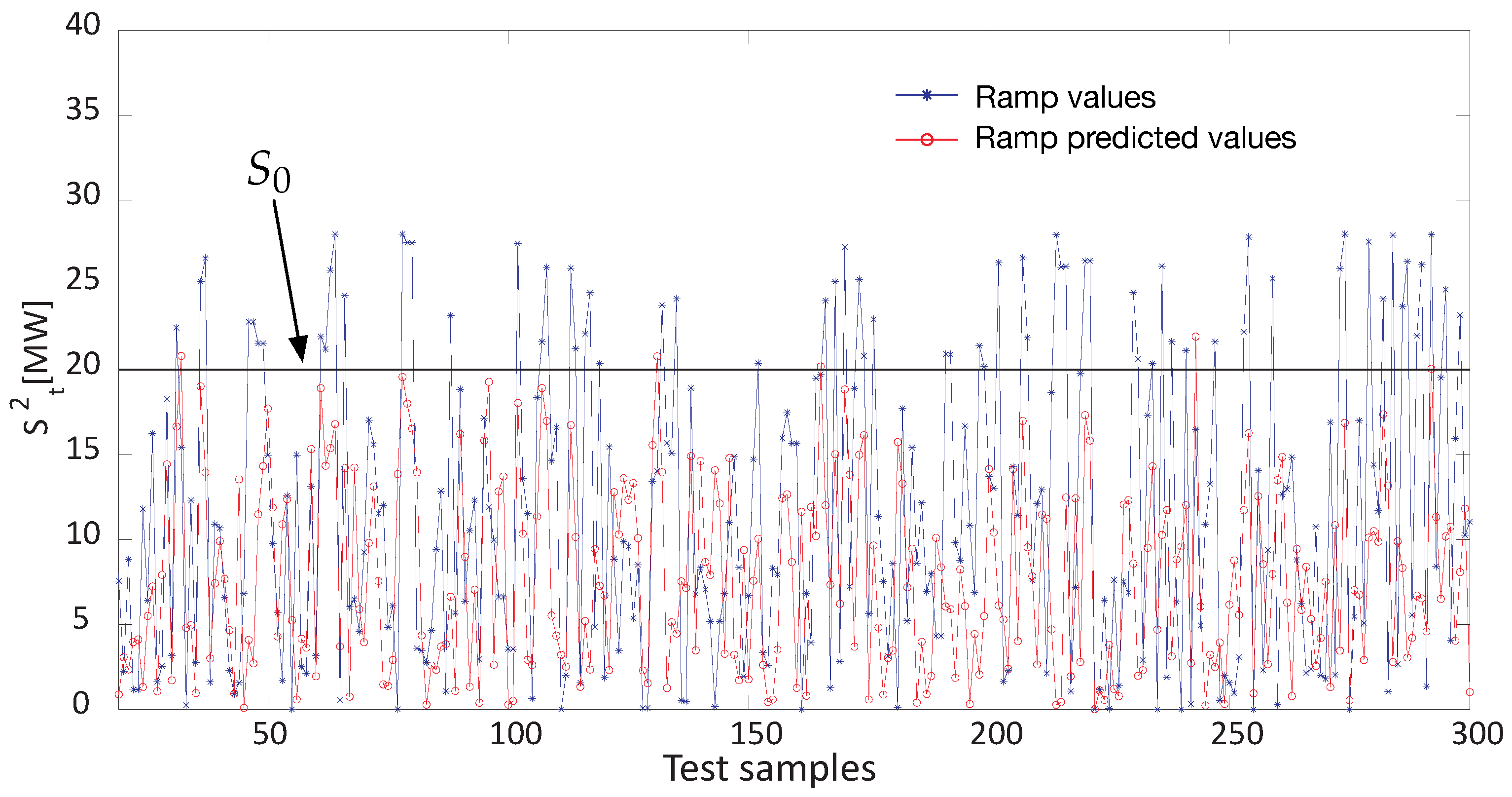
• Aiming at clearly showing the algorithms’ performance, only the 300 first samples of the test set have been represented in these figures.
• Furthermore, a threshold value $S_0$ (and the corresponding $-S_0$) has been marked in these figures, so it can be used to decide whether or not the event is a ramp power event (see Equation (3)). When a ramp occurs, it is possible to decide whether the ramp event is ascending or descending.

The results illustrated in Figure 2a show two data series: the series of real measured WPRE (red ∘) and the series of predicted WPRE (blue ∗) values computed by using the proposed hybrid methodology. In the effort to better explain the results and the applicability of our proposal, we have drawn Figure 2 in a more detailed way than the others, zooming into two shorter time excerpts, b and c. The insets b and c show how there are some WPREs that surpass any of the thresholds $S_0$ and $-S_0$. Specifically, and as mentioned before, a WPRE is detected in our approach if the ramp function is larger than 50% of $S_0$. Note that Figure 2b,c shows how the predicted WPREs (blue ∗) exceeding any thresholds ($S_0$ or $-S_0$) are correctly predicted when compared to the real, measured WPRE (red ∘).

Regarding such a threshold value, it is worth mentioning that $S_0$ is not used until the very end of the experiments, once the ramp function has been predicted with the ML regression algorithms. In this respect, it is also convenient to remark that, in the proposed approach, we do not look to optimize $S_0$. We only display $S_0$ as an indication (example) that the ML regression model $\mathcal{M}$ applied can be turned into a classification for WPRE. Note, however, that the purpose of our paper is to deal with it as a regression problem.

The good performance observed in Figure 2 for the EML is common (and even better) to those illustrated in Figure 3 and Figure 4.

The joint analysis of both Figure 2 and Figure 4 and Table 4 reveals the suitable throughput of the ML regression techniques (mainly the GPR model), which hybridized with the ERA-Interim predictive values, assist in obtaining a robust decision system in terms of the existence or not of a power ramp, depending, of course, on the definition of the threshold $S_0$.

6.1.2. Results Using $S_t^2$ as the Ramp Function Definition

On the other hand,

Table 5. Results (in terms of RMSE, MAE and sensitivity) corresponding to the estimation of the ramp function $S_t^2$ (Equation (2)) obtained by the proposed approach as a function of the ML regressors explored (SVR, ELM, GPR, and MLP), for Wind Farms “A”, “B” and “C”, respectively.

Wind Farm A
ML Regressor	RMSE (MW)	MAE (MW)	$\mathbf{s}$(ramp) %	$\mathbf{s}$(no ramp) %
SVR	6.8847	5.1876	31.33	96.27
ELM	5.7037	4.2925	41.99	95.01
GPR	5.2048	3.7897	49.66	96.36
MLP	5.4351	3.9861	8.71	99.44
Wind Farm B
ML Regressor	RMSE (MW)	MAE (MW)	$\mathbf{s}$(ramp) %	$\mathbf{s}$(no ramp) %
SVR	7.9439	5.8853	44.16	85.55
ELM	7.3148	5.8675	34.67	93.23
GPR	5.9223	4.4037	65.32	84.12
MLP	5.9051	4.3475	14.76	97.17
Wind Farm C
ML Regressor	RMSE (MW)	MAE (MW)	$\mathbf{s}$(ramp) %	$\mathbf{s}$(no ramp) %
SVR	7.1525	5.4677	37.88	93.83
ELM	5.8624	4.4368	58.16	92.10
GPR	5.1030	3.6991	57.26	94.42
MLP	5.0605	3.6670	11.22	98.56

and Figure 5, Figure 6 and Figure 7 will assist us in explaining the results when $S_t^2$ is the ramp function to be predicted.

Table 5 represents the results (in terms of RMSE, MAE and sensitivity) corresponding to the estimation of the ramp function $S_t^2$ (Expression (2)) achieved by using the proposed approach as a function of the ML regressors explored (SVR, ELM, GPR and MLP).

A first aspect that stands out in Table 5 is that it has fewer columns related to sensitivity than those of Table 4. This is an interesting points that arises from the different definitions of the ramp function $S_t^2$, either $S_t^1$ or $S_t^2$. Note that, for definition $S_t^2$, the sensitivity is the percentage of correctly predicted results (either ramp or no ramp) with respect to the actual measured data. This is the reason why s has only two columns in Table 5, s (ramp) and s (no ramp), whereas Table 4 exhibits three s-related columns. This is because, in the case of the $S_t^1$ ramp definition, there are three events to be detected: ascending ramp (+), descending ramp (−) and no ramps.

In the same way as Table 4, Table 5 also reveals that, for $S_t=S_t^2$, the GPR approach exhibits the best results, outperforming clearly the rest of the ML regressors tested, except the MLP. This has similar values only in its error metric, RMSE and MAE, but not in its s (ramp) value, which is considerably worse than that of the GPR. This is clear, for instance, in Wind Farm A, in which RMSE${}_{\mathrm{GPR}}\approx 5.20$ MW, less than that of the other regressors. Note that s(ramp)${}_{\mathrm{GPR}}=49.66\gg$s (ramp)${}_{\mathrm{MLP}}=8.71$. In Wind Farm B, the performance of the GPR (RMSE${}_{\mathrm{GPR}}\approx 5.90$ MW) is similar to that of the MLP and much better than that of SVR (RMSE${}_{\mathrm{SVR}}\approx 7.94$ MW) and SVR (RMSE${}_{\mathrm{SVR}}\approx 7.32$ MW). Note again that, although the GPR model is similar to the MLP in error metrics, however, the GPR exhibits much better sensitivity than the MLP, s (ramp)${}_{\mathrm{GPR}}\gg$s (ramp)${}_{\mathrm{MLP}}$. This is true not only for the MLP (which has similar errors), but also for the rest of the ML, which are long surpassed by the GPR model in the aim of detecting wind ramps. For clarity, we have marked this in bold in Table 5. This means that the GPR is more efficient in predicting wind ramps (the very core of our approach) than the others, and this is the reason why we say that the sensitivity helps supplement the information provided by the error metrics.

Once the results shown in Table 5 have already been analyzed, it is convenient to have a look at its associated figures showing the data series, which involve both the estimated (predicted) and the measured values of the ramp function $S_t^2$. Regarding this, Figure 5, Figure 6 and Figure 7 show the estimation of $S_t^2$ obtained by the GPR (in Wind Farm A) and ELM algorithms, for the wind farms B and C, respectively.

We have also represented in Figure 5, Figure 6 and Figure 7 a threshold value $S_0$ to mark the presence (or not) of a WPRE. As in the first objective function, the good performance of the ML regressors allows a significant detection of WPRE in wind farms.

6.2. Discussion

The results obtained show that the proposed hybrid WPREs prediction approach—which combines data from numerical-physical models (reanalysis) with state-of-the-art statistical ML approaches (regressors)—is a feasible option to tackle this problem in wind farms. Regarding the proposed fusion of reanalysis data and ML regressors, the results have pointed out that:

• The use of reanalysis data as predictive variables for WPRE forecast has the following beneficial properties:
  • Reanalysis makes the training of the ML regressors easier if there are enough measures of the objective variables. This is just the case in our approach because reanalysis data provide robust meteorological variable estimation back to 1979 in the case of the ERA-Interim reanalysis, with high spatial and enough temporal resolution to tackle this problem.
  • The variables from reanalysis projects are similar to those by any weather numerical forecast system, even meso-scale ones, so it is straightforward to tackle the WPRE prediction by using alternative models, such as the well-known Weather Research and Forecasting (WRF) meso-scale model [91], to predict future values of the predictive variables and, then, the corresponding WPRE prediction for a given wind farm.
  • The use of reanalysis data allows the repeatability of the described experiments by other researchers since such data are freely available on the Internet.
• The performance studies of the state-of-the-art ML regressors, the other pillar our approach is based on, have shown that the GPR reaches the best results in both definitions of the wind power ramp function considered:
  • When using the $S_t^1$ definition, the results clearly show that the GPR model achieves the best results of all the regressors tested, with an accurate reconstruction of the ramp function from the ERA-Interim variables. Its RMSE and MAE vales are much lower than those of the other ML regressors explored. Furthermore, its sensitivity s—or percentage of correct predictions (with respect to the real, measured data)—is much higher than those provided by the other regressors: s (+ramp)${}_{\mathrm{GPR}}\gg$s (+ramp)${}_{\mathrm{others}}$ (for ascending ramps) and s (−ramp)${}_{\mathrm{GPR}}\gg$s(−ramp)${}_{\mathrm{others}}$ (for descending ramps). This demonstrates the feasibility of the proposed methodology for predicting wind ramps, both ascending and descending ones.
  • Similarly, when using the $S_t^2$ ramp definition, the GPR approach also exhibits the best results, outperforming clearly the rest of the ML regressors tested, except the MLP, which has similar values only in its error metric, RMSE and MAE, but not in its s(ramp) value, which is considerably worse than that of the GPR. These sensitivity results point out that the GPR is more efficient in predicting wind ramps (the very core of our approach) than the other regressors, this being the reason why we have mentioned that the sensitivity metric helps complement the information provided by the error measures.

Finally, the results show how the proposed approach allows the use of threshold values to detect whether or not a wind power ramp occurs. The method is also flexible enough to choose a ramp function definition in the aim of considering a multi-class problem. Although in the experiments carried out, the multi-class problem contains three classes (ascending, descending or not ramp, in the $S_t^1$ definition), more classes could be defined. The optimal selection of the threshold values is an open question in the literature that has not been considered in this case.

7. Conclusions

In this paper, we have explored the feasibility of a novel hybrid approach that—by combining data from numerical-physical models (reanalysis) and state-of-the-art statistical Machine Learning (ML) regressors—aims at predicting Wind Power Ramp Events (WPREs). The accurate prediction of WPREs—caused by large fluctuations of wind power in a short time interval lead—is of practical interest not only for utility companies and independent system operators (in the effort of efficiently integrating wind energy without affecting power grid stability), but also for wind power farm owners (to reduce damage in turbines).

Specifically, several state-of-the-art statistical ML regressors—ranging from a Multi-Layer Perceptron (MLP) neural network to an Extreme Learning Machine (ELM), a Gaussian Process Regression (GPR) or a Support Vector Regression (SVR) algorithm—have been applied to solve this problem in three different wind farms in Spain.

This has been the first contribution of our proposal since the use of regressors has not been previously applied directly to this WPRE prediction problem. The second contribution has been the use of direct reanalysis data as input (predictive) variables of the ML regression techniques. In this regard, we have proposed the use of data from the ERA-Interim reanalysis because it ensures a high resolution of the inputs, both spatial (grid of 0.125 × 0.125 at global level) and temporal (6-h time horizon). Two other reasons why we have used reanalysis are: (a) the use of reanalysis data allows the repeatability of the experiments by other researchers since such data are available on the Internet; (b) the variables from reanalysis are similar to those from weather numerical forecast systems, even mesoscale ones, so that it would be straightforward to tackle the WPRE prediction problem by using other alternative models. Note however that it would be possible to adapt the proposed regression techniques to operate with alternative data not coming from numerical methods (or reanalysis), but other types of input variables.

Our purpose has been modeling the wind ramp function as accurately as possible in terms of several input variables. This way of tackling the problem overcomes some problems associated with the WPRE defined as a binary classification task [43,44], or even ordinal classification [73], such as the appearance of highly imbalanced problems.

We have considered two different definitions of the ramp function, those that are used the most in the literature. The experimental work has been carried out using data corresponding to three wind farms, located in different zones of Spain and having different atmospheric conditions, in the effort to obtain results as generalizable as possible. The experimental work carried out basically points out that:

• The results show a good performance of the explored ML regression techniques hybridized with the ERA-Interim reanalysis data, especially those corresponding to the ELM and the GPR ML regressors. In particular, the GPR has been found to exhibit the best results, outperforming clearly the rest of the ML regressors tested. This has been shown especially evident in terms of its sensitivity (or percentage of correct predictions (with respect to the real, measured data)), which is much higher than those provided by the other regressors, showing the feasibility of the proposed methodology for predicting WPREs.
• The experimental work has also revealed that the use of reanalysis data as predictive variables for WPRE forecast is beneficial: reanalysis has been found to make the training of the ML regressors easier since the ERA-Interim reanalysis provides robust meteorological variable estimation back to 1979, with high spatial and enough temporal resolution to tackle this problem.

As a general conclusion, the results achieved by the proposed approach show that our hybrid method is a feasible alternative to deal with the important problems that WPREs can cause in both the management of wind farms and in the balanced operation of power grids.

References

1. Kumar, Y.; Ringenberg, J.; Depuru, S.S.; Devabhaktuni, V.K.; Lee, J.W.; Nikolaidis, E.; Andersen, B.; Afjeh, A. Wind energy: Trends and enabling technologies. Renew. Sustain. Energy Rev. 2016, 53, 209–224. [Google Scholar] [CrossRef]
2. Brenna, M.; Foiadelli, F.; Longo, M.; Zaninelli, D. Improvement of Wind Energy Production through HVDC Systems. Energies 2017, 10, 157. [Google Scholar] [CrossRef]
3. Mohagheghi, E.; Gabash, A.; Li, P. A Framework for Real-Time Optimal Power Flow under Wind Energy Penetration. Energies 2017, 10, 535. [Google Scholar] [CrossRef]
4. Ali, S.; Lee, S.M.; Jang, C.M. Techno-Economic Assessment of Wind Energy Potential at Three Locations in South Korea Using Long-Term Measured Wind Data. Energies 2017, 10, 1442. [Google Scholar] [CrossRef]
5. Dai, H.; Herran, D.S.; Fujimori, S.; Masui, T. Key factors affecting long-term penetration of global onshore wind energy integrating top-down and bottom-up approaches. Renew. Energy 2016, 85, 19–30. [Google Scholar] [CrossRef]
6. Colmenar-Santos, A.; Perera-Perez, J.; Borge-Diez, D. Offshore wind energy: A review of the current status, challenges and future development in Spain. Renew. Sustain. Energy Rev. 2016, 64, 1–18. [Google Scholar] [CrossRef]
7. Giebel, G.; Hasager, C.B. An Overview of Offshore Wind Farm Design. In MARE-WINT; Springer: Cham, Switzerland, 2016; pp. 337–346. [Google Scholar]
8. Herbert, G.J.; Iniyan, S.; Amutha, D. A review of technical issues on the development of wind farms. Renew. Sustain. Energy Rev. 2014, 32, 619–641. [Google Scholar] [CrossRef]
9. Lunney, E.; Ban, M.; Duic, N.; Foley, A. A state-of-the-art review and feasibility analysis of high altitude wind power in Northern Ireland. Renew. Sustain. Energy Rev. 2017, 68, 899–911. [Google Scholar] [CrossRef]
10. Jangid, J.; Bera, A.K.; Joseph, M.; Singh, V.; Singh, T.; Pradhan, B.; Das, S. Potential zones identification for harvesting wind energy resources in desert region of India—A multi criteria evaluation approach using remote sensing and GIS. Renew. Sustain. Energy Rev. 2016, 65, 1–10. [Google Scholar] [CrossRef]
11. Simões, T.; Estanqueiro, A. A new methodology for urban wind resource assessment. Renew. Energy 2016, 89, 598–605. [Google Scholar] [CrossRef]
12. Köktürk, G.; Tokuç, A. Vision for wind energy with a smart grid in Izmir. Renew. Sustain. Energy Rev. 2017, 73, 332–345. [Google Scholar] [CrossRef]
13. Peters, G.P.; Andrew, R.M.; Boden, T.; Canadell, J.G.; Ciais, P.; Le Quéré, C.; Marland, G.; Raupach, M.R.; Wilson, C. The challenge to keep global warming below 2 °C. Nat. Clim. Chang. 2013, 3, 4–6. [Google Scholar] [CrossRef]
14. Bauer, N.; Bosetti, V.; Hamdi-Cherif, M.; Kitous, A.; McCollum, D.; Méjean, A.; Rao, S.; Turton, H.; Paroussos, L.; Ashina, S.; et al. CO2 emission mitigation and fossil fuel markets: Dynamic and international aspects of climate policies. Technol. Forecast. Soc. Chang. 2015, 90, 243–256. [Google Scholar] [CrossRef] [Green Version]
15. Jones, L.E. Renew. Energy Integration: Practical Management of Variability, Uncertainty, and Flexibility in Power Grids; Academic Press: Cambridge, MA, USA, 2017. [Google Scholar]
16. Cuadra, L.; Pino, M.D.; Nieto-Borge, J.C.; Salcedo-Sanz, S. Optimizing the Structure of Distribution Smart Grids with Renewable Generation against Abnormal Conditions: A Complex Networks Approach with Evolutionary Algorithms. Energies 2017, 10, 1097. [Google Scholar] [CrossRef]
17. Cuadra, L.; Salcedo-Sanz, S.; Del Ser, J.; Jiménez-Fernández, S.; Geem, Z.W. A critical review of robustness in power grids using complex networks concepts. Energies 2015, 8, 9211–9265. [Google Scholar] [CrossRef] [Green Version]
18. Yan, J.; Liu, Y.; Han, S.; Wang, Y.; Feng, S. Reviews on uncertainty analysis of wind power forecasting. Renew. Sustain. Energy Rev. 2015, 52, 1322–1330. [Google Scholar] [CrossRef]
19. Cabrera-Tobar, A.; Bullich-Massagué, E.; Aragüés-Peñalba, M.; Gomis-Bellmunt, O. Review of advanced grid requirements for the integration of large scale photovoltaic power plants in the transmission system. Renew. Sustain. Energy Rev. 2016, 62, 971–987. [Google Scholar] [CrossRef]
20. Cuadra, L.; Salcedo-Sanz, S.; Nieto-Borge, J.; Alexandre, E.; Rodríguez, G. Computational intelligence in wave energy: Comprehensive review and case study. Renew. Sustain. Energy Rev. 2016, 58, 1223–1246. [Google Scholar] [CrossRef]
21. Kroposki, B.; Johnson, B.; Zhang, Y.; Gevorgian, V.; Denholm, P.; Hodge, B.M.; Hannegan, B. Achieving a 100% renewable grid: Operating electric power systems with extremely high levels of variable renewable energy. IEEE Power Energy Mag. 2017, 15, 61–73. [Google Scholar] [CrossRef]
22. Yoldaş, Y.; Önen, A.; Muyeen, S.; Vasilakos, A.V.; Alan, İ. Enhancing smart grid with microgrids: Challenges and opportunities. Renew. Sustain. Energy Rev. 2017, 72, 205–214. [Google Scholar] [CrossRef]
23. Gough, R.; Dickerson, C.; Rowley, P.; Walsh, C. Vehicle-to-grid feasibility: A techno-economic analysis of EV-based energy storage. Appl. Energy 2017, 192, 12–23. [Google Scholar] [CrossRef]
24. Zhao, Y.; Noori, M.; Tatari, O. Boosting the adoption and the reliability of renewable energy sources: Mitigating the large-scale wind power intermittency through vehicle to grid technology. Energy 2017, 120, 608–618. [Google Scholar] [CrossRef]
25. Renani, E.T.; Elias, M.F.M.; Rahim, N.A. Using data-driven approach for wind power prediction: A comparative study. Energy Convers. Manag. 2016, 118, 193–203. [Google Scholar] [CrossRef]
26. Tascikaraoglu, A.; Uzunoglu, M. A review of combined approaches for prediction of short-term wind speed and power. Renew. Sustain. Energy Rev. 2014, 34, 243–254. [Google Scholar] [CrossRef]
27. Zhang, J.; Cui, M.; Hodge, B.M.; Florita, A.; Freedman, J. Ramp forecasting performance from improved short-term wind power forecasting over multiple spatial and temporal scales. Energy 2017, 122, 528–541. [Google Scholar] [CrossRef]
28. Gallego-Castillo, C.; Cuerva-Tejero, A.; Lopez-Garcia, O. A review on the recent history of wind power ramp forecasting. Renew. Sustain. Energy Rev. 2015, 52, 1148–1157. [Google Scholar] [CrossRef]
29. Ouyang, T.; Zha, X.; Qin, L. A survey of wind power ramp forecasting. Energy Power Eng. 2013, 5, 368–372. [Google Scholar] [CrossRef]
30. Alizadeh, M.; Moghaddam, M.P.; Amjady, N.; Siano, P.; Sheikh-El-Eslami, M. Flexibility in future power systems with high renewable penetration: A review. Renew. Sustain. Energy Rev. 2016, 57, 1186–1193. [Google Scholar] [CrossRef]
31. Ferreira, C.; Gama, J.; Matias, L.; Botterud, A.; Wang, J. A survey on Wind Power Ramp Forecasting; Technical Report; Argonne National Laboratory (ANL): Lemont, IL, USA, 2011. [Google Scholar]
32. Gallego-Castillo, C.; Garcia-Bustamante, E.; Cuerva, A.; Navarro, J. Identifying wind power ramp causes from multivariate datasets: A methodological proposal and its application to reanalysis data. IET Renew. Power Gener. 2015, 9, 867–875. [Google Scholar] [CrossRef]
33. Ohba, M.; Kadokura, S.; Nohara, D. Impacts of synoptic circulation patterns on wind power ramp events in East Japan. Renew. Energy 2016, 96, 591–602. [Google Scholar] [CrossRef]
34. Salcedo-Sanz, S.; Pérez-Bellido, A.M.; Ortiz-García, E.G.; Portilla-Figueras, A.; Prieto, L.; Paredes, D. Hybridizing the fifth generation mesoscale model with artificial neural networks for short-term wind speed prediction. Renew. Energy 2009, 34, 1451–1457. [Google Scholar] [CrossRef]
35. Drew, D.R.; Cannon, D.J.; Barlow, J.F.; Coker, P.J.; Frame, T.H. The importance of forecasting regional wind power ramping: A case study for the UK. Renew. Energy 2017, 114, 1201–1208. [Google Scholar] [CrossRef]
36. Cui, M.; Ke, D.; Sun, Y.; Gan, D.; Zhang, J.; Hodge, B.M. Wind power ramp event forecasting using a stochastic scenario generation method. IEEE Trans. Sustain. Energy 2015, 6, 422–433. [Google Scholar]
37. Foley, A.M.; Leahy, P.G.; Marvuglia, A.; McKeogh, E.J. Current methods and advances in forecasting of wind power generation. Renew. Energy 2012, 37, 1–8. [Google Scholar] [CrossRef] [Green Version]
38. Salcedo-Sanz, S. Modern meta-heuristics based on nonlinear physics processes: A review of models and design procedures. Phys. Rep. 2016, 655, 1–70. [Google Scholar] [CrossRef]
39. De Jong, K.A. Evolutionary Computation: A Unified Approach; MIT Press: Cambridge, MA, USA, 2006. [Google Scholar]
40. Ata, R. Artificial neural networks applications in wind energy systems: A review. Renew. Sustain. Energy Rev. 2015, 49, 534–562. [Google Scholar] [CrossRef]
41. Suganthi, L.; Iniyan, S.; Samuel, A.A. Applications of fuzzy logic in renewable energy systems—A review. Renew. Sustain. Energy Rev. 2015, 48, 585–607. [Google Scholar] [CrossRef]
42. Salcedo-Sanz, S.; Pastor-Sánchez, A.; Del Ser, J.; Prieto, L.; Geem, Z.W. A Coral Reefs Optimization algorithm with Harmony Search operators for accurate wind speed prediction. Renew. Energy 2015, 75, 93–101. [Google Scholar] [CrossRef]
43. Dorado-Moreno, M.; Cornejo-Bueno, L.; Gutiérrez, P.; Prieto, L.; Hervás-Martínez, C.; Salcedo-Sanz, S. Robust estimation of wind power ramp events with reservoir computing. Renew. Energy 2017, 111, 428–437. [Google Scholar] [CrossRef]
44. Cornejo-Bueno, L.; Aybar-Ruiz, A.; Camacho-Gómez, C.; Prieto, L.; Barea-Ropero, A.; Salcedo-Sanz, S. A Hybrid Neuro-Evolutionary Algorithm for Wind Power Ramp Events Detection. In Proceedings of the International Work-Conference on Artificial Neural Networks, Cadiz, Spain, 14–16 June 2017; Springer: Cham, Switzerland, 2017; pp. 745–756. [Google Scholar]
45. Botterud, A.; Wang, J.; Miranda, V.; Bessa, R.J. Wind power forecasting in US electricity markets. Electr. J. 2010, 23, 71–82. [Google Scholar] [CrossRef]
46. Fang, S.; Chiang, H.D. Improving supervised wind power forecasting models using extended numerical weather variables and unlabelled data. IET Renew. Power Gener. 2016, 10, 1616–1624. [Google Scholar] [CrossRef]
47. Costa, A.; Crespo, A.; Navarro, J.; Lizcano, G.; Madsen, H.; Feitosa, E. A review on the young history of the wind power short-term prediction. Renew. Sustain. Energy Rev. 2008, 12, 1725–1744. [Google Scholar] [CrossRef] [Green Version]
48. Al-Yahyai, S.; Charabi, Y.; Gastli, A. Review of the use of Numerical Weather Prediction (NWP) Models for wind energy assessment. Renew. Sustain. Energy Rev. 2010, 14, 3192–3198. [Google Scholar] [CrossRef]
49. Cutler, N.; Kay, M.; Jacka, K.; Nielsen, T.S. Detecting, categorizing and forecasting large ramps in wind farm power output using meteorological observations and WPPT. Wind Energy 2007, 10, 453–470. [Google Scholar] [CrossRef]
50. Bossavy, A.; Girard, R.; Kariniotakis, G. Forecasting ramps of wind power production with numerical weather prediction ensembles. Wind Energy 2013, 16, 51–63. [Google Scholar] [CrossRef]
51. Haupt, S.E.; Wiener, G.; Liu, Y.; Myers, B.; Sun, J.; Johnson, D.; Mahoney, W. A wind power forecasting system to optimize power integration. In Proceedings of the ASME 2011 5th International Conference on Energy Sustainability, Washington, DC, USA, 7–10 August 2011; American Society of Mechanical Engineers: New York, NY, USA, 2011; pp. 2215–2222. [Google Scholar]
52. Martínez-Arellano, G. Forecasting Wind Power for the Day-Ahead Market Using Numerical Weather Prediction Models and Computational Intelligence Techniques. Ph.D. Thesis, Nottingham Trent University, Nottingham, UK, 2015. [Google Scholar]
53. Dabernig, M. Comparison of Different Numerical Weather Prediction Models as Input for Statistical Wind Power Forecasts. Ph.D. Thesis, University of Innsbruck, Innsbruck, Austria, 2013. [Google Scholar]
54. Bianco, L.; Djalalova, I.V.; Wilczak, J.M.; Cline, J.; Calvert, S.; Konopleva-Akish, E.; Finley, C.; Freedman, J. A wind energy ramp tool and metric for measuring the skill of numerical weather prediction models. Weather Forecast. 2016, 31, 1137–1156. [Google Scholar] [CrossRef]
55. Cutler, N.J.; Outhred, H.R.; MacGill, I.F.; Kay, M.J.; Kepert, J.D. Characterizing future large, rapid changes in aggregated wind power using numerical weather prediction spatial fields. Wind Energy 2009, 12, 542–555. [Google Scholar] [CrossRef]
56. Greaves, B.; Collins, J.; Parkes, J.; Tindal, A. Temporal forecast uncertainty for ramp events. Wind Eng. 2009, 33, 309–319. [Google Scholar] [CrossRef]
57. Carvalho, D.; Rocha, A.; Gómez-Gesteira, M.; Santos, C.S. Offshore winds and wind energy production estimates derived from ASCAT, OSCAT, numerical weather prediction models and buoys—A comparative study for the Iberian Peninsula Atlantic coast. Renew. Energy 2017, 102, 433–444. [Google Scholar] [CrossRef]
58. Andrade, J.R.; Bessa, R.J. Improving renewable energy forecasting with a grid of numerical weather predictions. IEEE Trans. Sustain. Energy 2017, 8, 1571–1580. [Google Scholar] [CrossRef]
59. Cannon, D.; Brayshaw, D.; Methven, J.; Drew, D. Determining the bounds of skilful forecast range for probabilistic prediction of system-wide wind power generation. Meteorol. Z. 2016, 26, 239–252. [Google Scholar] [CrossRef]
60. Milanese, M.; Tornese, L.; Colangelo, G.; Laforgia, D.; de Risi, A. Numerical method for wind energy analysis applied to Apulia Region, Italy. Energy 2017, 128, 1–10. [Google Scholar] [CrossRef]
61. Kung, S.Y. Kernel Methods and Machine Learning; Cambridge University Press: Cambridge, UK, 2014. [Google Scholar]
62. Berk, R.A. Support Vector Machines. In Statistical Learning from a Regression Perspective; Springer International Publishing: Cham, Switzerland, 2016; pp. 291–310. [Google Scholar]
63. Huang, G.; Huang, G.B.; Song, S.; You, K. Trends in extreme learning machines: A review. Neural Netw. 2015, 61, 32–48. [Google Scholar] [CrossRef] [PubMed]
64. Soman, S.S.; Zareipour, H.; Malik, O.; Mandal, P. A review of wind power and wind speed forecasting methods with different time horizons. In Proceedings of the 2010 North American Power Symposium (NAPS), Arlington, TX, USA, 26–28 September 2010; pp. 1–8. [Google Scholar]
65. Barber, C.; Bockhorst, J.; Roebber, P. Auto-regressive HMM inference with incomplete data for short-horizon wind forecasting. In Advances in Neural Information Processing Systems; Neural Information Processing Systems Foundation, Inc.: Barcelona, Spain, 2010; pp. 136–144. [Google Scholar]
66. Zheng, H.; Kusiak, A. Prediction of wind farm power ramp rates: A data-mining approach. J. Sol. Energy Eng. 2009, 131, 031011. [Google Scholar] [CrossRef]
67. Hatano, K. A simpler analysis of the multi-way branching decision tree boosting algorithm. In Proceedings of the International Conference on Algorithmic Learning Theory, Sydney, Australia, 11–13 December 2001; Springer: Berlin/ Heidelberg, Germany, 2001; pp. 77–91. [Google Scholar]
68. Sevlian, R.; Rajagopal, R. Detection and statistics of wind power ramps. IEEE Trans. Power Syst. 2013, 28, 3610–3620. [Google Scholar] [CrossRef]
69. Gallego, C.; Costa, A.; Cuerva, A. Improving short-term forecasting during ramp events by means of regime-switching artificial neural networks. Adv. Sci. Res. 2011, 6, 55–58. [Google Scholar] [CrossRef]
70. Zareipour, H.; Huang, D.; Rosehart, W. Wind power ramp events classification and forecasting: A data mining approach. In Proceedings of the 2011 IEEE Power and Energy Society General Meeting, Detroit, MI, USA, 24–29 July 2011; pp. 1–3. [Google Scholar]
71. Cui, M.; Zhang, J.; Florita, A.R.; Hodge, B.M.; Ke, D.; Sun, Y. An optimized swinging door algorithm for wind power ramp event detection. In Proceedings of the 2015 IEEE Power & Energy Society General Meeting, Denver, CO, USA, 26–30 July 2015; pp. 1–5. [Google Scholar]
72. Bossavy, A.; Girard, R.; Kariniotakis, G. An edge model for the evaluation of wind power ramps characterization approaches. Wind Energy 2015, 18, 1169–1184. [Google Scholar] [CrossRef]
73. Dorado-Moreno, M.; Cornejo-Bueno, L.; Gutiérrez, P.A.; Prieto, L.; Salcedo-Sanz, S.; Hervás-Martínez, C. Combining Reservoir Computing and Over-Sampling for Ordinal Wind Power Ramp Prediction. In Proceedings of the International Work-Conference on Artificial Neural Networks, Cadiz, Spain, 14–16 June 2017; Springer: Cham, Switzerland, 2017; pp. 708–719. [Google Scholar]
74. Dorado-Moreno, M.; Durán-Rosal, A.M.; Guijo-Rubio, D.; Gutiérrez, P.A.; Prieto, L.; Salcedo-Sanz, S.; Hervás-Martínez, C. Multiclass prediction of wind power ramp events combining reservoir computing and support vector machines. In Proceedings of the Conference of the Spanish Association for Artificial Intelligence, Salamanca, Spain, 14–16 September 2016; Springer: Cham, Switzerland, 2016; pp. 300–309. [Google Scholar]
75. Dee, D.P.; Uppala, S.; Simmons, A.; Berrisford, P.; Poli, P.; Kobayashi, S.; Andrae, U.; Balmaseda, M.; Balsamo, G.; Bauer, P.; et al. The ERA-Interim reanalysis: Configuration and performance of the data assimilation system. Q. J. R. Meteorol. Soc. 2011, 137, 553–597. [Google Scholar] [CrossRef]
76. Smola, A.J.; Schölkopf, B. A tutorial on support vector regression. Stat. Comput. 2004, 14, 199–222. [Google Scholar] [CrossRef]
77. Salcedo-Sanz, S.; Rojo-Álvarez, J.L.; Martínez-Ramón, M.; Camps-Valls, G. Support vector machines in engineering: An overview. Wiley Interdiscip. Rev. Data Min. Knowl. Discov. 2014, 4, 234–267. [Google Scholar] [CrossRef]
78. Chang, C.C.; Lin, C.J. LIBSVM: A Library for Support Vector Machines. ACM Trans. Intell. Syst. Technol. 2011, 2. [Google Scholar] [CrossRef]
79. Chang, C.C.; Lin, C.J. LIBSVM: A Library for Support Vector Machines. Available online: https://www.csie.ntu.edu.tw/~cjlin/libsvm/ (accessed on 21 September 2017).
80. Haykin, S. Neural Networks: A Comprehensive Foundation; Prentice Hall PTR: Upper Saddle River, NJ, USA, 1994. [Google Scholar]
81. Bishop, C.M. Neural Networks for Pattern Recognition; Oxford University Press: Oxford, UK, 1995. [Google Scholar]
82. Hagan, M.T.; Menhaj, M.B. Training feedforward networks with the Marquardt algorithm. IEEE Trans. Neural Netw. 1994, 5, 989–993. [Google Scholar] [CrossRef] [PubMed]
83. Huang, G.B.; Zhu, Q.Y.; Siew, C.K. Extreme learning machine: Theory and applications. Neurocomputing 2006, 70, 489–501. [Google Scholar] [CrossRef]
84. Huang, G.B.; Zhou, H.; Ding, X.; Zhang, R. Extreme learning machine for regression and multiclass classification. IEEE Trans. Syst. Man Cybern. Part B 2012, 42, 513–529. [Google Scholar] [CrossRef] [PubMed]
85. Huang, G.B. ELM Matlab Code. Available online: http://www.ntu.edu.sg/home/egbhuang/elm_codes.html (accessed on 20 August 2017).
86. Rasmussen, C.E.; Williams, C.K. Gaussian Processes for Machine Learning; MIT Press: Cambridge, MA, USA, 2006; Volume 1. [Google Scholar]
87. Lázaro-Gredilla, M.; Van Vaerenbergh, S.; Lawrence, N.D. Overlapping mixtures of Gaussian processes for the data association problem. Pattern Recognit. 2012, 45, 1386–1395. [Google Scholar] [CrossRef]
88. Hu, J.; Wang, J. Short-term wind speed prediction using empirical wavelet transform and Gaussian process regression. Energy 2015, 93, 1456–1466. [Google Scholar] [CrossRef]
89. Camps-Valls, G. Simple Regression Toolbox (SimpleR). Available online: http://www.uv.es/gcamps/software.html (accessed on 1 August 2017).
90. Gallego Castillo, C.J. Statistical Models for Short-Term Wind Power Ramp Forecasting. Ph.D. Thesis, Polytechnic School of Aeronautical Engineers, Universidad Politécnica de Madrid, Madrid, Spain, 2013. [Google Scholar]
91. Skamarock, W.C.; Klemp, J.B.; Dudhia, J.; Gill, D.O.; Barker, D.M.; Wang, W.; Powers, J.G. A Description of the Advanced Research WRF Version 2; Technical Report; Mesoscale and Microscale Meteorology Division, National Center for Atmospheric Research: Boulder, CO, USA, 2005. [Google Scholar]
Figure 1. Representation of the geographical location of the wind farms (labeled “A”, “B” and “C”) considered in the experimental work carried out in this paper. The four closest nodes from the Era-Interim reanalysis (predictive variables) have also been represented for illustrative purposes. The reason why these wind farms have been selected is that they cover different parts of Spain, north, center and south, characterized by different wind regimes.
Energies 10 01784 g001
Figure 2. (a) Estimation of the ramp function S t 1 (Equation (1)) obtained by using the proposed approach in the particular case in which the ML is an ELM regressor. This figure corresponds to Wind Farm A, whose location has been represented in Figure 1. (b,c) represent two shorter excerpts in which the predicted WPREs that exceed the thresholds ( S 0 or S 0 ) are shown to be correctly detected. A WPRE is detected if S t 1 > 0.5 S 0 . The predicted series exhibits RMSE 5.68 MW, MAE 4.25 MW, s (+ramp) = 40.54 % , s (−ramp) = 42.59 % and s (no ramp) = 95.51 % .
Energies 10 01784 g002
Figure 3. Estimation of the ramp function S t 1 (Equation (1)) obtained by our proposed hybrid approach when using the GPR as the ML regressor in Wind Farm B. The predicted series exhibits RMSE 5.98 MW, MAE 4.43 MW, s (+ramp) = 52.10 % , s (−ramp) = 58.25 % and s (no ramp) = 91.71 % (see Table 4).
Energies 10 01784 g003
Figure 4. Prediction of the ramp function S t 1 (Equation (1)) when using the GPR in Wind Farm C. The predicted ramps series exhibits RMSE 4.75 MW, MAE 3.48 MW, s (+ramp) = 57.14 % , s (−ramp) = 61.05 % , and s (no ramp) = 93.99 % (see Table 4).
Energies 10 01784 g004
Figure 5. Estimation of the ramp function S t 2 (Equation (2)) obtained by the proposed approach using the GPR regressor, in Wind Farm A. The ramp predicted values resemble the ramp measured ones with RMSE 5.20 MW and MAE 3.79 MW, s (ramp) = 49.66 % and s (no ramp) = 96.36 % (see Table 5).
Energies 10 01784 g005
Figure 6. Estimation of the ramp function S t 2 (Expression (2)) obtained by the proposed method when using the ELM regressor, in Wind Farm B. The predicted series follows the measured series with RMSE 5.90 MW and MAE 4.40 MW, s (ramp) = 65.32 % and s (no ramp) = 84.12 % (see Table 5).
Energies 10 01784 g006
Figure 7. Estimation of the ramp function S t 2 (Expression (2)) obtained by the proposed method when using the ELM regressor, in Wind Farm C. The predicted series follows the measured series with RMSE 5.86 MW and MAE 4.43 MW, s (ramp) = 58.16 % and s (no ramp) = 92.10 % (see Table 5).
Energies 10 01784 g007