Evaluation Method for the Firm Power Escalation of a Wind-Storage Hybrid Power System

Abstract

To improve the controllability of the electric power output and the economic performance of a large-scale wind farm, an auxiliary energy storage system is required. This paper deals with the rule of planning reasonable energy storage power and capacity based on the historical annual mean wind speed data, the probability density of the pulsating wind power output, and the warranted firm power provided by the wind farm. Specifically, the evaluation index of the fluctuation degree of the firm power is defined in order to optimize the planned energy storage capacity. After that, the firm power escalation affected by the energy storage power and the conversion rate of the storage device are quantitatively evaluated. All of these analyses contribute in a significant way towards determining the acceptable energy conversion rate with the condition of limited energy storage space of a wind-storage hybrid power system. The proposed evaluation method of the firm power escalation is verified by MatLab simulation results.

1. Introduction

Installed wind energy capacity is growing rapidly throughout the world because it is readily available, environmentally friendly, and cost effective in all manners [1,2]. However, the negative impact on the power grid also becomes increasingly apparent when it comes to large-scale wind farms due to the intermittent nature and volatility of wind speed [3]. The random variation of the wind power output leads to a lower rotational inertia level of generators and a worse frequency regulation characteristic [4]. On the other hand, the probability of power grid voltage fluctuation and voltage flicker, which may lead to cascading trip-off of wind turbine generators, is increased [5]. One way to solve these problems is to utilize the complementary energy sources distributed in different regions; another way is to allocate the spinning reserve. For China, the power network structures are less robust than those in European countries while the installed capacity of a single wind farm may be as large as 200 MW. As a result, the wind-storage hybrid power system has been developing and now presents a choice by which the requirements of power balance and power stability of the grid can be met. In spite of the fact that the wind power systems in China focus on generating whatever amount of wind energy is available [6], planning for a grid-connected scale of wind power is still limited by the dispatching department. Therefore, the economic interests of the wind farm are sacrificed due to wind curtailment. A rule for planning reasonable energy storage power and capacity is discussed in this paper as a way to improve the economic performance of a large-scale wind farm; these factors affect not only the reserve cost, but also the wind farm power output by regulating performance.

Studies of the rule for computing the energy storage power and capacity of a wind-storage hybrid power system have been carried out in different ways [7,8,9,10,11,12]. In Ref. [9], a method was proposed to compute the required energy storage capacity for long-term stable power output of a large-scale wind farm based on the characteristic function of a wind power generation unit’s output power and the probability distribution function of wind speed in the wind farm. The regulation goal of this method would enable the power output of the wind farm to maintain an average level. From this perspective, the calculated energy storage capacity may be much higher than necessary because the power output of wind turbines under maximum power point tracking mode varies with the wind speed and it is not practical to be horizontal line modeled. Thus, in this paper, the regulation goal of the wind farm output tracks the stable power component of the wind turbines’ power output, which represents the highest level of the acceptance ability of the grid for wind power. In Ref. [10], a battery energy storage system was designed using a buffer scheme to attenuate the effects of unsteady input power from wind farms, and the capacity of the system was determined by maximizing an objective function that measures the economic benefit obtainable from the dispatched power against the cost. However, the sample size of the daily data of the illustrative examples is too small to make such a determination. Thus, in this paper, the computing rule is based on the historical annual mean wind speed data, the probability density of the pulsating wind power output, and the warranted firm power provided by the wind farm. In Ref. [11], a quantitative criterion was proposed to identify the level of smoothing (LOS) of the power curve and a short-term neural network model was established to reflect the relationship between the characteristic parameters of the hybrid energy storage system (HESS), the LOS of output power transmitted to the grid, and the economic cost of the HESS. The genetic algorithm was then used to determine the optimal characteristic parameters of the HESS by optimizing the objective function. However, the energy storage space of the equipment on both sides—of the wind farm and the power grid—should not be equal. Thus, in this paper, the excessive wind power and the power shortage of the wind farm are contrastively analyzed when discussing the reasonable energy storage space. The authors of Refs. [9,10,11] were focused on the control principles and storage capacity of the energy storage system, but they did not consider how the wind power output was affected by the conversion rate of the energy storage equipment, and none of them proposed any evaluation index or evaluation method for the firm power escalation.

In Section 2 of this paper, the pulsating component of the historical annual mean wind power output data is extracted, and the mathematical expectation of the positive or negative absolute value of this is set as the reference energy storage power. Next, in Section 3, the sorted pulsating component (in descending order) is approximately formulated according to its arrayed characteristic such that the probability density distribution of the ordered pulsating component sequence becomes denser as the value of the sequence element approaches its mathematically expected value. Meanwhile, the scheme for optimizing the energy storage power and capacity according to the fluctuation degree of the pulsating power level of the inhibited power output is defined. Finally, in Section 4, the increment of the firm power escalation, when the energy conversion is given, is calculated.

The contributions of this paper are the following: A rule for planning the energy storage power and capacity of the wind-storage hybrid power system is proposed. The evaluation index of the fluctuation degree of the firm power is defined. On the basis of the foregoing, the planned energy storage capacity is optimized. The firm power escalation affected by the energy storage power and the conversion rate of the storage device are quantitatively evaluated. Hence, the designed storage device parameters will be more significant.

2. Wind Power Characteristics Analysis

Natural wind velocity may be represented as a finite sum of the mean wind velocity component and the pulsating wind velocity component, and there is a strong coupling relationship between the wind velocity and the wind power output. Thus, the wind power output data can also be resolved into a stable component and a pulsating component. Here, the stable component refers to the converted wind power from the wind at the atmospheric boundary layer, and the pulsating component refers to the conversion of the high-frequency turbulence wind. In Ref. [12], it was shown that the probability density function (PDF) of the wind power pulsating component obeys normal distribution, even if the PDF of the initial wind power data disobeys it.

2.1. Power Decomposition of Turbulent Wind Field

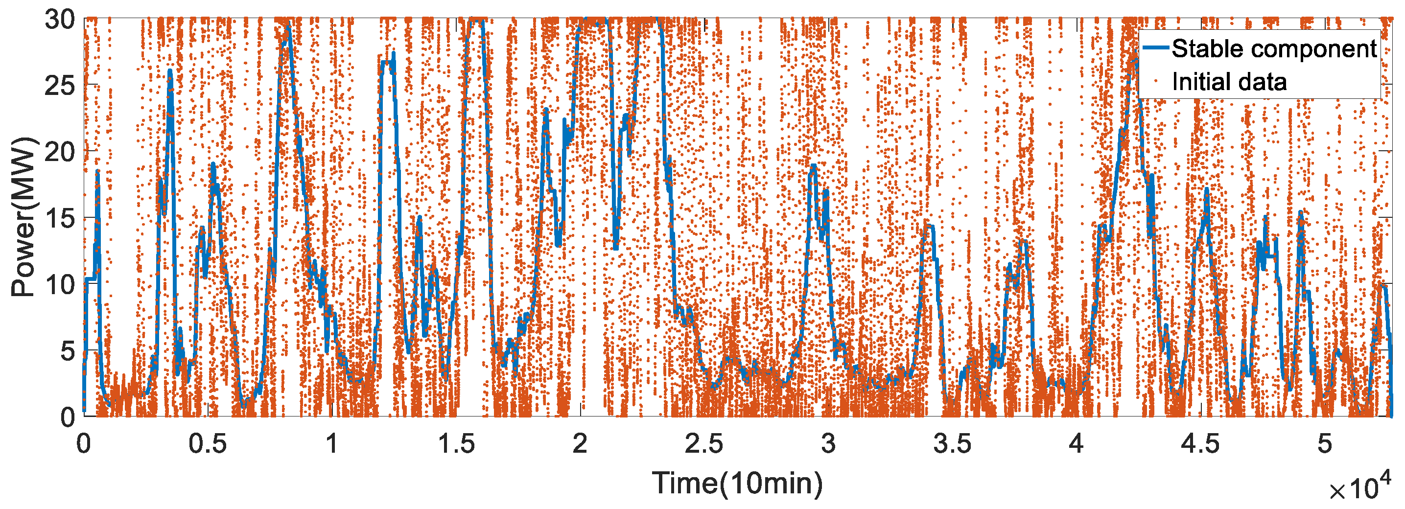
Figure 1 presents the distribution map of the historical annual mean wind power output of an actual wind farm. The wind power counts as zero if the wind velocity is lower than the cut-in speed or higher than the cut-off speed. The maximum output of the wind power system P_max is 30 MW and the sampling interval T_c is 10 min.

The stable component in Figure 1 is extracted through median filtering, which is expressed as

$$g(x)=\mathrm{med}\{f(x-k),k\in W\},$$

(1)

where f(x) and g(x) are initial wind power data and the stable component, respectively; med is the median filtering function [13], the fundamental purpose of which is to replace every element value of the data sequence by its median within a certain interval; and W = 1008 (±1) is the filter window.

Assuming that most of the stable component of the wind power output data within a week fluctuates narrowly around a certain median, the wind power fluctuation can be formulated by the pulsating component as follows:

$$P_{\mathrm{wav}}(t)=P_{\mathrm{int}}(t)-P_{\mathrm{ave}}(t),$$

(2)

where P_wav is the pulsating power component, P_int is the initial power output, and P_ave is the stable power component.

Equation (2) indicates that the pulsating power value of zero mean could be positive or negative, which is expressed as follows:

$$\{\begin{array}{l}{P}_{+}(i)=P_{\mathrm{wav}}(i),P_{\mathrm{wav}}(i)\ge 0,\\ P_{-}(i)=\left|P_{\mathrm{wav}}(i)\right|,P_{\mathrm{wav}}(i)\le 0,\\ i=1,2,\cdots ,M.\end{array}$$

(3)

Here, P₊ and P₋ are the positive and negative pulsating powers, respectively, and M = 52,560 is the sum of the sampling points over 365 days.

For the actual wind farm, the stable power represents the highest level of the acceptance ability of the grid for wind power. Thus, the positive pulsating power representing the excessive wind power should be chipped off, and the negative pulsating power representing the power shortage should be filled up [14,15,16].

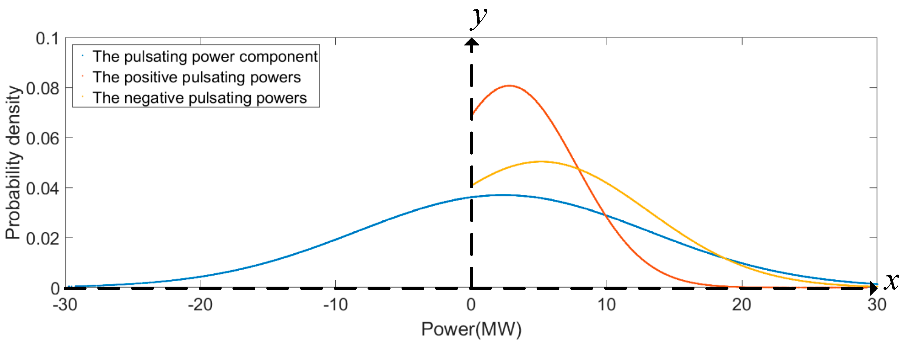
2.2. Probability Density Characteristics of Pulsating Power

Figure 2 presents the probability density curves of the pulsating power components. The PDF of the pulsating power component, as previously mentioned, obeys normal distribution, which is expressed as:

$$h_{P_{\mathrm{wav}}}(x)=\frac{1}{\sqrt{2\mathsf{\pi }}\mathsf{\sigma }}{e}^{-\frac{{(x-\mathsf{\mu })}^2}{2{\mathsf{\sigma }}^2}},$$

(4)

where σ is the standard deviation and μ is the mathematical expectation.

It can be seen from Figure 2 that the PDFs of the positive and negative pulsating power both obey a positively skewed distribution, and most of the power values are concentrated on the vertical axis side [17]. This is because the majority of the stable power component is equal to the initial power output.

In particular, the scale parameter σ and the location parameter μ are different between the positive and negative pulsating power when the initial wind power data is non-ideal, as shown in Figure 1. Here, the ideal wind power data refers to that in which the PDF obeys the standard normal distribution.

Qualitatively speaking, the amplitude distribution of the pulsating power is determined by σ, and the occurring probability of the pulsating power increases as the amplitude of variation decreases. Hence, the requirement of the frequency domain response of the energy storage system will depend on σ. On the other hand, the location of the maximum probability matching pulsating power is determined by μ, and the following discussion will focus on how to calculate the optimum energy storage capacity of the wind power system according to μ.

3. Rule of Planning the Energy Storage Capacity

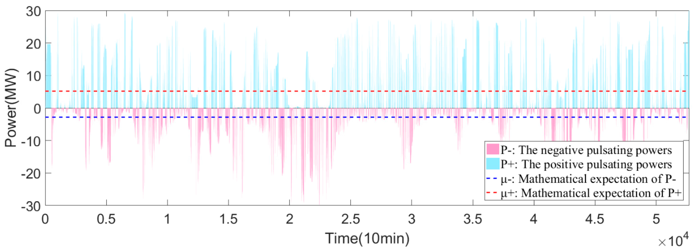
We define μ₊ and μ₋ as the mathematical expectations of P₊ and P₋, respectively. Figure 3 presents the distribution map of positive and negative pulsating power. Here, μ₊ is the optional value of the rated energy storage power and μ₋ is the absolute optional value of the rated compensation power.

The ideal wind power condition should manifest, in Figure 3, with the area enclosed by the horizontal axis and the curve of P₊ being equal to the area enclosed by the horizontal axis and the curve of P₋, indicating that the excessive wind energy is just enough to compensate for the wind energy shortage, and that the output waveform of the wind power agrees with the stable power component waveform. However, this has not happened in Figure 3 due to the stochastic nature of wind speed. Here, the horizontal line of μ₊ and μ₋ is not coincident, which is expressed as μ₊ ≠ |μ₋|.

3.1. Reference Value of the Energy Storage Power

To guarantee a long-term balance between energy supply and demand, the space of energy exchange between the storage equipment and the compensation equipment should be equal in size. Therefore, the choice of μ₊ or |μ₋| as the reference value of the energy storage power needs to be made. Furthermore, the choice will depend on the historical wind power condition [18,19,20], which is expressed as follows:

(1)

If μ₊ > |μ₋|, and the wind energy condition meets the formula:

$${\displaystyle \sum _{i=1}^{M_{+}}{P}_{+}(i)}>{\displaystyle \sum _{i=1}^{M_{-}}{P}_{-}(i)},$$

(5)

where M₊ and M₋ are the numbers of non-zero-valued sampling points of positive and negative pulsating power components, respectively, then μ₊ should be chosen. In this case, the wind energy is rich, but the excessive wind energy cannot be completely absorbed by the grid, even if the energy storage power is increased to |μ₋|.

(2)

If μ₊ < |μ₋|, and the wind energy condition meets the formula:

$${\displaystyle \sum _{i=1}^{M_{+}}{P}_{+}(i)}<{\displaystyle \sum _{i=1}^{M_{-}}{P}_{-}(i)},$$

(6)

then |μ₋| should be chosen. In this case, the wind energy is poor, and the accumulated wind energy cannot compensate for the wind power shortage for long even if the energy storage power is increased to μ₊.

In this paper, the wind farm power output fits Condition 1 and the reference value of the energy storage power is |μ₋|.

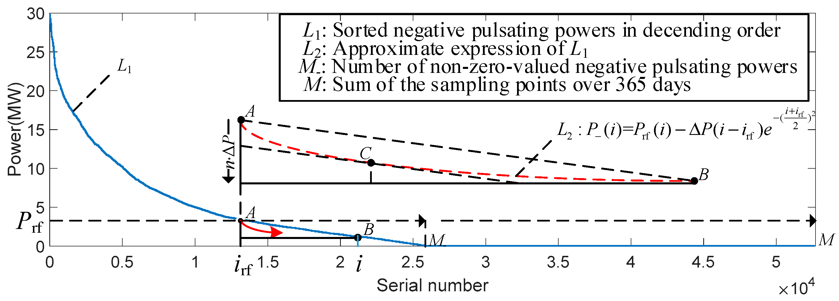
3.2. Approximate Expression of the Pulsating Power

Figure 4 presents the distribution map of the sorted negative pulsating power in descending order. The y-axis P_rf of point A represents the value of the reference power, and the x-axis i_rf represents the serial number of P_rf.

From Figure 2, we find that the probability density distribution of the sorted negative pulsating power, shown in Figure 4, becomes larger as the value of the sampling point approximates P_rf. It can be seen that there exists a mapping relation between the increment of the power value and the relative serial number.

We define ΔP as the minimum power increment, which represents the power regulation precision for the energy storage equipment. Obviously, the sampling point of the sorted power distributes more sparsely within the vertical power interval [P_rf − nΔP, P_rf] as the coefficient n is multiplied. Furthermore, the negative pulsating power at any sampling point i (i > i_rf | i ∈ M₋) can be formulated by P_rf, i_rf, and the weight function f(i) as follows:

$$\{\begin{array}{l}{P}_{-}(i)=P_{\mathrm{rf}}-n(i)\Delta P\\ n(i)=(i-i_{\mathrm{rf}})f(i)\end{array},i=i_{\mathrm{rf}}+1,i_{\mathrm{rf}}+2,\cdots ,M_{-}.$$

(7)

Here, P_rf and i_rf are known quantities, f(i) represents the slope variation of point C at which line L is tangential to the piece of curve P₋(i) between points A and B, and f(i) approximately obeys the exponential change law as described in Equation (4) as:

$$f(i)=e^{-\frac{1}{4}{(\frac{i-i_{\mathrm{rf}}}{M_{-}-i_{\mathrm{rf}}})}^2}.$$

(8)

Hence, the approximate expression of the pulsating power is given by Equations (7) and (8). There are two considerations for applying this expression:

(1)

When computing the energy storage power, the designed value is required to decrease along the red arrow in Figure 4 rather than the opposite. This is why the first serial number of independent variable i in Equation (7) is i_rf, and the power variation in the interval of i < i_rf is not expressed.

(2)

A calculation error exists in Equation (8). This is because the expression of P₋(i) is based on the assumptions that the part of curve P₋(i) between point A and point B obeys an exponential change law and that the x-axis of point C could be replaced by the middle coordinates of points A and B. The lower the concavity degree of P₋(i), the more likely the assumptions are to be true. Here, the precision of the approximate expression of the pulsating power can be quantitatively analyzed from the viewpoint of the probability distribution as follows [21].

We define ρ_ave as the average increment of the probability density, which represents the average range ability of the probability density of P₋(i) for each additional ΔP, and is expressed as:

$${\mathsf{\rho }}_{\mathrm{ave}}=\frac{h_{P_{-}}({\mathsf{\mu }}_{-})-h_{P_{-}}(P_{\max })}{M_{-}-i_{\mathrm{rf}}},$$

(9)

which represents the probability density corresponding to the maximum of the negative pulsating power, where $h_{P_{-}}(P_{\max })$ approaches zero for the actual wind farm.

According to Equation (9), the probability of the negative pulsating power value, which is calculated by Equations (7) and (8), being equal to its actual value can be formulated as:

$$\mathsf{\rho }(i)=1-(i-i_{\mathrm{rf}})\cdot {\mathsf{\rho }}_{\mathrm{ave}}.$$

(10)

We obtain from Equation (10) that the value of ρ(i) decreases when the difference between i and i_rf increases. However, there is no need to take the precision of the calculated negative pulsating power at the serial number of i, i >> i_rf, into consideration, because the actual value of P₋(i) will rapidly approach zero if i is close to M₋; meanwhile, the near-zero P₋(i) is useless for the energy storage capacity optimization to be described in the next subsection.

3.3. Energy Storage Capacity Optimization for Wind Power System

As is discussed in Section 3.1, |μ₋| is chosen to be the reference value of the energy storage power considering the actual wind energy conditions. In practice, the deployment of the energy storage power could be reduced so long as the pulsating power fluctuation of the wind farm is acceptable by the power grid, which is expressed as follows:

$$\{\begin{array}{l}{P}_{\mathrm{st}}=\left|\mathsf{\mu }-\right|-P_{-}(\mathsf{\lambda }{M}_{-})\\ \frac{i_{\mathrm{rf}}}{M_{-}}<\mathsf{\lambda }\le 1\end{array},$$

(11)

where P_st is the optimum energy storage power, P₋(λM₋) the lowest pulsating power, and λ is the probability assurance level that the sampling value of the pulsating power is higher than P₋(λM₋).

If λ = 1, then P_st = |μ₋|, indicating that the pulsating power fluctuation is maximally inhibited. Here, the fluctuation degree of the pulsating power, P_flu, can be formulated, if λ < 1, by the amplitude difference between the expectation of positive and negative pulsating power as follows:

$$P_{\mathrm{flu}}=\mathrm{hist}\{P_{\mathrm{ave}}+\{\begin{array}{l}{P}_{+},P_{+}<P_{\mathrm{st}}\\ P_{+}-P_{\mathrm{st}},P_{+}\ge P_{\mathrm{st}}\end{array}\},$$

(12)

where hist is the expectation function. Hence, the decreased percentage of P_flu compared to a wind power system without any energy storage equipment can be expressed as

$$\Delta P_{\mathrm{flu}}\%=(1-\frac{P_{\mathrm{flu}}}{{\mathsf{\mu }}_{+}+\left|\mathsf{\mu }-\right|})\times 100\%.$$

(13)

By far, the optimum energy storage power for the wind power system is given in Equation (11), and the evaluation index of the fluctuation degree of the firm power is given in Equation (13). Generally speaking, it is acceptable that the wind power output fluctuates around the stable power level at 10% (λ = 0.9) for the grid. On this basis, the allocated daily energy storage capacity E_st of the wind-storage hybrid power system is given by

$$E_{\mathrm{st}}=\frac{24M-(\left|{\mathsf{\mu }}_{-}\right|-P_{-}(0.9M_{-}))}{M}.$$

(14)

4. Evaluation of the Firm Power Escalation

The application of energy storage technology is based on the conversion of different energy forms, which involves energy loss. Energy loss results because only part of the excessive wind energy is converted into electric power to compensate for the power deviation of the wind farm, which is expressed as:

$${\displaystyle {\int }_{T_c{M}_{+}}(P_{\mathrm{int}}(t)-P_{\ast })\mathrm{d}t=}\mathsf{\eta }{\displaystyle {\int }_{T_c{M}_{-}}(P_{\ast }-P_{\mathrm{int}}(t))\mathrm{d}t},$$

(15)

where P_* is the new stable component of the wind power after power regulation, and η is the energy conversion rate.

When analyzing how the firm power is affected by the energy conversion rate, the ideal assumption of the initial wind power data is satisfied, and the number of non-zero-valued sampling points of positive and negative pulsating power components are just equal, which is expressed as follows:

$$\{\begin{array}{l}{\displaystyle {\sum }_{M_{+}}{P}_{+}(i)}={\displaystyle {\sum }_{M_{-}}|P_{-}(i)|}\\ M_{+}=M_{-}\end{array}.$$

(16)

Substituting Equations (2), (3) and (16) into Equation (15) yields the relationship between the firm power of the wind farm and the conversion rate of the energy storage equipment as follows:

$$\frac{T_{\mathrm{c}}\cdot M_{-}\cdot P_{\ast }}{{\displaystyle {\int }_{T_{\mathrm{c}}{M}_{-}}{P}_{\mathrm{ave}}(t)dt}}=1+\frac{1-\mathsf{\eta }}{1+\mathsf{\eta }}\cdot \frac{{\displaystyle {\int }_{T_{\mathrm{c}}{M}_{-}}{P}_{-}(t)dt}}{{\displaystyle {\int }_{T_{\mathrm{c}}{M}_{-}}{P}_{\mathrm{ave}}(t)dt}}.$$

(17)

Here, the expected value of P_ave is the average sampling value of the initial wind power output data. Thus, Equation (17) could be simplified according to Equation (7) as follows:

$$\frac{P_{\ast }}{\widetilde{P_{\mathrm{ave}}}}=1-\frac{1-\mathsf{\eta }}{1+\mathsf{\eta }}\cdot (\frac{P_{\mathrm{rf}}}{\widetilde{P_{\mathrm{ave}}}}-p_{\mathsf{\lambda }}),$$

(18)

where $\widetilde{P_{\mathrm{ave}}}$ is the mean value of P_ave; p_λ is the pulsating power calculated by the given λ, ΔP, and M₋, which is formulated according to Equation (8) as:

$$p_{\mathsf{\lambda }}=\frac{-2{(M_{-}-i_{\mathrm{rf}})}^2}{M_{-}\cdot \widetilde{P_{\mathrm{ave}}}}(e^{-{(\frac{\mathsf{\lambda }{M}_{-}-i_{\mathrm{rf}}}{2(M_{-}-i_{\mathrm{rf}})})}^2}-e^{-{(\frac{i_{\mathrm{rf}}}{2(M_{-}-i_{\mathrm{rf}})})}^2}).$$

(19)

We define E_η as the percentage of the difference of the firm power escalation to its highest level, and we know from Equation (18) that, when energy loss exists, E_η is determined by P_rf, η, and λ, which is expressed as follows:

$$E_{\mathsf{\eta }}=(1-\frac{P_{\ast }}{\widetilde{P_{\mathrm{ave}}}})\times 100\%.$$

(20)

5. Simulation Results

To verify the proposed rule for computing the energy storage capacity and the evaluation method of the firm power escalation, the accuracy of the approximate expression of the pulsating power should be proven first. The parameters of the simulated wind-storage hybrid power system are listed in

Table 1. Parameters of the simulated wind- storage hybrid power system.

Variable	Description	Value	Unit
Prf	Reference value of the energy storage power	2.83	MW
irf	Serial number of Prf	14,952	—
M−	Number of non-zero sampling points of the negative pulsating power	26,031	—
ΔP	Power regulation precision of the energy storage equipment	0.26	kW

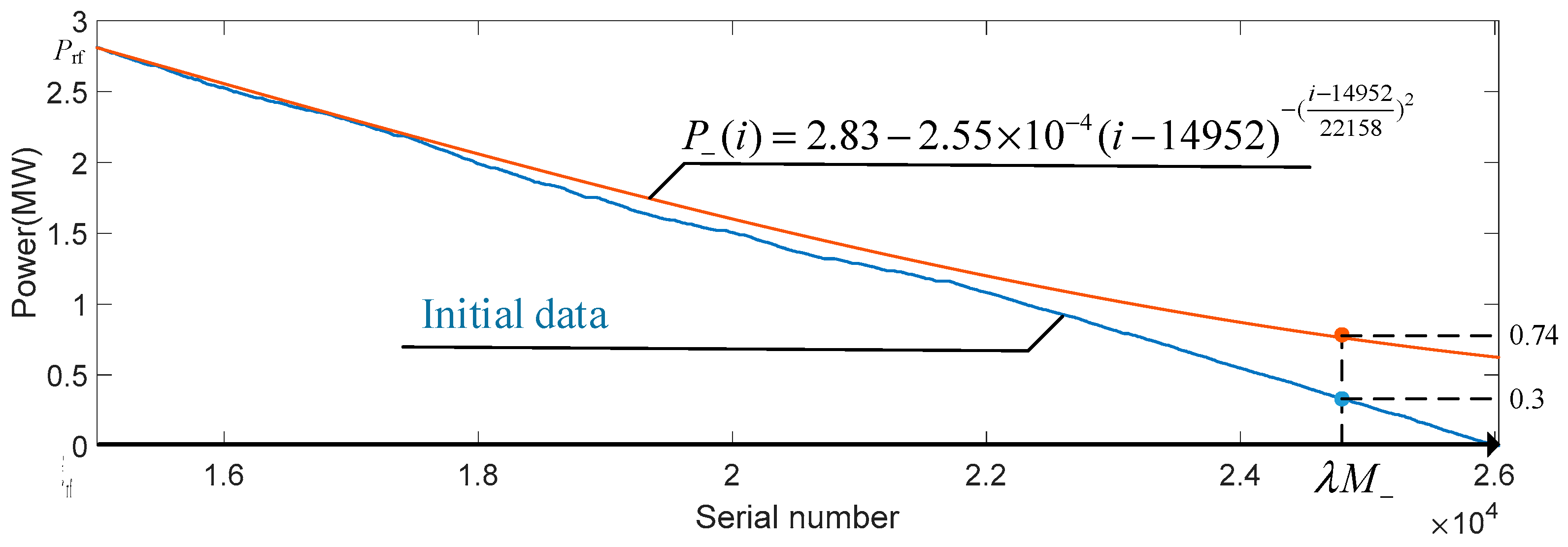
. Figure 5 shows the approximate curve of the non-zero negative pulsating power.

We note from Figure 5 that the difference between the calculated lowest pulsating power and its true value, when the probability assurance level is 90%, is 0.44 MW. Meanwhile, the relative error of the calculated optimum energy storage power is 17.4%. The probability distribution of the lowest negative pulsating power being equal to the true value is listed in

Table 2. Probability distribution of ρ(λ).

Variable	Description	Value
hp−(μ−)	The probability density corresponding to the expectation of the negative pulsating power	8%
hp−(Pmax)	The probability density corresponding to the maximum of the negative pulsating power	0
ρave	The range ability of the probability density of the negative pulsating power	7.2 × 10−6
ρ(λ = 0.9)	The range ability of the probability density of the negative pulsating power as λ equals 0.9	93.80%
ρ(λ = 0.8)	The range ability of the probability density of the negative pulsating power as λ equals 0.8	95.70%
ρ(λ = 0.7)	The range ability of the probability density of the negative pulsating power as λ equals 0.7	97.60%
ρ(λ = 0.6)	The range ability of the probability density of the negative pulsating power as λ equals 0.6	99.50%

.

From Table 2 we know that P₋(λM₋) increases and is more likely to approach the true value as λ decreases. The probability of P₋(λM₋), calculated by the approximate expression shown in Figure 5, being equal to the true value is 93.8%, which proves the high accuracy of the approximate expression.

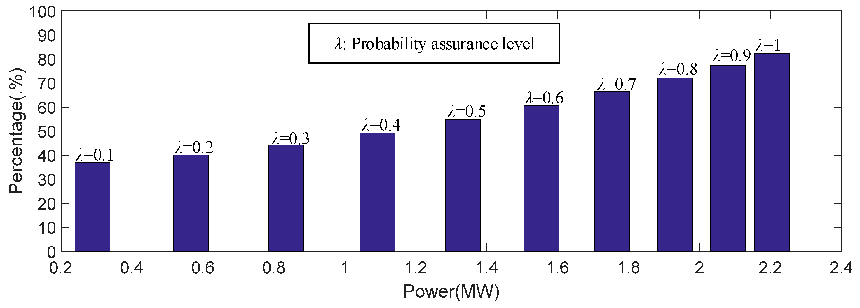
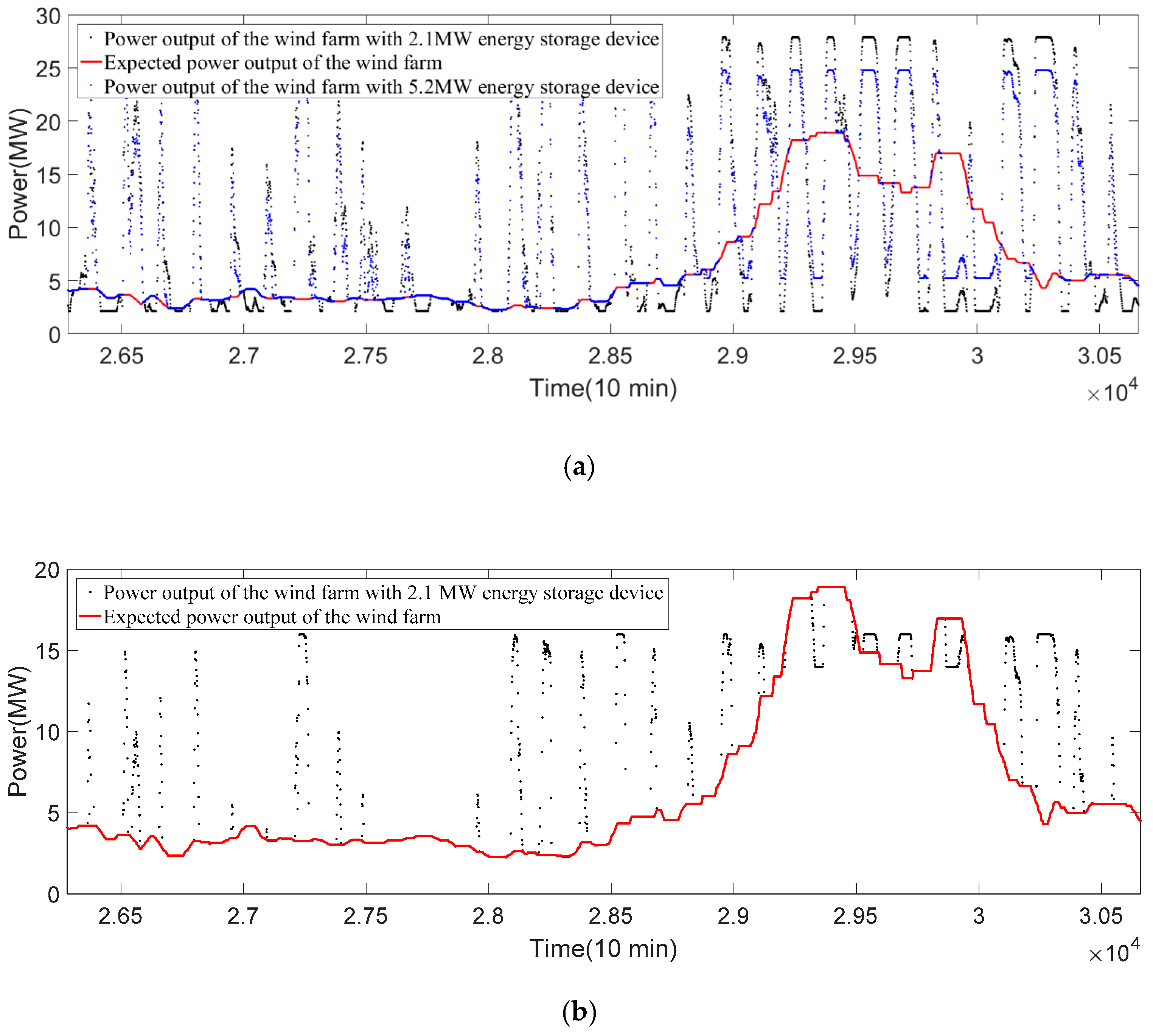
Figure 6 presents the tendency of ΔP_flu varying along with P_st. It can be seen that the amplitude of power fluctuation decreases as the deployment of the energy storage power increases. The decreased percentage of P_flu compared to a wind power system without any energy storage equipment is 77.3%, indicating that the stability of wind power output is improved. Here, the allocated energy storage power (optimum value) is 2.1 MW, and the daily energy storage capacity is 25.2 MWh.

To observe the power-regulating performance of the wind-storage hybrid power system, the output curves of the simulated wind farm output in June and December are presented in Figure 7a,b respectively. It can be seen from Figure 7a that the power output level of the wind farm is continuously higher than its expectation since there is plenty of excessive wind energy in June. This situation will be improved if the energy storage power is increased; for example, to the μ₊ of 5.2 MW. Furthermore, the operating mode of the wind turbines shall be adjusted to compensate for such predictable extreme wind conditions.

The power regulating system is shown to perform better in Figure 7b in comparison to Figure 7a. This is because the wind conditions in December approach the expectation level described in Section 3.1, and the monthly saved wind energy during that period is approximately 5600 MWh.

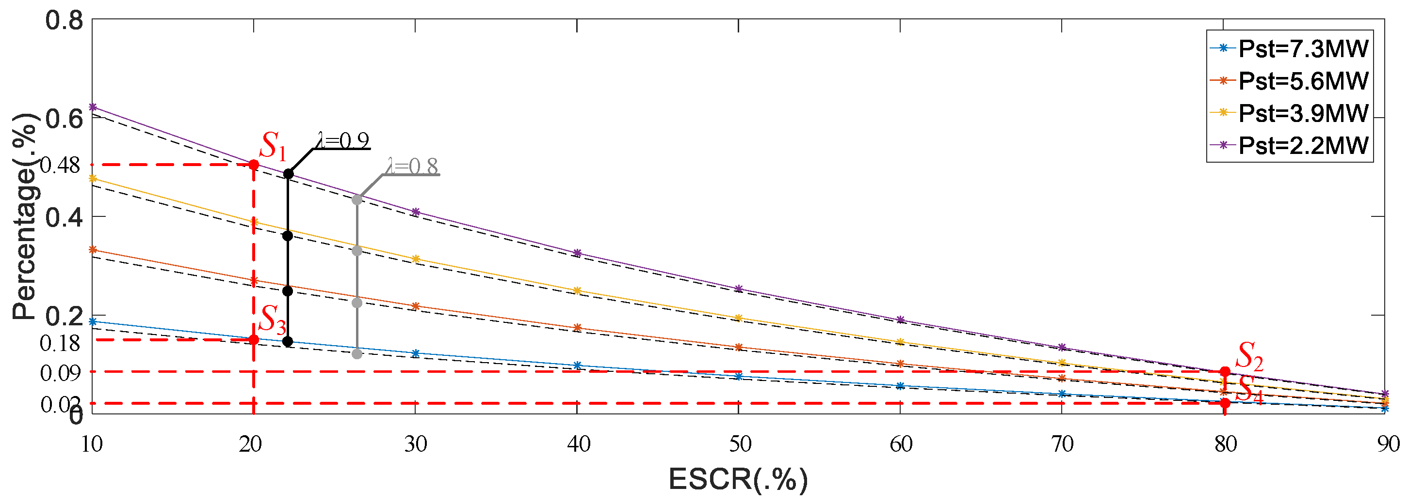
Figure 8 presents the relation curve of the evaluation index of the firm power escalation (EIFPE) with the energy storage power and the energy storage conversion rate (ESCR). It can be seen that the main influencing factors for the firm power are the energy storage power and the energy conversion rate, while the influence of the probability assurance level can be ignored. Furthermore, the negative impact of the decrement of the conversion rate on the firm power can be reduced by allocating a larger energy storage capacity.

Observing points S₁ and S₂ in Figure 8, the allocated energy storage power at both points is 2.1 MW. The difference in the percentage of the firm power escalation at its highest level is decreased from 49 to 9, and the amplitude of variation is 40%, as the energy storage conversion rate (ESCR) increases from 20% to 80%. Observing points S₃ and S₄, compared with the case of points S₁ and S₂, when the allocated energy storage power is increased from 2.1 to 7.3 MW, the difference in the percentage of the firm power escalation to its highest level is decreased from 18 to 2, and the amplitude of variation is decreased from 40% to 16% as the ESCR increases from 20% to 80%.

6. Conclusions

Although energy storage systems implement large-scale wind energy resources, a rule for planning the required storage space is pending. In this paper, the energy storage power and capacity are computed based on the pulsating component expectation of the historical annual mean wind power output data. The inhibited power output of a wind farm approaches the level of the stable power component and the utilization of the wind energy is maximized. In addition, the decrement percentage of the fluctuation degree of the pulsating power is chosen to be the evaluation index of the firm power escalation. On this basis, the scheme of reducing the energy storage power within the accepted range for the power grid is defined. After that, the relationship between the evaluation index and the technical parameters of the energy storage device, including the storage power, storage capacity, and the conversion rate, were quantitatively analyzed. To verify the performance of the proposed rule of planning the energy storage space and the evaluation method of the firm power escalation, simulation results have been demonstrated on the Matlab platform. The simulation results show that the firm power of a wind farm will be significantly escalated even if the conversion rate of the equipment is approximately 20% as long as the energy storage power is reasonable enough. Otherwise, if the allocated energy storage power of the wind farm is limited, the conversion rate of the energy storage equipment should be as high as possible.