Demand-Side Energy Management Based on Nonconvex Optimization in Smart Grid


1
School of Electrical Engineering, Yanshan University, Qinhuangdao 066004, China
2
Key Laboratory of System Control and Information Processing, Ministry of Education, Shanghai Jiao Tong University, Shanghai 200240, China
*
Author to whom correspondence should be addressed.
Energies 2017, 10(10), 1538; https://doi.org/10.3390/en10101538
Submission received: 7 September 2017
/
Revised: 23 September 2017
/
Accepted: 28 September 2017
/
Published: 4 October 2017
(This article belongs to the Special Issue Distributed Energy Resources Management)
Abstract
:Demand-side energy management is used for regulating the consumers’ energy usage in smart grid. With the guidance of the grid’s price policy, the consumers can change their energy consumption in response. The objective of this study is jointly optimizing the load status and electric supply, in order to make a tradeoff between the electric cost and the thermal comfort. The problem is formulated into a nonconvex optimization model. The multiplier method is used to solve the constrained optimization, and the objective function is transformed to the augmented Lagrangian function without constraints. Hence, the Powell direction acceleration method with advance and retreat is applied to solve the unconstrained optimization. Numerical results show that the proposed algorithm can achieve the balance between the electric supply and demand, and the optimization variables converge to the optimum.
1. Introduction
The power system includes generators, transformers, transmission, and distribution lines that deliver electricity power to terminal users. Smart grid enables real-time control and monitoring to provide distributed generation and storage. It can make grid operating reliably, economically and efficiently [1,2]. In smart grid, the energy providers can monitor the operating states of the loads in real time and control power supply directly. Demand-side energy management has been a hot topic in recent years [3,4]. Reasonable energy management can effectively promote the development of clean energy, save resources and reduce generation costs. In the process of the energy management, the consumers are encouraged to adjust the electricity purchase, optimize the load curve and improve the electricity efficiency [5,6,7]. Demand-side energy management is a mechanism which requires the consumers’ response to pricing strategy [8,9,10]. The real-time price is an effective strategy to achieve demand-side response [11,12,13].
In [14], an energy management service for the smart building has been proposed to measure and predict the patterns of both energy generation and power load. Taking into account overall costs, climatic comfort level and timeliness, a mixed integer linear programming model and a heuristic algorithm were proposed to make consumers change the consumption profile during certain time interval [15]. In [16], an automatic rule creation based on the knowledge extraction of a smart building was proposed to optimize the consumers’ electricity usage. In [17], the Lagrangian dual algorithm was employed to solve the nonconvex problem, and it came up with efficient demand response scheduling schemes. In [18], a complex telecommunication infrastructure was designed to manage the data exchange among the energy management system, generators, loads, and field sensors/actuators. In [19,20,21], the cost minimization of interactive consumers was studied based on the noncooperative game theory. The interaction between the consumers and energy provider was modeled with Stackelberg game theory [22,23,24]. Recently, convex optimization has been used for decreasing the consumers’ total cost. In [25], distributed primal-dual algorithms were used to adjust the energy consumption and the price. And the primal-dual algorithm was used to analyze the volatility of electricity markets when considering the uncertainty in the consumer’s value function [26]. In [27], an optimal and automatic residential energy consumption scheduling framework was proposed to provide the real-time price schedule to the consumers. In [28], the model of price response was established for the consumers with stochastic charging behaviors. In [29], a fully distributed control algorithm was proposed based on the saddle point dynamics and consensus protocols. In [30], the relationship between the operating states and energy consumption of the loads under forecast error was considered in an energy management problem. In the above studies, the cost functions of the consumers are assumed to be known in advance. However, the cost cannot be directly modeled when considering the comfort of the consumers and the operating state of the loads, such as the thermal comfort and the temperature settings of the heating, ventilation, and air conditioning (HVAC) systems.
In this study, we model energy management as a constrained optimization problem with non-convex objective function. And the Fanger thermal comfort cost which is unknown is included. The objective is to minimize the discomfort costs of the consumers and the generation costs of the providers. Meanwhile, it should keep balance between the consumers’ total power consumption and the total generation. Each consumer’s load operating state should be limited in upper and lower limits. Hence we propose an iterative algorithm to solve the optimization problem and study the influence of the tradeoff factor and the air conditioning’s energy efficient ratio on the energy management scheme.
The rest of the paper is organized as follows. The energy management problem is formulated in Section 2. The algorithm is proposed in Section 3. Section 4 applies the algorithm to the energy management of HVAC systems. The simulation results and analysis are given in Section 5, and conclusions are summarized in Section 6.
2. Problem Formulation
In the process of the demand-side management, we consider an power system consisting of m consumers that are served by an utility company, as shown in Figure 1. The utility company announces the retail price through forecasting the consumers’ power consumption. According to the announced price, the consumers can schedule the loads’ operations to reduce the costs.
We suppose that an power grid with m loads and n buses. The operating states of consumer i’s load () is , and the generation on bus i () is . The function denotes the consumer i’s discomfort cost caused by the load changes, and denotes the generating cost. And the function denotes the relationship between the energy consumption and the operating state. We suppose the lower limit and upper limit of the operating state of consumer i’s load is and . The energy management can be formulated as the following optimization problem:
where is the parameter to achieve the tradeoff between the consumers’ discomfort costs and the generating costs. The energy management problem is to minimize the costs of consumers and providers subject to the energy balance constraints and the operating state limits.
3. Iterative Algorithms
In this section, an iterative algorithm is proposed to solve the above optimization problem. The algorithm, which includes multiplier method, Powell direction acceleration method, advance and retreat method and golden section method, is described in Figure 2.
This iterative algorithm can solve the unknown and nonconvex optimization problem, and the specific algorithms are introduced as the following 4 parts.
Part 1: Multiplier Method
As a general constrained optimization problem, the constraints can be transformed to the objective. For the multiplier method, the constrained augmented Lagrange function can be established as:
where , and are Lagrange multipliers, especially is denoted as the retail price. The multipliers are updated by
The termination criterions are and , where is the termination error. And and are given by
The multiplier method includes 4 steps, as shown in Algorithm 1.
| Algorithm 1 The multiplier algorithm. |
| Initialization: |
|
| Iteration: |
|
Part 2: Powell Direction Acceleration Method
In this paper, the explicit comfort function is hard to formulate, and it’s impossible to take the derivative of an unknown objective function. Therefore, we consider a data-driven algorithm to solve the unconstrained optimization problem directly. The Powell direction acceleration method is one of the most effective data-driven methods. The basic idea of Powell method is to build the conjugated search direction in the next iteration by calculations from the previous iterations.
In the original Powell method, the new search direction will take place of the first component in the old direction vector. However, these new vectors could be linear dependent, and the optimum cannot be obtained. Hence we use the modified Powell method. The modified Powell method can judge whether the new search direction could be applied in the next iteration. If it cannot be applied, judge which direction in the original searching has the lowest objective value. Then let the new search direction replace the old one. In this way, the conjugated direction can be obtained.
In the ith iteration, set , , , and . Let be the search direction: . If and , replace with . Else keep the original directions. The specific algorithm is given in Algorithm 2.
| Algorithm 2 The Powell direction acceleration algorithm. |
| Initialization: |
|
| Iteration: |
|
Part 3: Advance and Retreat Method
Since the objective function is a multimodal and non-convex function, we should segment an unimodal interval before one-dimensional searching based on the specific advance and retreat algorithm, as shown in Algorithm 3.
| Algorithm 3 The advance and retreat algorithm. |
| Initialization: |
|
| Iteration: |
|
Part 4: Golden Section Method
After segmented the interval, the optimal step length is calculated by Golden Section method, as shown in Algorithm 4.
| Algorithm 4 The golden section algorithm. |
| Initialization: |
| The search interval: ; . |
| Iteration: |
|
Remark 1.
The convergence of the algorithm has been proved in [31]. In the optimization problem with multi-dimensional variable, a global optimal point in each dimension can be obtained during the iterations. However, we cannot guarantee that the optimal points of all variables can be searched simultaneously in the same iteration, and the solution should be a sub-optimal solution in the calculation.
4. Application to Energy Management of HVAC Systems
In this section, we apply the iterative algorithms to the energy management of HVAC systems. The discomfort of consumers are characterized by the Fanger thermal comfort model. In the research of professor P. O. Fanger from Denmark, the predicted mean vote (PMV) and the predicted percentage of dissatisfied (PPD) were proposed to describe the human body’s comfort and satisfaction of the thermal environment, respectively. The Fanger thermal comfort model considers the thermal resistance of clothing, degree of human activities, the air temperature, the air velocity, the mean radiant temperature, and the moisture in the atmosphere. The PMV denotes the human body’s hot and cold sensation, including seven grades: hot, warm, little warm, moderate, little cool, cool, cold. The corresponding values are: . In practice, different people could have different feelings in the same thermal environment. To describe this relationship, the PPD target was proposed in [32,33,34].
The mathematical expression of PMV is denoted as:
where
and
where .
The PPD target represents a percentage of the human’s dissatisfaction of the environment, and the mathematical expression is given as:
The explanation of the parameters is shown in Table 1, and the relationship between PPD and PMV is shown in Figure 3.
We can build the following function to describe the consumers’ discomfort costs:
where is a constant coefficient that transforms the PPD to the discomfort cost. The generating cost of the provider is given as [35]:
where , , and are cost coefficients, which are determined by the power generation.
In the HVAC system, the relationship between the energy consumption and temperature is complicated. It could be influenced by many factors. For example, the cooling load includes the transmission load, the infiltration load, the solar load, and the internal load. The transmission load is the temperature transfer from outdoor to indoor through the components. The infiltration load is caused from the inflow of the air. The solar load is caused from the solar radiation. And the internal load is from the heat release of light, people and other electrical equipments [36], as shown in Figure 4.
The transmission load is denoted as:
where is the transmission load, is outdoor temperature, is the transfer constant in W/(°C), and is the transmission area.
The infiltration load is calculated as:
where is the infiltration load, is specific heat of air, is the air density, and is the volumetric air velocity and satisfies:
where is the effective infiltration area. and are determined by the wind speed and outdoor temperature. is the hight of the building.
The solar load and internal load are independent of the actual temperature settings and can be denoted as .
The total cooling load can be obtained:
In the HVAC system, the relationship between the cooling load and energy consumption is:
where is the coefficient determined by the transformation from the cooling load to the energy consumption.
The relationship between temperature settings and energy consumption can be formulated as:
where , , and .
Above all, the energy management model for the HVAC systems can be described as following optimization problem:
where is the indoor temperature. Each consumer’s temperature setting is limited by , where and are the minimal and maximal temperature settings, respectively.
5. Simulation Results
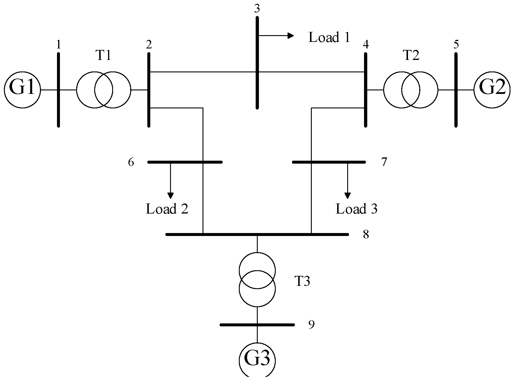
We consider two types of power systems that are installed with HVAC systems, e.g., the IEEE 9-bus system and IEEE 14-bus system shown in Figure 5 and Figure 6, respectively. The equality constraints in the IEEE 9-bus system and IEEE 14-bus system are and , respectively.
The parameter settings are shown in Table 2 [36], and the lower limit and the upper limit of the temperature setting for each consumer are 23 °C and 28 °C, respectively.
An important parameter of the HVAC system is energy efficiency ratio (EER). EER is the ratio of the actual cooling capacity to the actual input power during the cooling operation of the HVAC system, and the more efficient and power-saving HVAC has the higher EER. The EER is defined as , which is the reciprocal of in Equation (14).
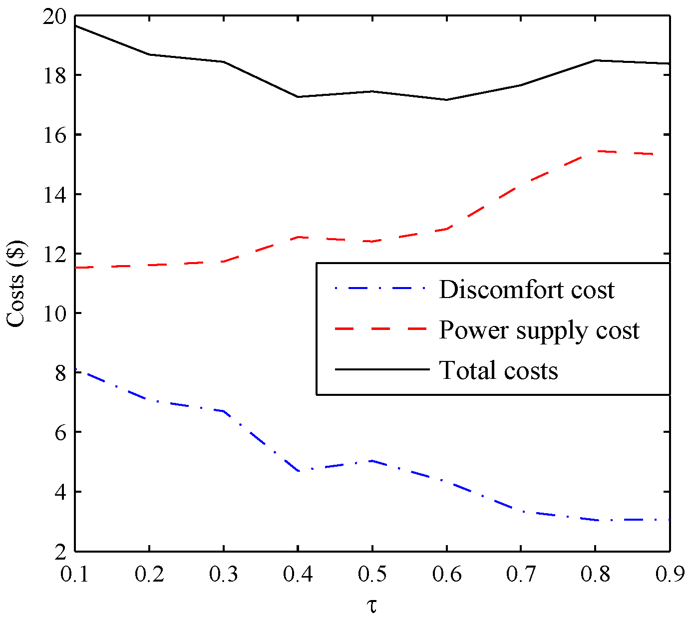
Taking the IEEE 9-bus system as an example, we discuss the impact of the tradeoff factor on the discomfort costs and power supply costs as well as the total costs. The results are given in Figure 7, from which, we can observe that the discomfort costs decrease with , and the generation costs increase with . When , we can obtain the minimum total costs. The parameter can achieve the tradeoff between consumers’ discomfort costs and providers’ generation costs. We can get minimum total costs through changing . The data of costs are shown in Table 3.
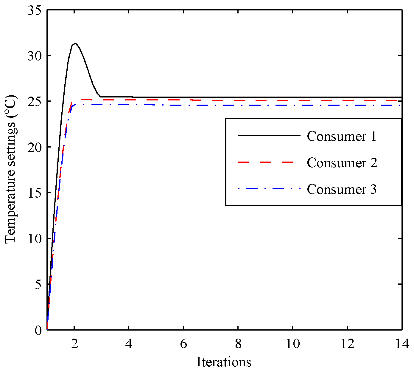
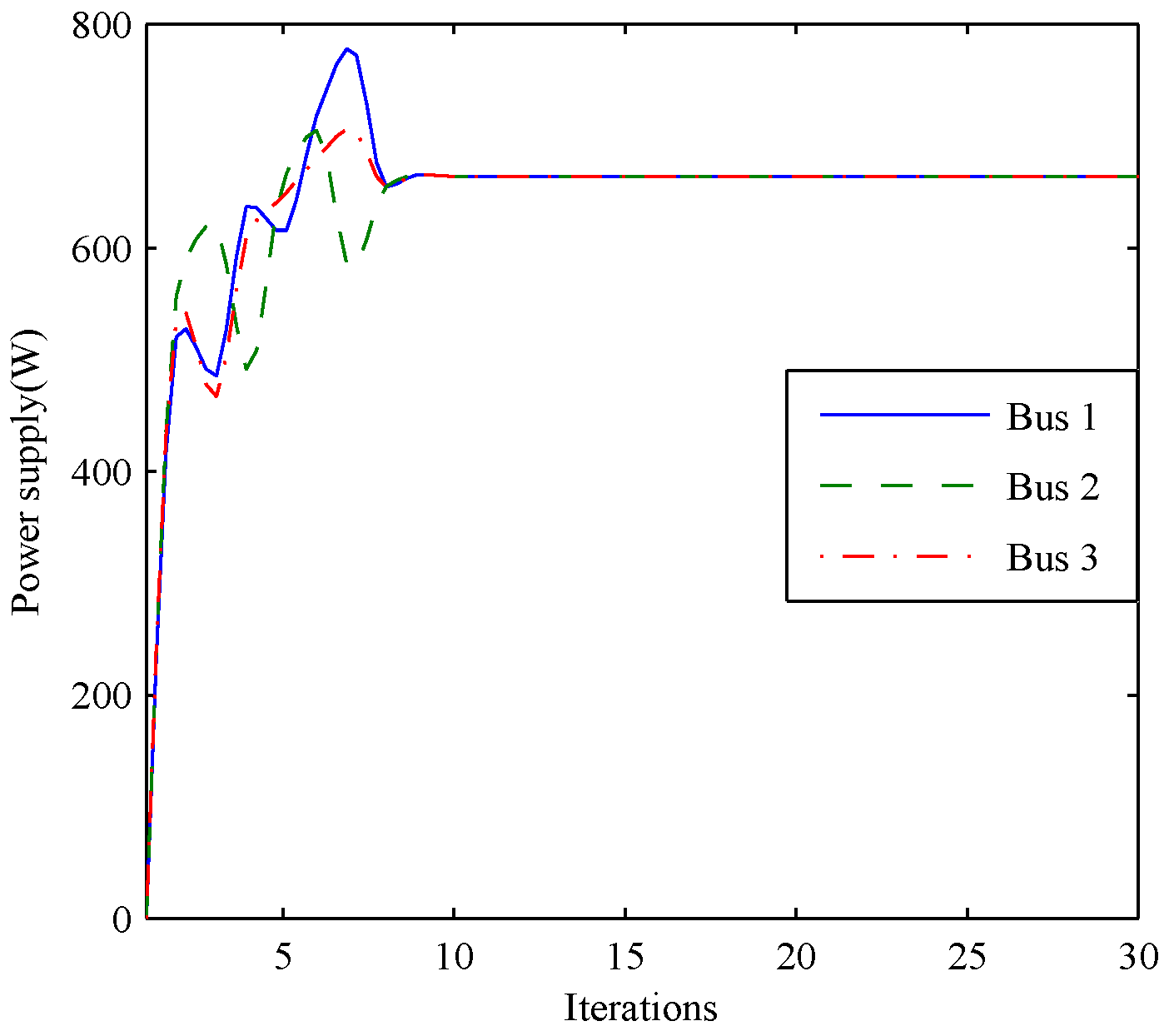
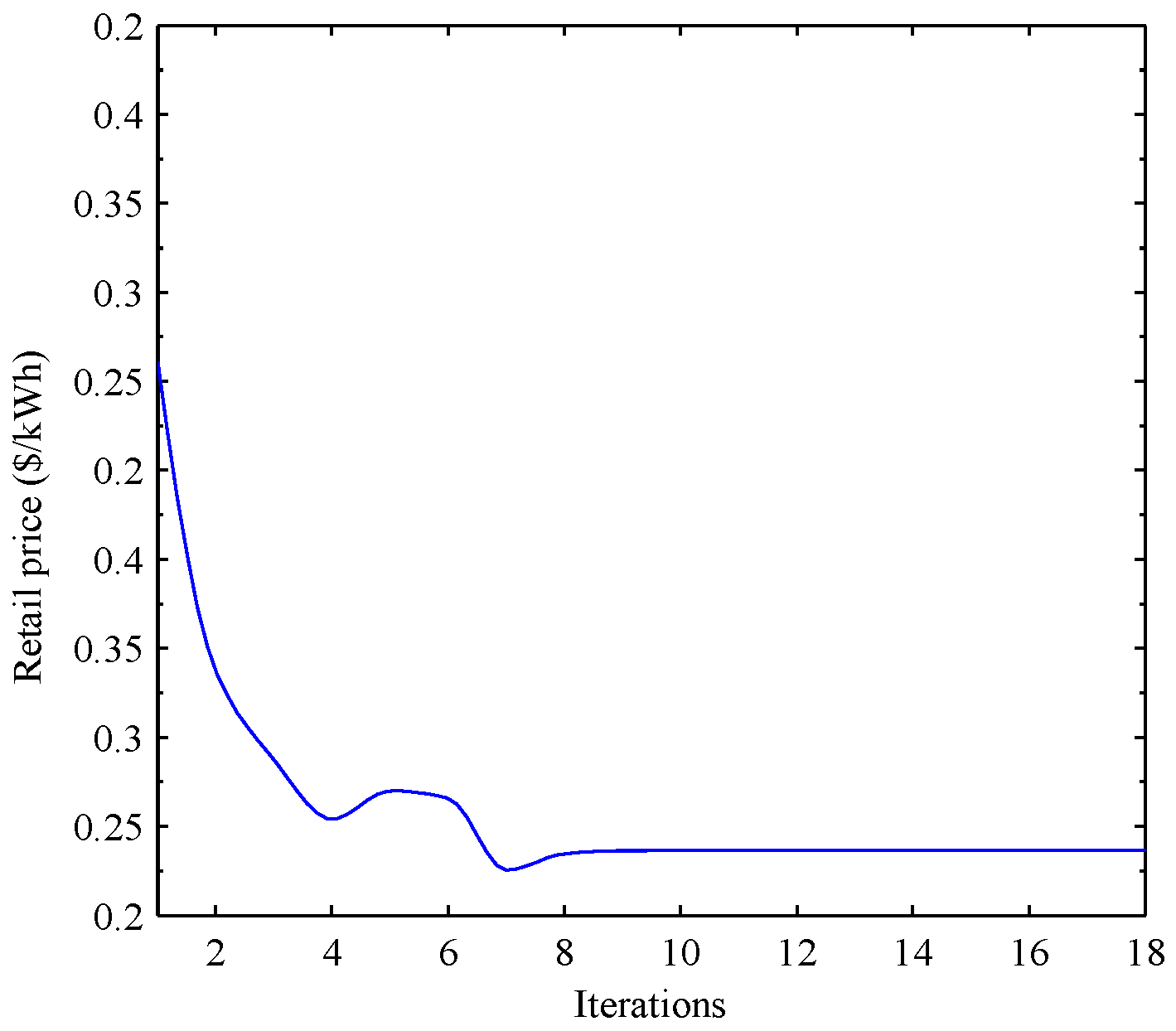
Next, we assume and evaluate the temperature settings, the power supply, and the retail price. The convergence of the temperature settings, the power supply, and the retail price are shown in Figure 8, Figure 9 and Figure 10, respectively.
According to Figure 8, Figure 9 and Figure 10, we can observe that all the optimization variables tend to be stable with the iterations and finally converge to the optimum.
It is observed from Table 4 and Table 5 that the temperature settings satisfy the requirements for upper limits and lower limits. And the total Power consumption is equal to the power supply. Moreover, the retail price is 0.2147 $/kWh, and the multipliers and are both zero. It means that the penalty terms are inactive at the optimum.
Next, we apply the energy management algorithm to the IEEE 14-bus system. It is observed from Figure 11, Figure 12 and Figure 13 that the temperature settings, the power supply and the retail price can converge to the optimum in the IEEE 14-bus system. Comparing with the convergence results in the IEEE 9-bus system, more iterations are needed. Furthermore, the power supply on each bus is more than IEEE 9-bus system, as shown in Table 6 and Table 7.
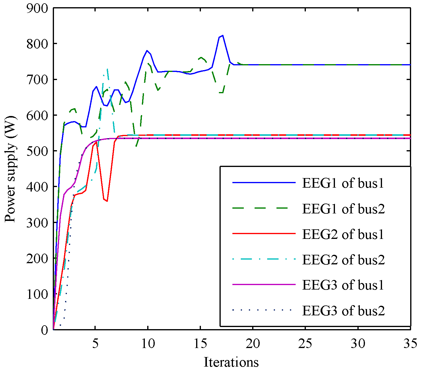
Next, we will discuss the effect of EER on the energy management system. We take three different energy efficiency grades (EEGs) of the HVAC systems: EEG 1, EEG 2, and EEG 3. The corresponding EERs are 3.5, 3.3, and 3.1, respectively. From Figure 14, we can observe that the higher EEG can cause lower retail price. Figure 15 shows that the lower EEG is effective in saving power consumption and the cost. It shows that the energy management algorithm motivates the consumers to use more energy-efficient HVAC.
6. Conclusions
This work studies a demand-side energy management problem based on the nonconvex optimization algorithm. The objective is to minimize the discomfort costs and the generation costs by changing the operating states of the loads and the power supply. Specially, the discomfort costs are formulated based on the Fanger thermal comfort. The nonconvex algorithm includes the multiplier method, the Powell method, the advance and retreat method, and the golden section method. One of the major advantages of this algorithm is that it can be applied in solving the unknown objective function caused by the thermal comfort model. In the simulation, we analyze the influence of the tradeoff factor and the EER on the energy management. It is observed that the minimum costs can be achieved by changing the value of , and different EERs can cause different retail prices and power consumption using the proposed energy management algorithm. The simulation results also demonstrate the convergence of the iterative algorithm and the balance between the power supply and power consumption.
Acknowledgments
This research was supported in part by National Natural Science Foundation of China under Grants 61573303 and 61503324, in part by Natural Science Foundation of Hebei Province under Grant F2016203438, E2017203284, and E2016203092, in part by Project Funded by China Postdoctoral Science Foundation under Grant 2015M570233 and 2016M601282, in part by Project Funded by Hebei Education Department under Grant BJ2016052, in part by Technology Foundation for Selected Overseas Chinese Scholar under Grant C2015003052, and in part by a Project Funded by Key Laboratory of System Control and Information Processing of Ministry of Education under Grant Scip201604.
Author Contributions
Kai Ma contributed the idea and wrote the paper; Yege Bai performed the experiments; Jie Yang designed the experiments; Yangqing Yu analyzed the data; Qiuxia Yang contributed the analysis tools.
Conflicts of Interest
The authors declare no conflict of interest.
Abbreviations
The following abbreviations are used in this manuscript:
| HVAC | Heating, Ventilation, and Air Conditioning |
| EER | Energy Efficient Ratio |
| EEG | Energy Efficient Grade |
| PHR | Powell-Hestenes-Rockafellar |
| PMV | Predicted Mean Vote |
| PPD | Predicted Percentage of Dissatisfied |
References
- Zaballos, A.; Vallejo, A.; Selga, J.M. Heterogeneous communication architecture for the smart grid. IEEE Netw. 2011, 25, 30–37. [Google Scholar] [CrossRef]
- Yu, Y.X.; Luan, W.P. Smart grid and its implementations. Proc. CSEE 2009, 29, 1–8. [Google Scholar]
- Elaiw, A.M.; Xia, X.; Shehata, A.M. Hybrid DE-SQP and hybrid PSO-SQP methods for solving dynamic economic emission dispatch problem with valve-point effects. Electr. Power Syst. Res. 2013, 103, 192–200. [Google Scholar] [CrossRef]
- Verschae, R.; Kato, T.; Matsuyama, T. Energy Management in Prosumer Communities: A Coordinated Approach. Energies 2016, 9, 562. [Google Scholar] [CrossRef]
- Divshali, P.H.; Choi, B. Electrical Market Management Considering Power System Constraints in Smart Distribution Grids. Energies 2016, 9, 405. [Google Scholar] [CrossRef]
- Gao, B.; Liu, X.; Zhang, W.; Tang, Y. Autonomous Household Energy Management Based on a Double Cooperative Game Approach in the Smart Grid. Energies 2015, 8, 7326–7343. [Google Scholar] [CrossRef]
- Miceli, R. Energy Management and Smart Grids. Energies 2013, 6, 2262–2290. [Google Scholar] [CrossRef] [Green Version]
- Albadi, M.H.; El-Saadany, E.F. A summary of demand response in electricity markets. Electr. Power Syst. Res. 2008, 78, 1989–1996. [Google Scholar] [CrossRef]
- Zhao, H.T.; Zhu, Z.Z.; Yu, E.K. Study on demand response markets and programs in electricity markets. Power Syst. Technol. 2010, 34, 146–153. [Google Scholar]
- Ma, K.; Liu, X.; Yang, J.; Liu, Z.; Yuan, Y. Optimal Power Allocation for a Relaying-Based Cognitive Radio Network in a Smart Grid. Energies 2017, 10, 909. [Google Scholar] [CrossRef]
- Mathieu, J.L.; Koch, S.; Callaway, D.S. State Estimation and Control of Electric Loads to Manage Real-Time Energy Imbalance. IEEE Trans. Power Syst. 2013, 28, 430–440. [Google Scholar] [CrossRef]
- Zhou, M.H.; Min, X.U. Researches on spot price based on optimal power flow and its algorithm. Relay 2006, 34, 63–67. [Google Scholar]
- Sanduleac, M.; Lipari, G.; Monti, A.; Voulkidis, A.; Zanetto, G.; Corsi, A.; Toma, L.; Fiorentino, G.; Federenciuc, D. Next Generation Real-Time Smart Meters for ICT Based Assessment of Grid Data Inconsistencies. Energies 2017, 10, 857. [Google Scholar] [CrossRef]
- Rottondi, C.; Duchon, M.; Koss, D.; Palamarciuc, A.; Pití, A.; Verticale, G.; Schätz, B. An Energy Management Service for the Smart Office. Energies 2015, 8, 11667–11684. [Google Scholar] [CrossRef] [Green Version]
- Agnetis, A.; de Pascale, G.; Detti, P.; Vicino, A. Load Scheduling for Household Energy Consumption Optimization. IEEE Trans. Smart Grid 2013, 4, 2364–2373. [Google Scholar] [CrossRef]
- Gupta, P.K.; Gibtner, A.K.; Duchon, M.; Koss, D.; Schätz, B. Using knowledge discovery for autonomous decision making in smart grid nodes. In Proceedings of the IEEE International Conference on Industrial Technology, Seville, Spain, 17–19 March 2015; pp. 3134–3139. [Google Scholar]
- Gatsis, N.; Giannakis, G.B. Residential demand response with interruptible tasks: Duality and algorithms. In Proceedings of the 2011 50th IEEE Conference on Decision and Control and European Control Conference, Orlando, FL, USA, 12–15 Dcember 2011; pp. 1–6. [Google Scholar]
- Barbato, A.; Bolchini, C.; Geronazzo, A.; Quintarelli, E.; Palamarciuc, A.; Pitì, A.; Rottondi, C.; Verticale, G. Energy Optimization and Management of Demand Response Interactions in a Smart Campus. Energies 2016, 9, 398. [Google Scholar] [CrossRef] [Green Version]
- Ma, K.; Hu, G.; Spanos, C.J. Distributed Energy Consumption Control via Real-Time Pricing Feedback in Smart Grid. IEEE Trans. Control Syst. Technol. 2014, 22, 1907–1914. [Google Scholar]
- Mohsenian-Rad, A.H.; Wong, V.W.S.; Jatskevich, J.; Schober, R.; Leon-Garcia, A. Autonomous Demand-Side Management Based on Game-Theoretic Energy Consumption Scheduling for the Future Smart Grid. IEEE Trans. Smart Grid 2010, 1, 320–331. [Google Scholar] [CrossRef]
- Deng, R.; Yang, Z.; Chen, J.; Asr, N.R.; Chow, M.Y. Residential Energy Consumption Scheduling: A Coupled-Constraint Game Approach. IEEE Trans. Smart Grid 2014, 5, 1340–1350. [Google Scholar] [CrossRef]
- Chai, B.; Chen, J.; Yang, Z.; Zhang, Y. Demand Response Management with Multiple Utility Companies: A Two-Level Game Approach. IEEE Trans. Smart Grid 2014, 5, 722–731. [Google Scholar] [CrossRef]
- Chen, J.; Yang, B.; Guan, X. Optimal demand response scheduling with Stackelberg game approach under load uncertainty for smart grid. In Proceedings of the IEEE Third International Conference on Smart Grid Communications, Tainan, Taiwan, 5–8 November 2012; pp. 546–551. [Google Scholar]
- Tushar, W.; Chai, B.; Yuen, C.; Smith, D.B. Three-Party Energy Management With Distributed Energy Resources in Smart Grid. IEEE Trans. Ind. Electron. 2014, 62, 2487–2498. [Google Scholar] [CrossRef]
- Samadi, P.; Mohsenian-Rad, A.H.; Schober, R.; Wong, V.W.S.; Jatskevich, J. Optimal Real-Time Pricing Algorithm Based on Utility Maximization for Smart Grid. In Proceedings of the First IEEE International Conference on Smart Grid Communications, Gaithersburg, MD, USA, 4–6 October 2010; pp. 415–420. [Google Scholar]
- Roozbehani, M.; Dahleh, M.A.; Mitter, S.K. Volatility of Power Grids Under Real-Time Pricing. IEEE Trans. Power Syst. 2011, 27, 1926–1940. [Google Scholar] [CrossRef]
- Mohsenian-Rad, A.H.; Leon-Garcia, A. Optimal Residential Load Control With Price Prediction in Real-Time Electricity Pricing Environments. IEEE Trans. Smart Grid 2010, 1, 120–133. [Google Scholar] [CrossRef]
- Soltani, N.Y.; Kim, S.J.; Giannakis, G.B. Real-Time Load Elasticity Tracking and Pricing for Electric Vehicle Charging. IEEE Trans. Smart Grid 2015, 6, 1303–1313. [Google Scholar] [CrossRef]
- Bai, L.; Ye, M.; Sun, C.; Hu, G. Distributed control for economic dispatch via saddle point dynamics and consensus algorithms. In Proceedings of the IEEE Conference on Decision and Control, Las Vegas, NV, USA, 12–14 Dcember 2016; pp. 6934–6939. [Google Scholar]
- Ma, K.; Hu, G.; Spanos, C.J. Energy Management Considering Load Operations and Forecast Errors with Application to HVAC Systems. IEEE Trans. Smart Grid 2016, PP, 1–10. [Google Scholar] [CrossRef]
- Sun, W.; Yuan, Y.X. Optimization Theory and Methods—Nonlinear Programming; Springer: New York, NY, USA, 2006; Volume 1. [Google Scholar]
- Van, H.J. Forty years of Fanger’s model of thermal comfort: Comfort for all? Indoor Air 2008, 18, 182–201. [Google Scholar]
- De Donato, S.R.; Graziani, M.; Mainetti, S. Evaluation of the predictive value of Fanger’s PMV index study in a population of school children. Predicted mean vote. Med. Lav. 1996, 87, 51. [Google Scholar] [PubMed]
- Gilani, I.U.H.; Khan, M.H.; Ali, M. Revisiting Fanger’s thermal comfort model using mean blood pressure as a bio-marker: An experimental investigation. Appl. Therm. Eng. 2016, 109, 35–43. [Google Scholar] [CrossRef]
- Wood, A.J.; Wollenberg, B. 96/02779—Power generation operation and control, 2nd edition. IEEE Power Energy Mag. 1996, 37, 90–93. [Google Scholar]
- Wang, N.; Zhang, J.; Xia, X. Energy consumption of air conditioners at different temperature set points. Energy Build. 2013, 65, 412–418. [Google Scholar] [CrossRef]
Figure 1.
Demand-side management system.
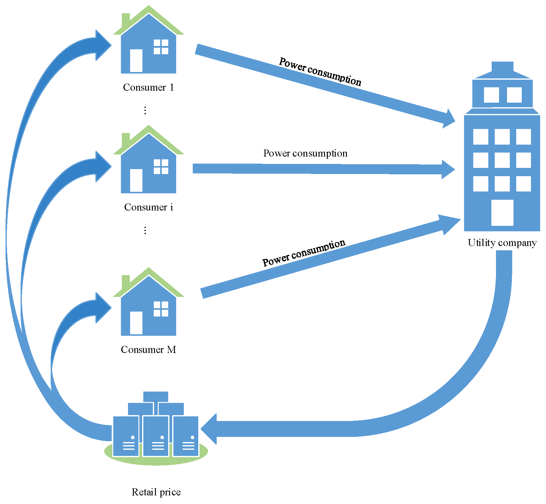
Figure 2.
The flowchart of the iterative algorithm.
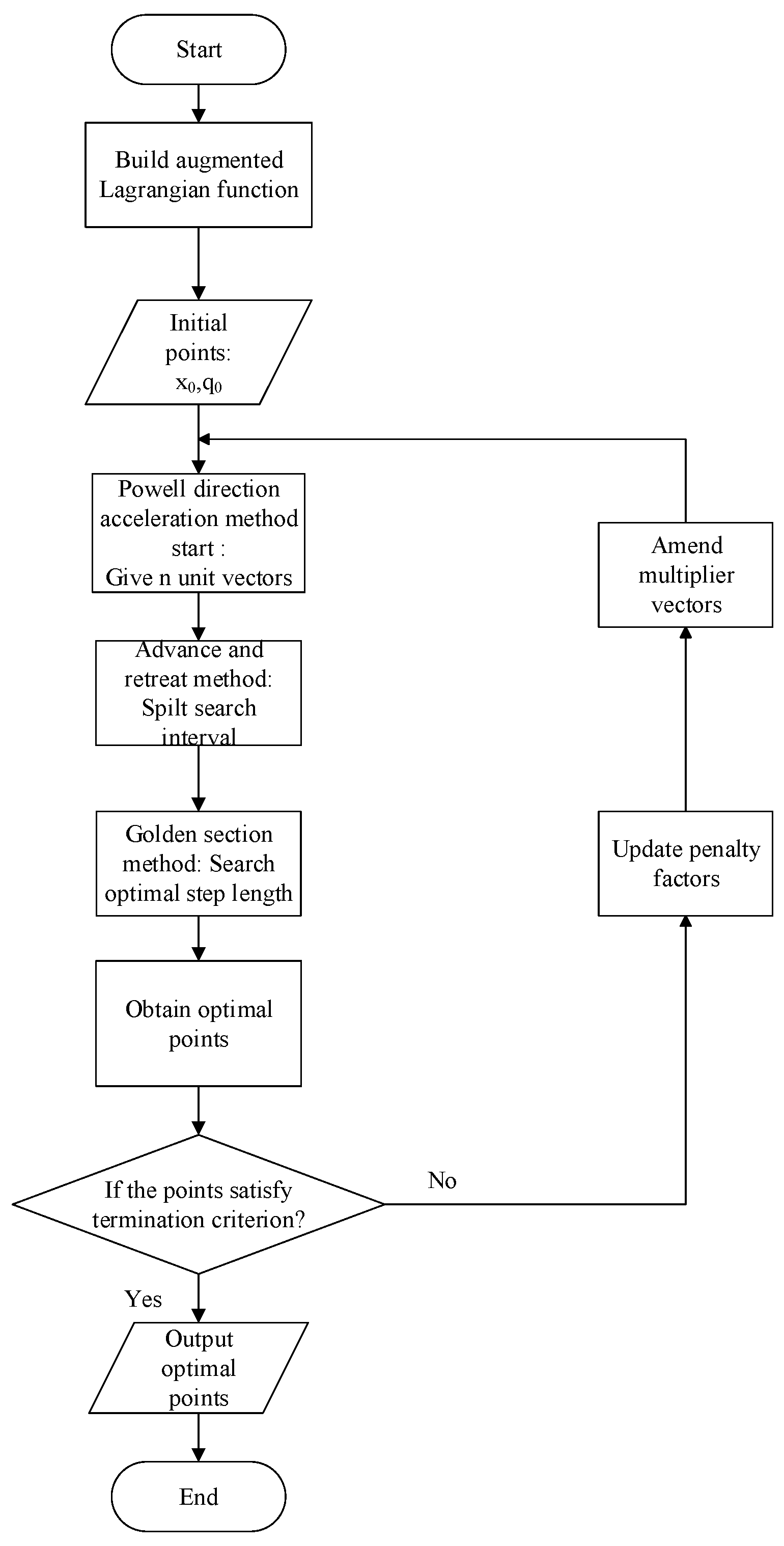
Figure 3.
The relationship between PPD and PMV.
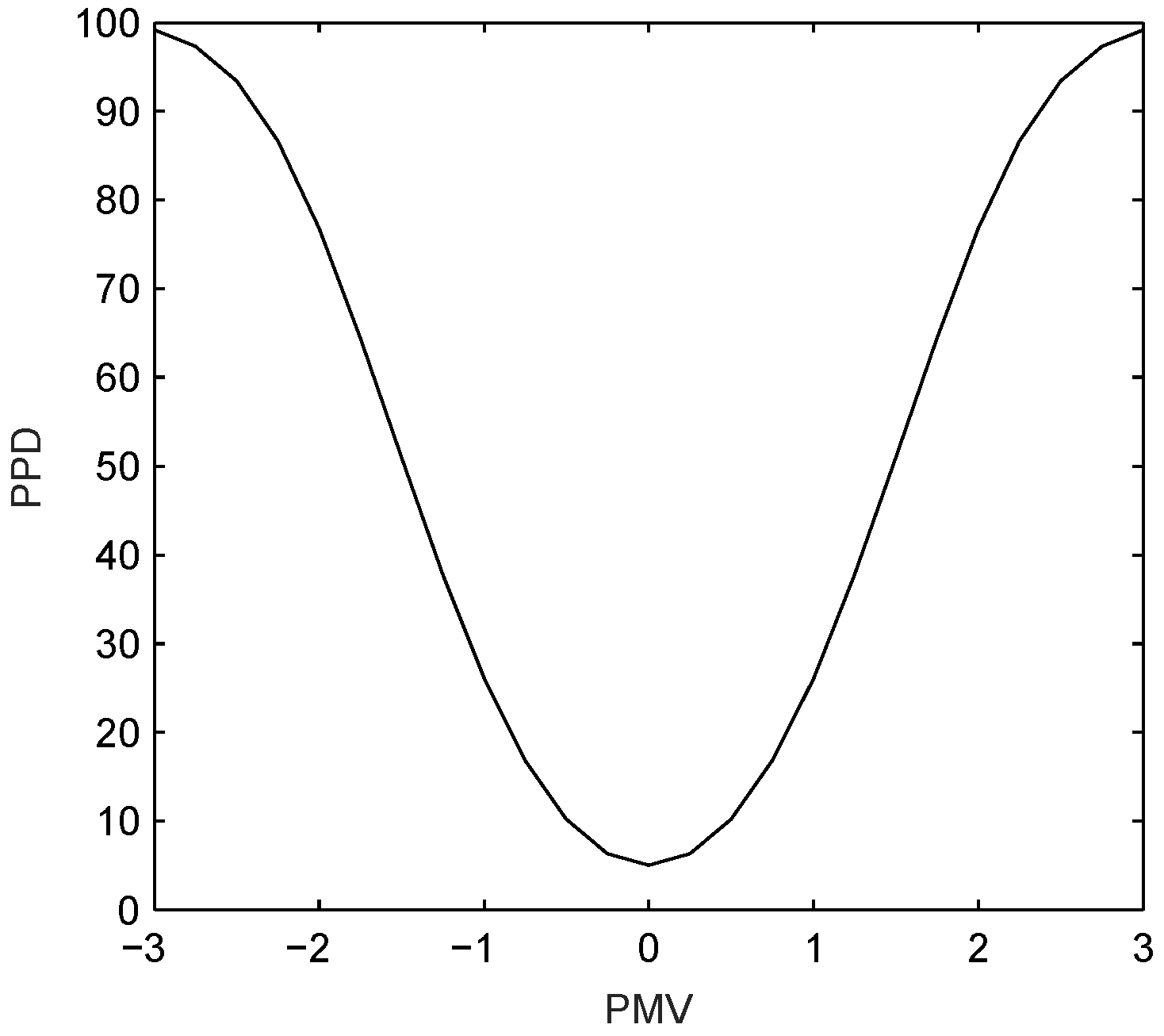
Figure 4.
The cooling load system.
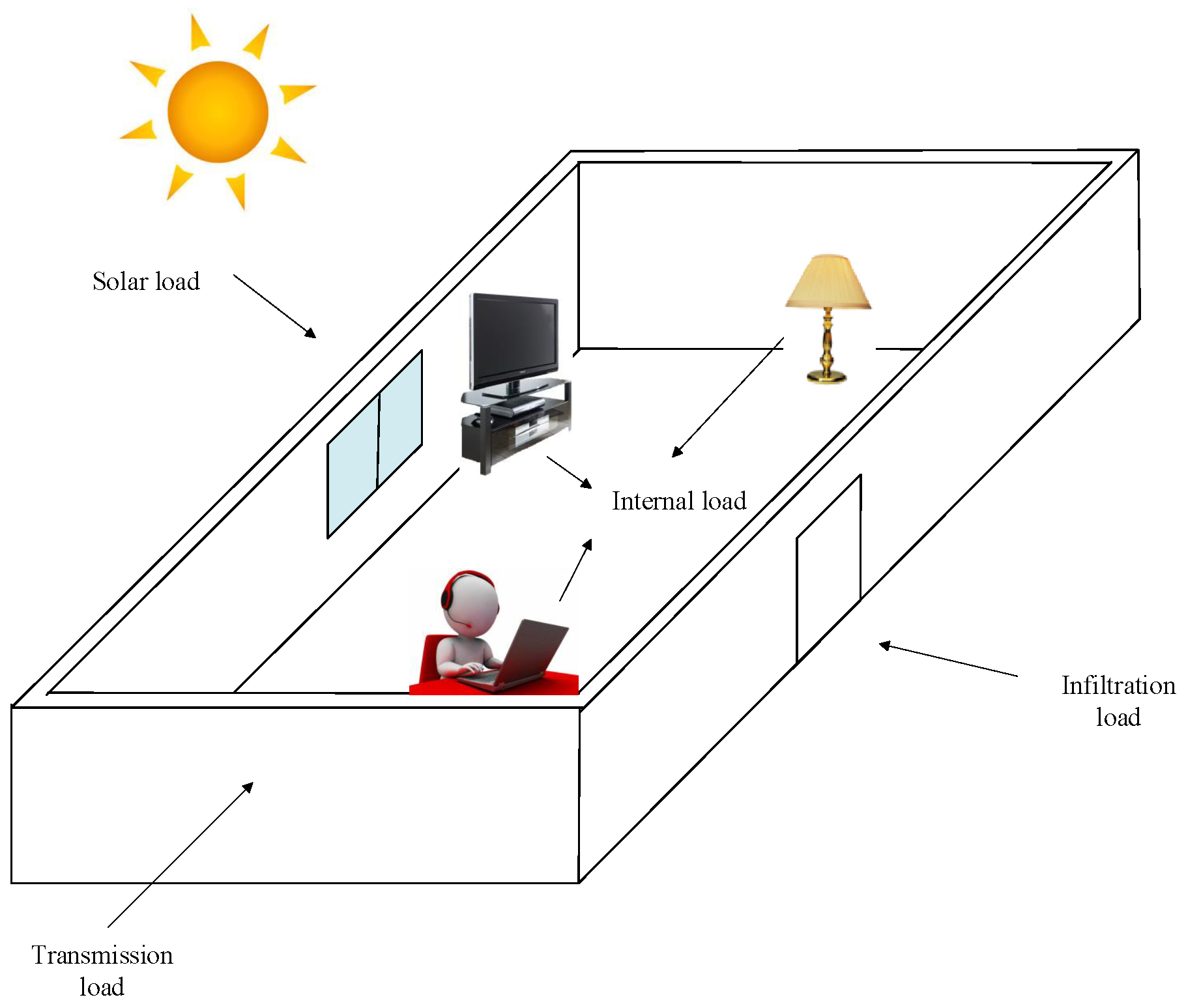
Figure 5.
IEEE 9-bus system: 9 buses, 3 generators, and 3 loads (, ).

Figure 6.
IEEE 14-bus system: 14 buses, 5 generators, and 11 loads (, ).
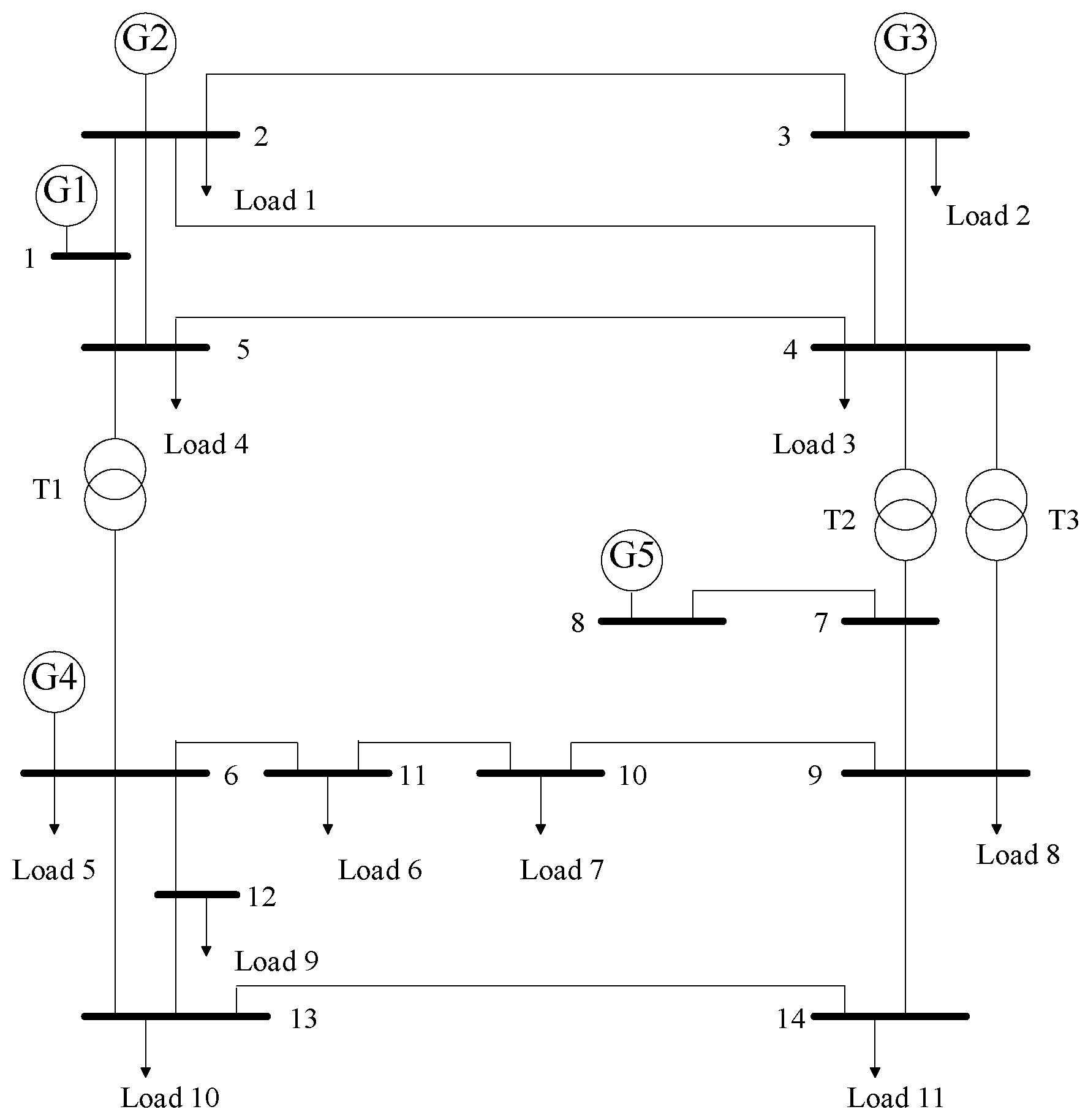
Figure 7.
The impact of tradeoff factor.

Figure 8.
The convergence of the temperature settings.

Figure 9.
The convergence of the power supply.

Figure 10.
The convergence of the retail price.

Figure 11.
The convergence of the temperature settings.
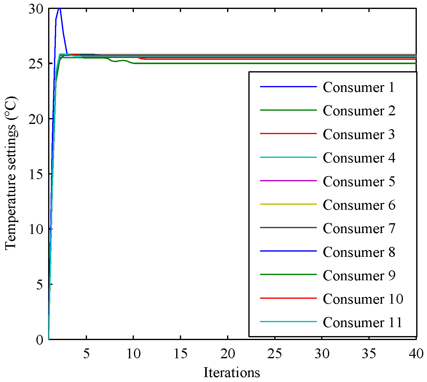
Figure 12.
The convergence of the power supply.
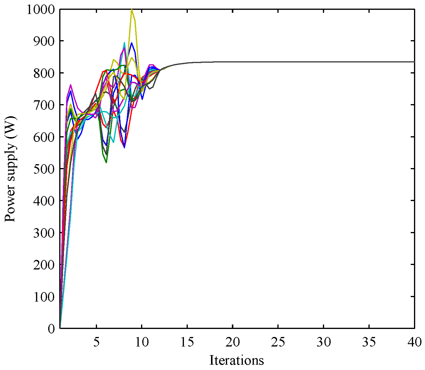
Figure 13.
The convergence of the retail price.
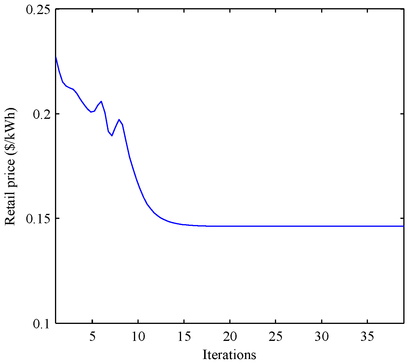
Figure 14.
The retail prices under different EEGs.
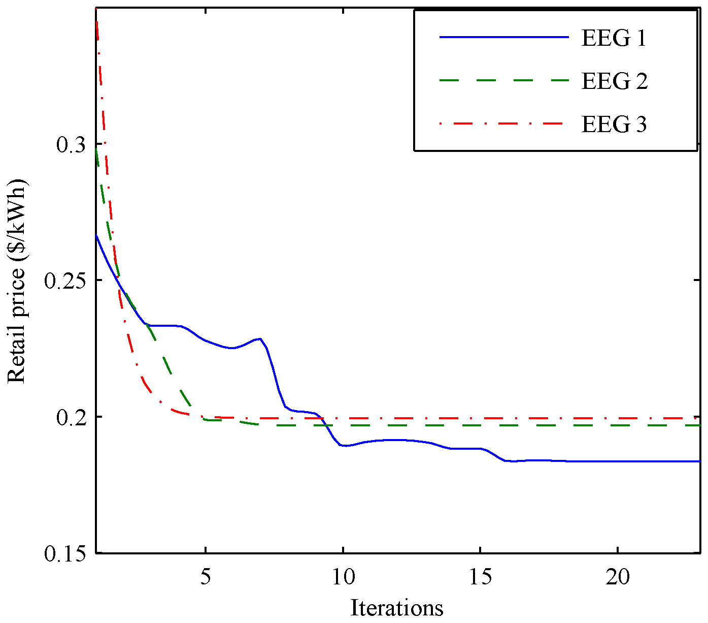
Figure 15.
The power supply under different EEGs.


Table 1.
The specific explanation of the parameters.
| Parameters | Explanation |
|---|---|
| M | Human body’s energy metabolic rate () |
| W | Human body’s mechanical work () |
| Pa | Vapour pressure around body (Pa) |
| Air temperature (°C) | |
| Area coefficient of clothing | |
| Ttemperature of clothes (°C) | |
| Indoor’s mean radiant temperature (°C) | |
| Convective heat transfer coefficient (W/(K)) | |
| Heat resistance of clothes ((K)/W) | |
| Air velocity (m/s) |
Table 2.
Parameter Settings.
| Parameters | Values |
|---|---|
| Outdoor temperature (°C) | |
| Transmission area () | |
| Heat transfer constant () | |
| Specific heat of air (°C) | |
| Air density () | |
| Wind speed coefficient | |
| Outdoor heat coefficient | |
| Effective infiltration area () | |
| Building height (m) | |
| Solar and internal load (W) |
Table 3.
The cost data.
| Discomfort Cost ($) | Generation Cost ($) | Total Costs ($) | |
|---|---|---|---|
| 0.1 | 8.1279 | 11.5264 | 19.6543 |
| 0.2 | 7.0753 | 11.6035 | 18.6788 |
| 0.3 | 6.7075 | 11.7344 | 18.4419 |
| 0.4 | 4.7092 | 12.5458 | 17.2550 |
| 0.5 | 5.0396 | 12.4054 | 17.4450 |
| 0.6 | 4.3398 | 12.8159 | 17.1557 |
| 0.7 | 3.3431 | 14.3050 | 17.6481 |
| 0.8 | 3.0488 | 15.4414 | 18.4902 |
| 0.9 | 3.0605 | 15.3121 | 18.3726 |
Table 4.
The temperature settings and energy consumption in IEEE 9-bus system.
| Consumer i | Temperature (°C) | Power Consumption (kW) |
|---|---|---|
| 1 | 25.4534 | 0.6986 |
| 2 | 25.0573 | 1.6701 |
| 3 | 24.5559 | 3.6015 |
| 1–3 | / | 5.9702 |
Table 5.
The power supply on each bus in IEEE 9-bus system.
| Buses i | Power Supply (W) |
|---|---|
| 1 | 663.3679 |
| 2 | 663.3646 |
| 3 | 663.3654 |
| 4 | 663.3676 |
| 5 | 663.3669 |
| 6 | 663.3692 |
| 7 | 663.3686 |
| 8 | 663.3693 |
| 9 | 663.3683 |
| 1–9 | 59702 |
Table 6.
The temperature settings and energy consumption in IEEE 14-bus system.
| Consumer i | Temperature (°C) | Power Consumption (kW) |
|---|---|---|
| 1 | 25.7925 | 0.3526 |
| 2 | 25.5883 | 0.6228 |
| 3 | 25.3969 | 0.9958 |
| 4 | 25.7143 | 0.7118 |
| 5 | 25.7578 | 0.7356 |
| 6 | 25.7708 | 0.7896 |
| 7 | 25.5143 | 1.2350 |
| 8 | 25.7187 | 1.0332 |
| 9 | 25.0050 | 2.2812 |
| 10 | 25.5317 | 1.5131 |
| 11 | 25.6491 | 1.4117 |
| 1–11 | / | 11.6825 |
Table 7.
The power supply on each bus in IEEE 14-bus system.
| Buses i | Power Supply (W) |
|---|---|
| 1 | 834.4625 |
| 2 | 834.4609 |
| 3 | 834.4616 |
| 4 | 834.4629 |
| 5 | 834.4693 |
| 6 | 834.4612 |
| 7 | 834.4625 |
| 8 | 834.4650 |
| 9 | 834.4621 |
| 10 | 834.4595 |
| 11 | 834.4648 |
| 12 | 834.4673 |
| 13 | 834.4591 |
| 14 | 834.4637 |
| 1–14 | 11682 |
© 2017 by the authors. Licensee MDPI, Basel, Switzerland. This article is an open access article distributed under the terms and conditions of the Creative Commons Attribution (CC BY) license (http://creativecommons.org/licenses/by/4.0/).
Share and Cite
MDPI and ACS Style
Ma, K.; Bai, Y.; Yang, J.; Yu, Y.; Yang, Q. Demand-Side Energy Management Based on Nonconvex Optimization in Smart Grid. Energies 2017, 10, 1538. https://doi.org/10.3390/en10101538
AMA Style
Ma K, Bai Y, Yang J, Yu Y, Yang Q. Demand-Side Energy Management Based on Nonconvex Optimization in Smart Grid. Energies. 2017; 10(10):1538. https://doi.org/10.3390/en10101538
Chicago/Turabian StyleMa, Kai, Yege Bai, Jie Yang, Yangqing Yu, and Qiuxia Yang. 2017. "Demand-Side Energy Management Based on Nonconvex Optimization in Smart Grid" Energies 10, no. 10: 1538. https://doi.org/10.3390/en10101538
Note that from the first issue of 2016, this journal uses article numbers instead of page numbers. See further details here.