1. Introduction
Complex fracture networks in shale oil reservoirs make the accurate modeling of oil production in these reservoirs very challenging. Three classes of models, equivalent continuum models (ECMs), dual-continuum models, and discrete fracture models (DFMs) are applied to model fractured systems.
Based on the equivalent continuum theory, Snow [
1] first proposed the ECM which describes flow in fractured media mathematically. Since the introduction of this model, several scholars have conducted research on this method, such as Oda [
2] and Tian [
3].
Dual-continuum modeling is the conventional method for simulating fractured reservoirs and is widely used in the industry. In the 1960s, Barenblatt et al. [
4] first established dual-porosity model to simulate matrix-fracture flow systems. Afterward, Warren and Root [
5] developed a more complete dual-porosity model. Kazemi et al. [
6] and Saidi [
7] developed dual-porosity simulators, which extended the Warren and Root approach to multiphase flow. Recently, Pruess and Narasimhan [
8] subdivided matrix rock gridding and proposed a multiple interacting continua (MINC) model in 1985. Furthermore, Moinfar et al. [
9] proved that the dual-continuum model could not provide accurate solutions in the high-localized anisotropy and presence of large-scale fractures in 2012.
The DFM method, in which an element and a control volume explicitly represents each fracture by, was established to model fluid flow in individual fractures and provide more realistic representations of fractured reservoirs than dual-continuum models. Most DFMs honor the geometry and the location of fracture networks with relying on unstructured grids. Kim and Deo [
10] adopted a finite element method to perform discretization for DFM and to combine matrix and fractures based on the superposition principle. Later, Karimi-Fard and Firoozabadi [
11] applied DFM to solve the two-phase flow problem in the fractured media. Likewise, Monteagudo and Firoozabadi [
12] and Matthäi and Belayneh [
13] used control-volume finite element methods for multiphase flow in fractured media and developed numerical simulators. Karimi-Fard et al. [
14] extended DFMs compatible with multiphase reservoir simulators based on an unstructured control-volume finite difference formulation. In addition, Li and Lee [
15] and Moinfar et al. [
9] developed embedded discrete fracture models (EDFMs), which use a structured grid to represent the matrix and introduce additional fracture control volumes by computing the intersection of fractures with the matrix grid. Recently, more attention is paid to the EDFM because of its flexibility and accuracy. Hadi Hajibeygi et al. [
16] proposed the iterative multiscale finite volume (i-MSFV) approach to improve the efficiency and the accuracy for fractured porous media, and the results are very promising. Ţene et al. [
17] proposed a projection-based EDFM to deal with cases where the fracture permeability lies below that of the matrix. The fracture-crossflow-equilibrium method was proposed in 2017 by Ali Zidane and Abbas Firoozabadi [
18] to study compositional two-phase flow in the fractured media; simulation results showed that central processing unit (CPU) time with fractured media and without fractured media differs by less than a factor of two. Sander Pluimers [
19] introduced hierarchical fracture modeling (HFM) in 2015, upscaling small- and medium-scale fractures into an effective matrix permeability and studying upscaling criteria for the HFM.
In order to balance accuracy, computational efficiency, and field practice, we propose a new method that integrates EDFM and dual-porosity, dual-permeability (DPDP) concepts to model the production process in shale oil reservoirs. The developed method could explicitly describe large-scale permeable fractures as flow conduits and simulate natural fracture networks that connect the global flow in stimulated areas of shale oil reservoirs. It may take years to reach the pseudo-steady state in the matrix systems, so the traditional dual-porosity approach can result in large inaccuracies. With the newly developed simulator, we perform comprehensive simulation studies to determine the key factors of fractures and reservoir which affect the ultimate oil recovery in shale oil reservoirs. Different engineering factors and injection strategies are also analyzed and compared to provide guidance for production optimization during the CO2 huff-and-puff process.
2. Methodology
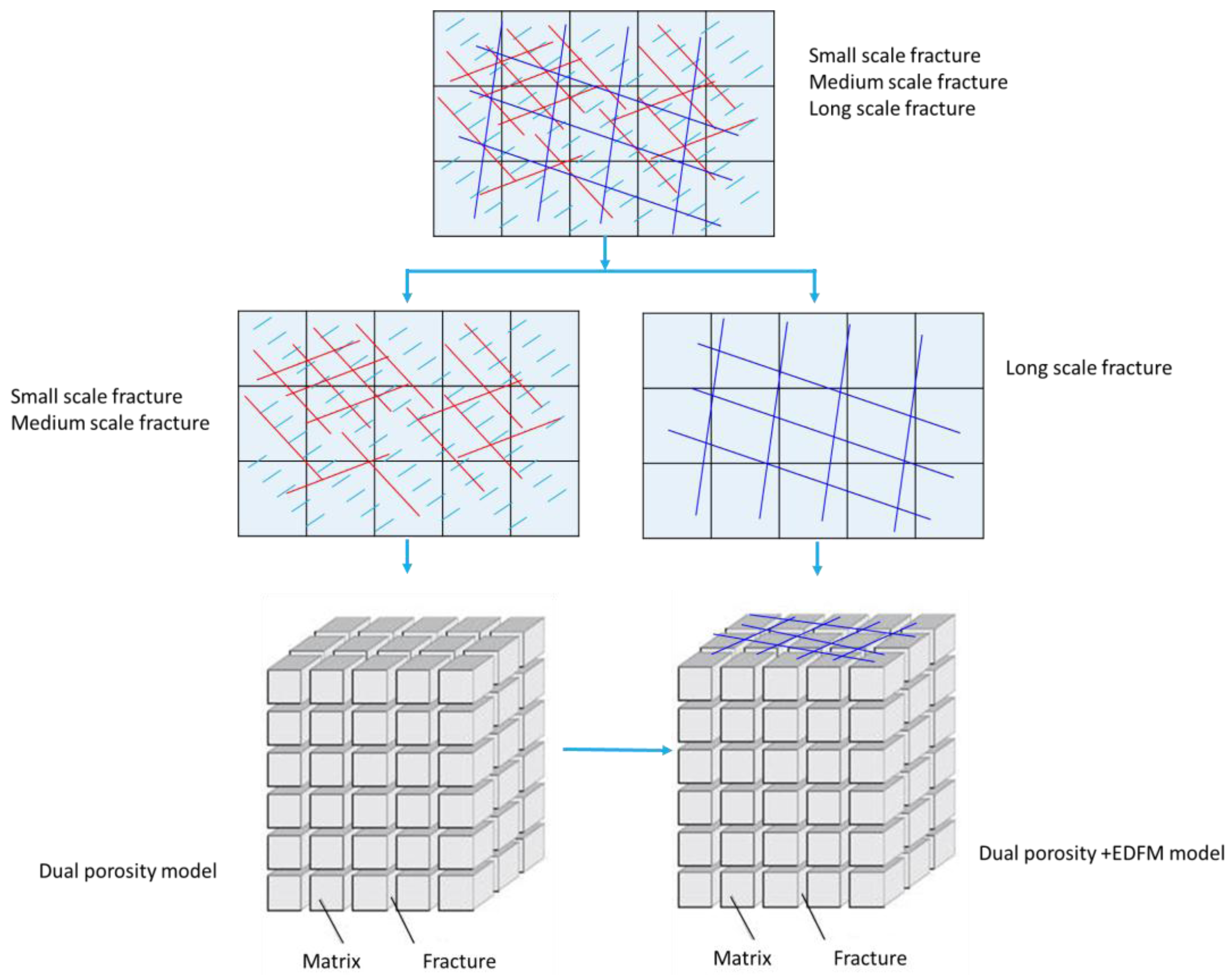
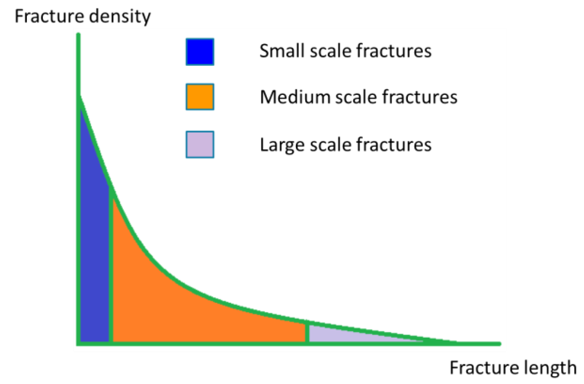
Naturally fractured reservoirs typically have a wide range of fracture length-scales, ranging from micrometers up to several hundred meters.
Figure 1 shows the correlation between fracture density and length. The small- to medium-scale fractures usually have higher densities than large-scale fractures in the reservoir. These fractured reservoirs are geologically too complex to be fully represented by a DFM because it individually represents each fracture.
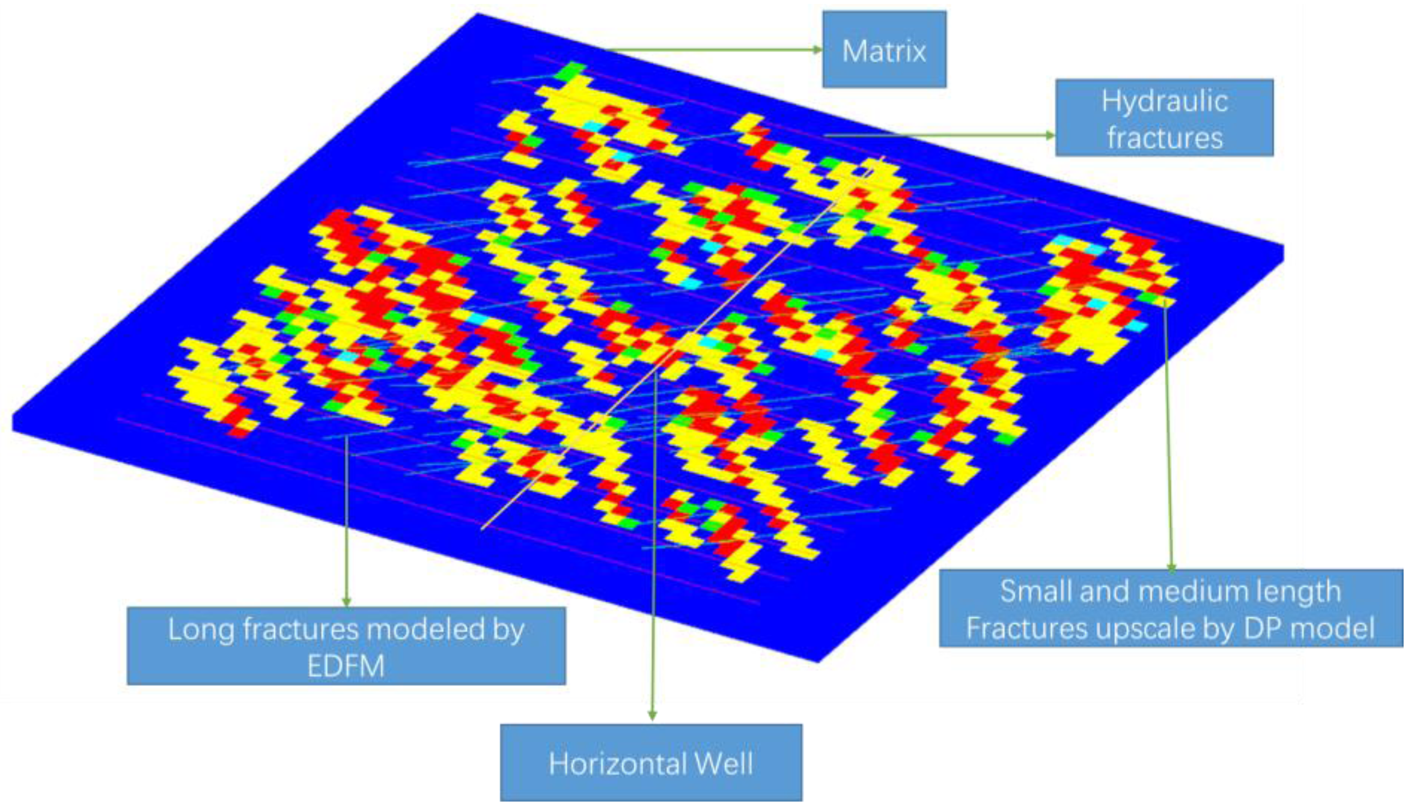
Therefore, a new model is developed combining the EDFM with the DPDP model to obtain a simplified reservoir model. As shown in
Figure 2, large-scale fractures are assumed to be main fluid conduits and to have a big impact on flow pattern. For this reason, large-scale fractures are kept explicitly in the EDFM to model them with great accuracy. Medium-scale fracture lengths are about one to five times of the grid size and are modeled by the dual-porosity model. Small-scale fractures are expected to have a small impact on flow field. These fractures are approximated by effective “damaged matrix rock” properties, which are obtained by upscaling methods. This way, the small and medium fractures are deducted from the EDFM, resulting in a big reduction in the simulation effort.
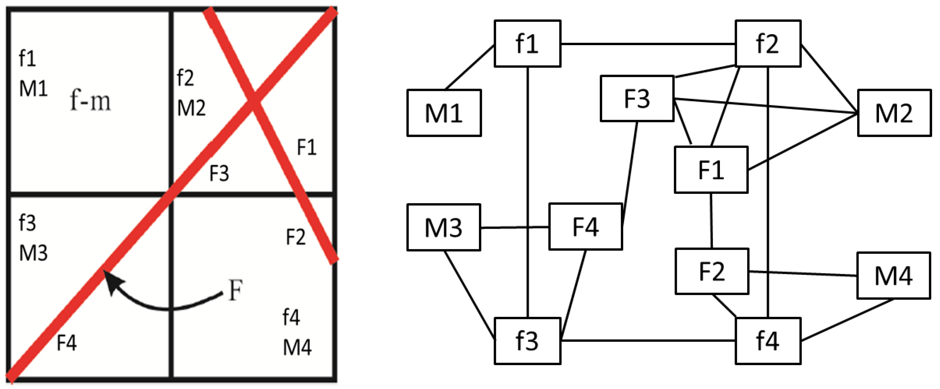
The key aspect of the new model is the calculation of connection transmissibility for flux interaction among different continua. Non-neighboring connections (NNCs) are subsequently determined as adding cells to represent fracture segments.
Figure 3 illustrates the connection list of continua in the computational domain for a simple scenario. We adopted and extended the definition of NNCs, Four types of NNCs, which were adopted and extended from Moinfar [
20], are defined as follows:
NNC type I: connection between a fracture segment and the fracture cell in the dual-porosity model;
NNC type II: connection between fracture segments in an individual fracture;
NNC type III: connection between intersecting fracture segments;
NNC type IV: connection between a fracture segment and the matrix cell in the dual-porosity model.
2.1. NNC Type I: Connection between a Fracture Segment and the Fracture Cell in the Dual-Porosity Model
The NNC transmissibility factor between the fracture segment and fracture cell in the dual-porosity model depends on the fracture geometry and fracture permeability. As a fracture segment fully penetrates a matrix cell, the fracture-fracture cell transmissibility factor is:
where
is the area of the fracture segment on one side and
is the permeability tensor, which is calculated as:
is the embedded fracture permeability tensor,
is the fracture cell permeability tensor, and
is the average normal distance from fracture to embedded fracture, which is calculated as:
where
V is the volume of the fracture cell,
dV is the volume element of matrix, and
is the distance from the volume element to the fracture plane.
2.2. NNC Type II: Connection between Fracture Segments in an Individual Fracture
The transmissibility factor between a pair of neighboring segments 1 and 2 is calculated using a two-point flux approximation scheme as:
where
and
are the fracture permeability,
is the area of the common face for these two segments, and
and
are the distances from the centroids of segments 1 and 2 to the common face, respectively.
2.3. NNC Type III: Connection between Intersecting Fracture Segments
It is very challenging to model fracture intersection accurately and efficiently for DFM due to the complexity of flow behavior at the fracture intersection. In 2014, Moinfar et al. [
9] simplified this problem. They approximated the mass transfer at the fracture intersection by assigning a transmissibility factor between intersecting fracture segments. The transmissibility factor is given as:
where
Lint is the length of the intersection line and
and
are the weighted average of the normal distances from the centroids of the subsegments (on both sides) to the intersection line.
2.4. NNC Type IV: Connection between a Fracture Segment and the Matrix Cell in the Dual-Porosity Model
The matrix permeability and fracture geometry determine the NNC transmissibility factor between matrix and fracture segment. When a matrix cell is fully penetrated by a fracture segment, the matrix-fracture transmissibility factor is:
where
is the area of the fracture segment on one side and
is the permeability tensor, which is calculated as:
is the fracture permeability tensor,
is the matrix permeability tensor, and
is the average normal distance from matrix to fracture, which is calculated as:
where
V is the volume of the matrix cell,
dV is the volume element of matrix, and
is the distance from the volume element to the fracture plane.
If the fracture does not fully penetrate the matrix cell, the pressure distribution in the matrix cell may deviate from previous assumptions. As a result, the calculation of the transmissibility factor is complex. To make the method non-intrusive, it was assumed the transmissibility factor is proportional to the area of the fracture segment inside of the matrix cell.
3. Model Validation
As mentioned by Ţene et al. [
17], using EDFM for fractures with very low permeability may create inaccurate results. So only permeable fractures are considered in this study. In this section, we present a three-dimensional (3D) case with two sets of permeable fractures. The hybrid EDFM-DPDP approach is compared to EDFM, DFM, and dual-porosity approaches to verify the accuracy of the hybrid EDFM-DPDP method in modeling fracture networks.
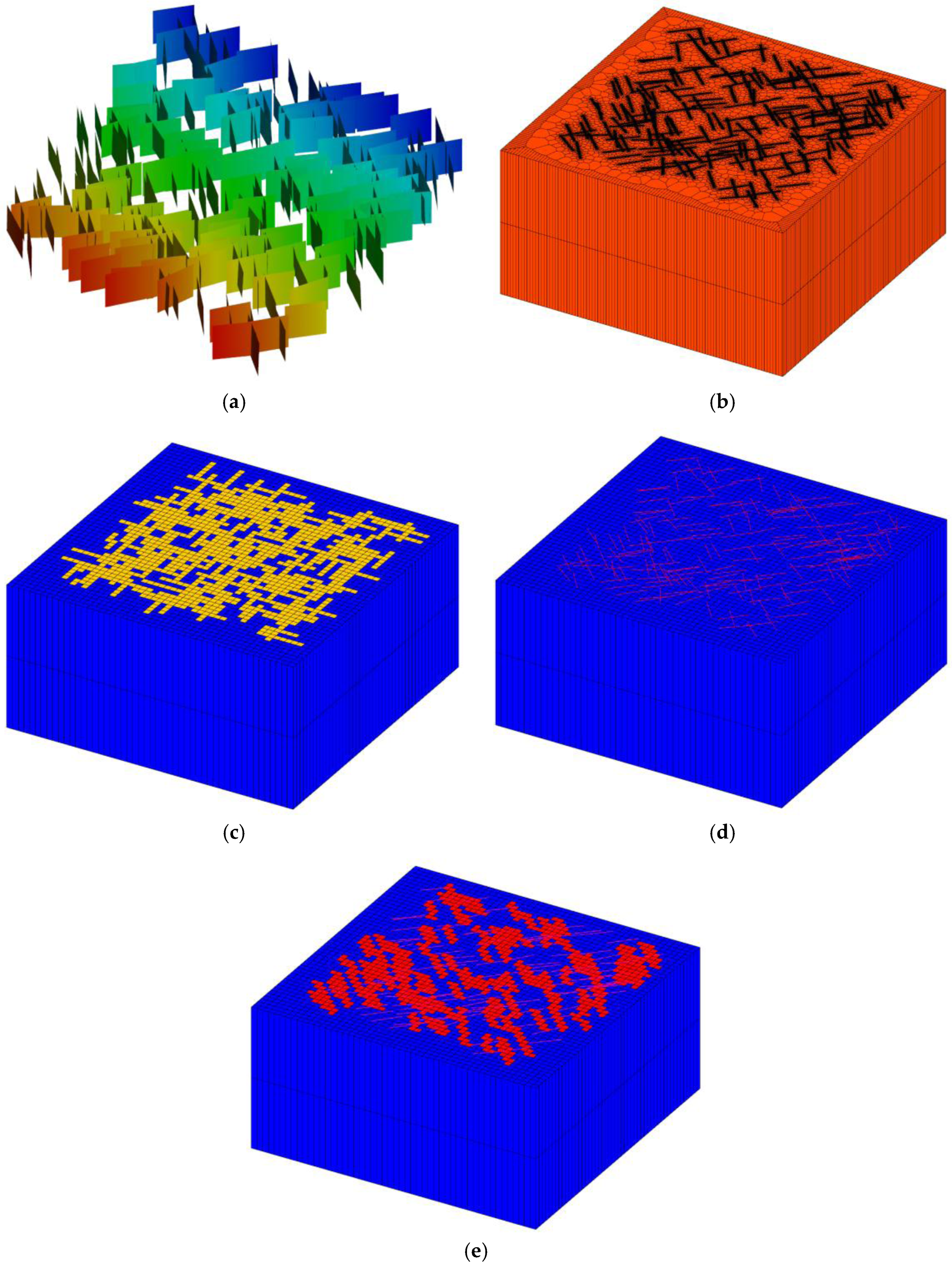
Figure 4 shows the dimensions of the reservoir and the positions of fracture planes.
Figure 4a shows the fracture system used in this study.
Figure 4b is the DFM with 213,810 cells.
Figure 4c is the DPDP model, with a flow-based method used to homogenize all of the fractures in the upscaling process.
Figure 4d is the EDFM, explicitly showing the fractures.
Figure 4e shows the hybrid EDFM-DPDP method, picturing one set of fractures by dual porosity and the other set of fractures by EDFM. In the hybrid EDFM-DPDP method, small- and medium-scale fractures are upscaled by a flow-based method.
The reservoir dimensions are 1000 × 1000 × 20 ft. The fractures fully penetrate the reservoir vertically (with a height of 20 ft from the top to the bottom of the reservoir). The width and permeability of the fractures is 0.01 ft and 500 md, respectively. As a result, the fracture conductivity is 5 md-ft. A uniform 50 × 50 × 2 matrix grid is defined in dual-porosity, EDFM, and hybrid EDFM-DPDP methods. The dimensions of the matrix cells are 20 × 20 × 10 ft. Five vertical wells are defined in the reservoir: one is a water injector located at the reservoir center, with an injection rate of 200 stb/day and limited bottomhole pressure (BHP) no more than 5000 psi; the other four wells are oil producers located at the corner, with oil rates of 50 stb/day and limited BHP no less than 500 psi.
This example is for water injection of a low-permeability oil reservoir. The reservoir is isotropic as the permeabilities in the X, Y, and Z directions are the same. The Corey model was used for the relative permeability curve for both matrix and fracture. Peaceman’s model was applied to calculate the well indices. The detailed reservoir and fluid properties are summarized in
Table 1.
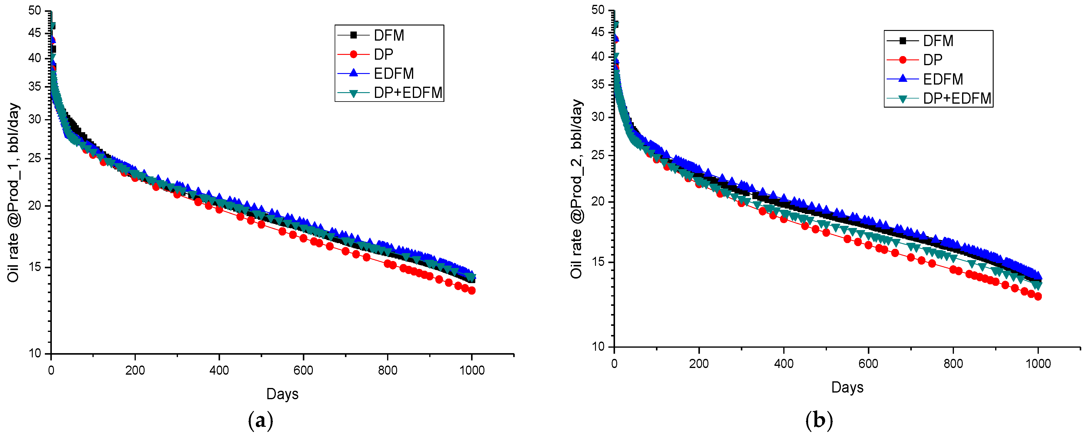
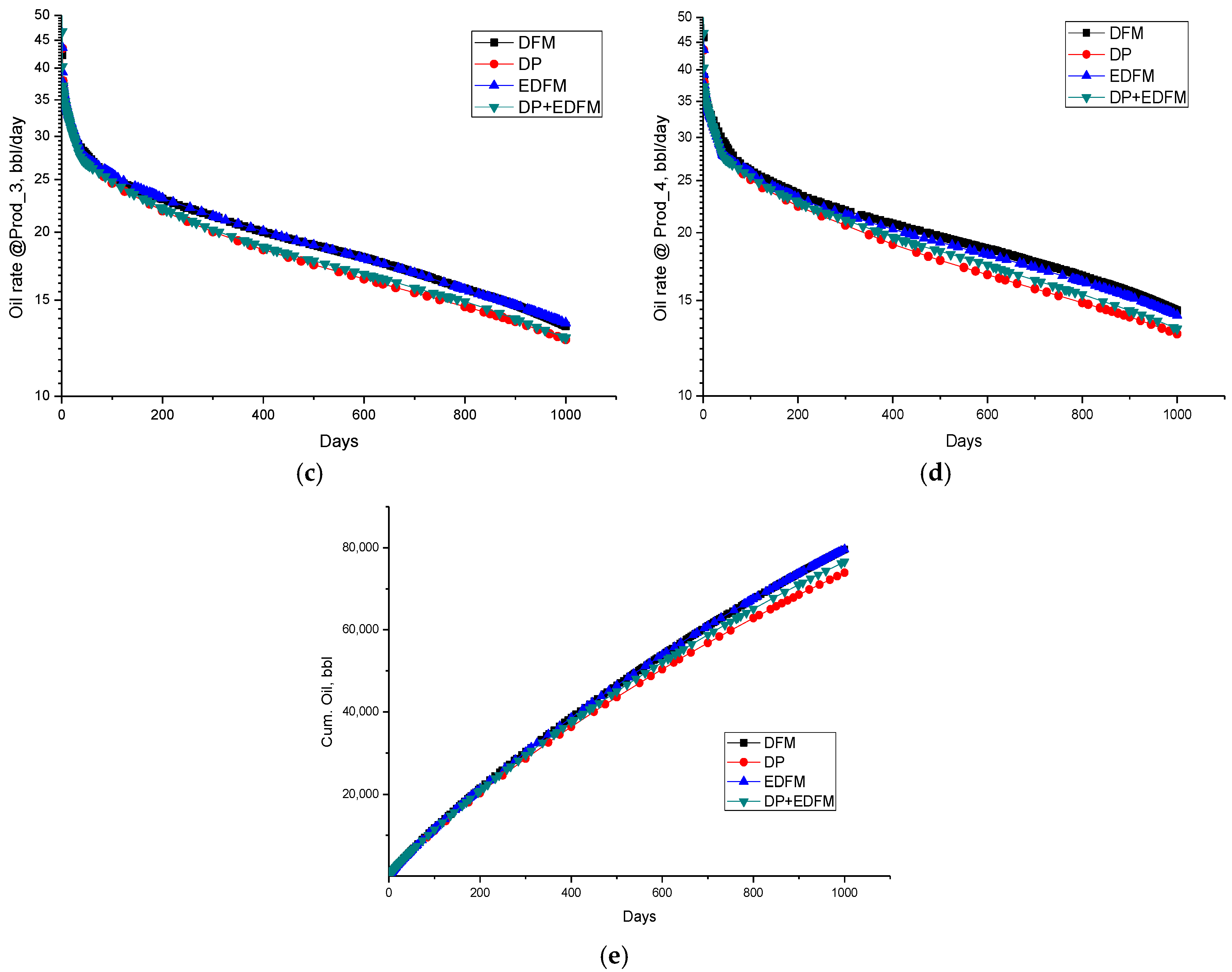
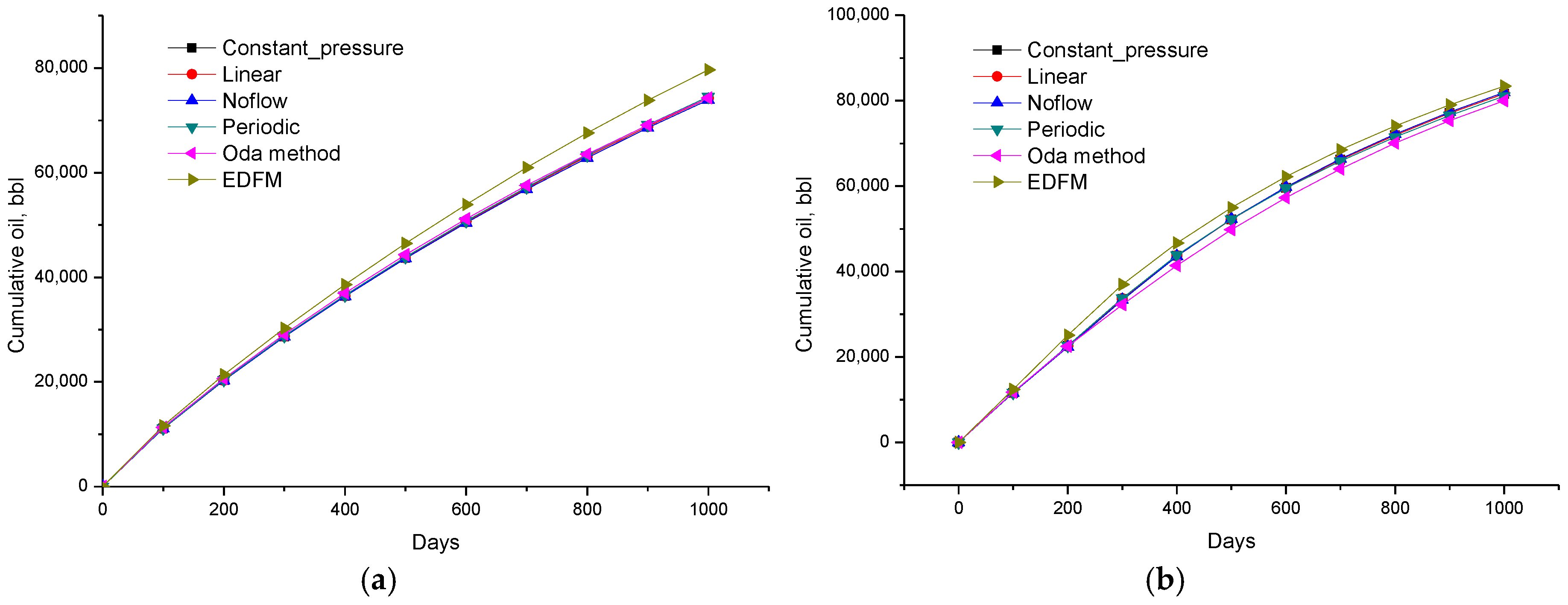
Figure 5 shows the well oil production rates and the cumulative oil production of different models. The results of EDFM and DFM are highly consistent in these plots, and the dual-porosity model is significantly different among these methods, while curves from the hybrid EDFM-DPDP method are between that from dual-porosity and DFM methods, indicating that EDFM improves the accuracy and verifying of the the EDFM. The upscaling method and grid refinement are considered as other ways to improve accuracy of the dual-porosity model. In this study, we also run five cases with different upscaling methods (Oda method and flow-based method with different boundaries: linear, constant pressure, no-flow, and periodic) and three cases with different grid sizes from 5 to 20 for dual porosity. The comparison among different upscaling methods with the EDFM method is shown in
Figure 6.
Figure 6a indicates that different upscaling methods reach similar results for water flooding, and
Figure 6b shows the difference between the Oda method and other upscaling methods for gas flooding. Meanwhile, the figure also shows a significant difference between these upscaling methods and EDFM.
Capillary pressure plays an important role in fractured reservoir. In this study, different methods with capillary pressure for water flooding are studied. As shown in
Figure 7, the difference between EDFM and DP methods is about 3.5–4.0%. While the difference is 1.5% between EDFM and hybrid EDFM and DP methods.
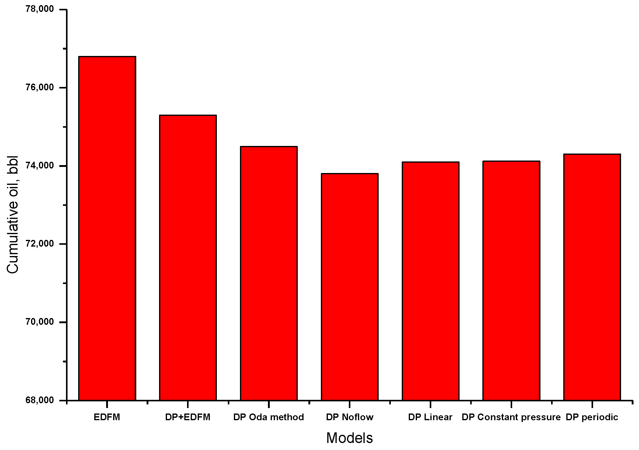
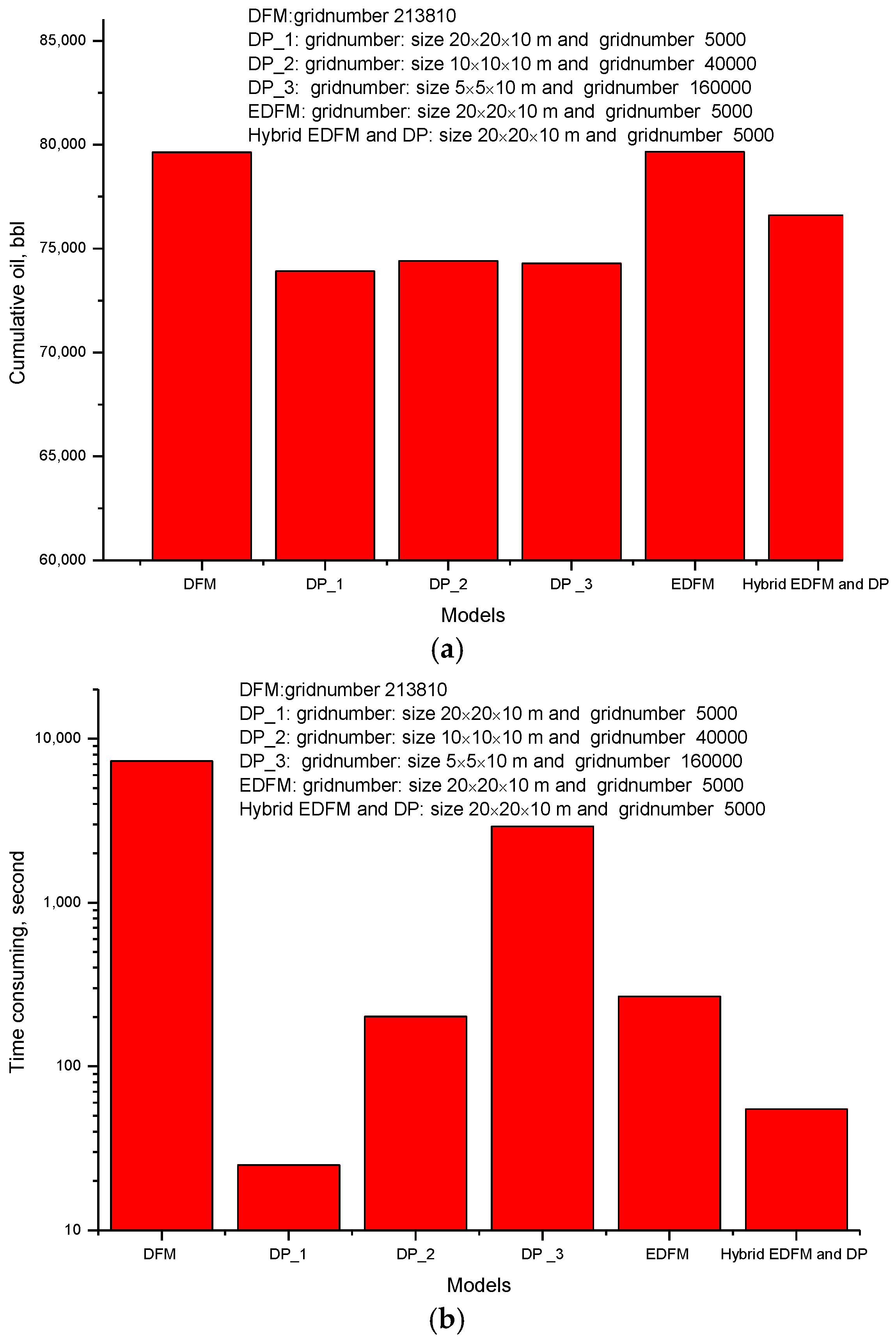
Figure 8 shows the cumulative oil and time consumption vs. different models. We can find that the refinement grid from 20 to 5 m for the dual-porosity model doesn’t improve accuracy in this study, and time consumption increases from 25 to 2927 s when grid number increases from 5000 to 16,000 in the DP models. The figure also points out that DFM consumes 4322 s, EDFM takes 268 seconds, and the hybrid EDFM-DPDP method takes 55 s. All of the simulations were performed on a 2.6 GHz, Intel CoreDuo CPU. The time consumption of the hybrid EDFM-DPDP method is only 1/80 that of the DFM method and 1/5 that of the EDFM method. From the study, we conclude that EDFM maintains accuracy and saves CPU time.
4. Comprehensive Sensitivity Studies
There is high uncertainty in shale oil formations because of many uncertain parameters, such as reservoir permeability, fracture half-length, number of fractures, and fracture conductivity. In addition, parameters related to CO2 huff-and-puff are also uncertain, such as CO2 injection rate, injection time, and soaking time, and the number of cycles of CO2 huff-and-puff. Accordingly, in the subsequent simulation study, we perform a series of simulations to investigate the impacts of these uncertain parameters related to the CO2 huff-and-puff process.
4.1. Reservoir Model
As shown in
Figure 9, a base model is constructed to perform simulation studies for a single horizontal well with natural fractures and multiple hydraulic fractures in a shale oil reservoir. Several reservoir and fracture parameters are analyzed, including natural fracture permeability, hydraulic fracture permeability, hydraulic fracture half-length, hydraulic fracture stages, and so on.
The parameters assumed for the model are summarized in
Table 2. The properties of the components used for the simulation studies are shown in
Table 3.
In huff-and-puff recovery, we maintain injection pressure to be higher than the minimum miscibility pressure. In this study, the minimum miscibility pressure is estimated to be 3000 psi based on experiment and slim-tube simulation. Therefore, well BHP is set to 4000 psi during production and well BHP is set to 6000 psi during the CO
2 injection. During the injection process, pure CO
2 is injected into the reservoir. Specifically, the well pressure is fixed at 4000 psi from day 1 to 300 to carry out primary recovery. Then, the well is operated as an injection well from day 301 to 360 at a fixed pressure of 4000 psi. During this period, pure CO
2 is injected into the reservoir. From day 361 to 390, the well is closed, letting the CO
2 mix with oil in the reservoir. From day 391 to 480, the well is reopened to produce hydrocarbons at a fixed pressure of 4000 psi. The same CO
2 huff-and-puff steps are repeated until day 1200, giving rise to five cycles of CO
2 huff-and-puff. Detailed steps are listed in
Table 4.
4.2. Large Natural Fracture Permeability
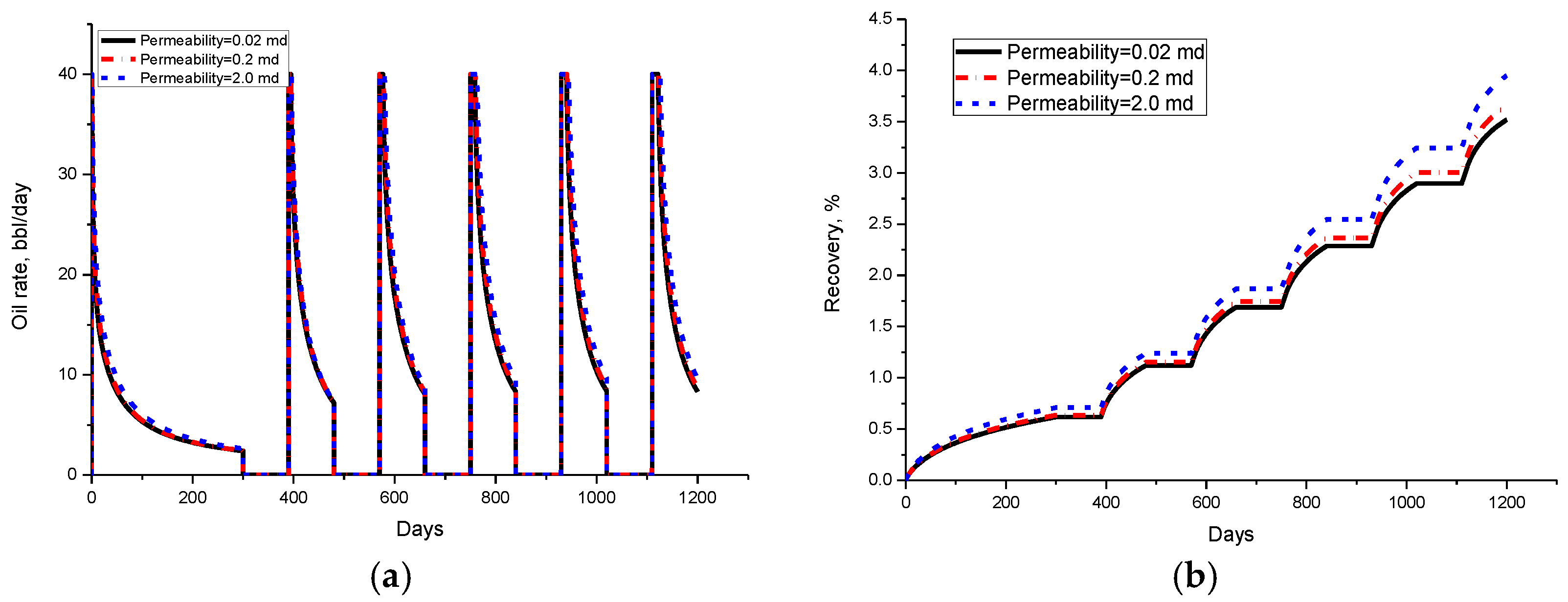
A sensitivity study was conducted on large natural fracture permeability for 0.02, 0.2, and 2 md with 16 hydraulic fractures.
Figure 10a shows that the oil rate depletes from 40 to 2.4 m
3/day for the first 300 days, with primary recovery being only 0.62%. After 60 days of gas injection and 10 days of soaking, oil rate increases to 40 m
3/day and decreases to 7 m
3/day at the end of the first cycle.
Figure 10b shows the oil recovery increase from 3.51 to 3.95% when natural fracture permeability increases from 0.02 to 2.0 md, which means a 12.5% improvement. The results illustrate that using gas huff-and-puff could significantly improve production and remarkably impact the permeability of the cumulative oil production. Higher natural fracture permeability can provide higher flow conductivity and result in higher oil recovery.
4.3. Hydraulic Fracture Permeability, Length, and Stages
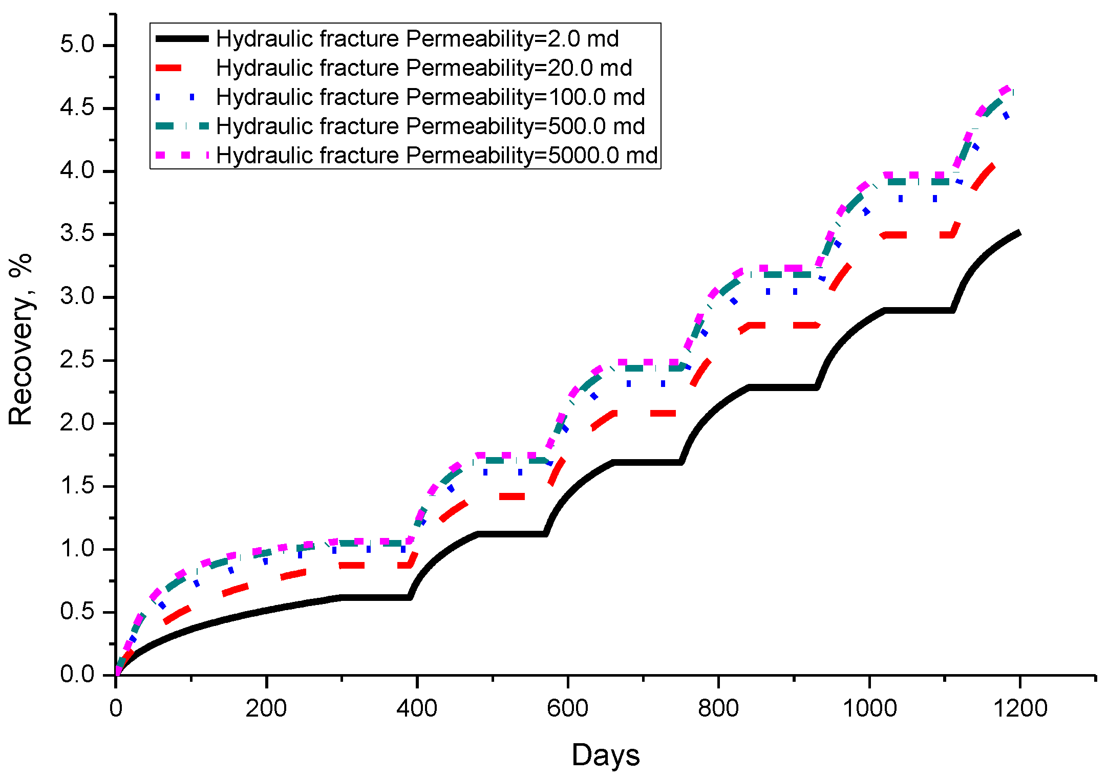
A simulation study is performed on hydraulic fracture permeability for 2, 20, 100, 500, and 5000 md, with natural fracture permeability of 0.02 md, number of hydraulic stages of 16, and a half-length of 400 ft.
Figure 11 shows the simulation results of five different hydraulic fracture permeabilities. The Figure illustrates that a higher hydraulic fracture permeability results in a higher recovery. Oil recovery increases from 3.51 to 4.51% when hydraulic fracture permeability increases from 2 to 100 md. However, oil recovery only increases 0.20% when permeability increases from 100 to 5000 md. The results illustrate that there exists an optimum value of hydraulic fracture permeability. Over the optimum value (100 md in this case), increasing hydraulic fracture permeability has a slight impact on oil recovery.
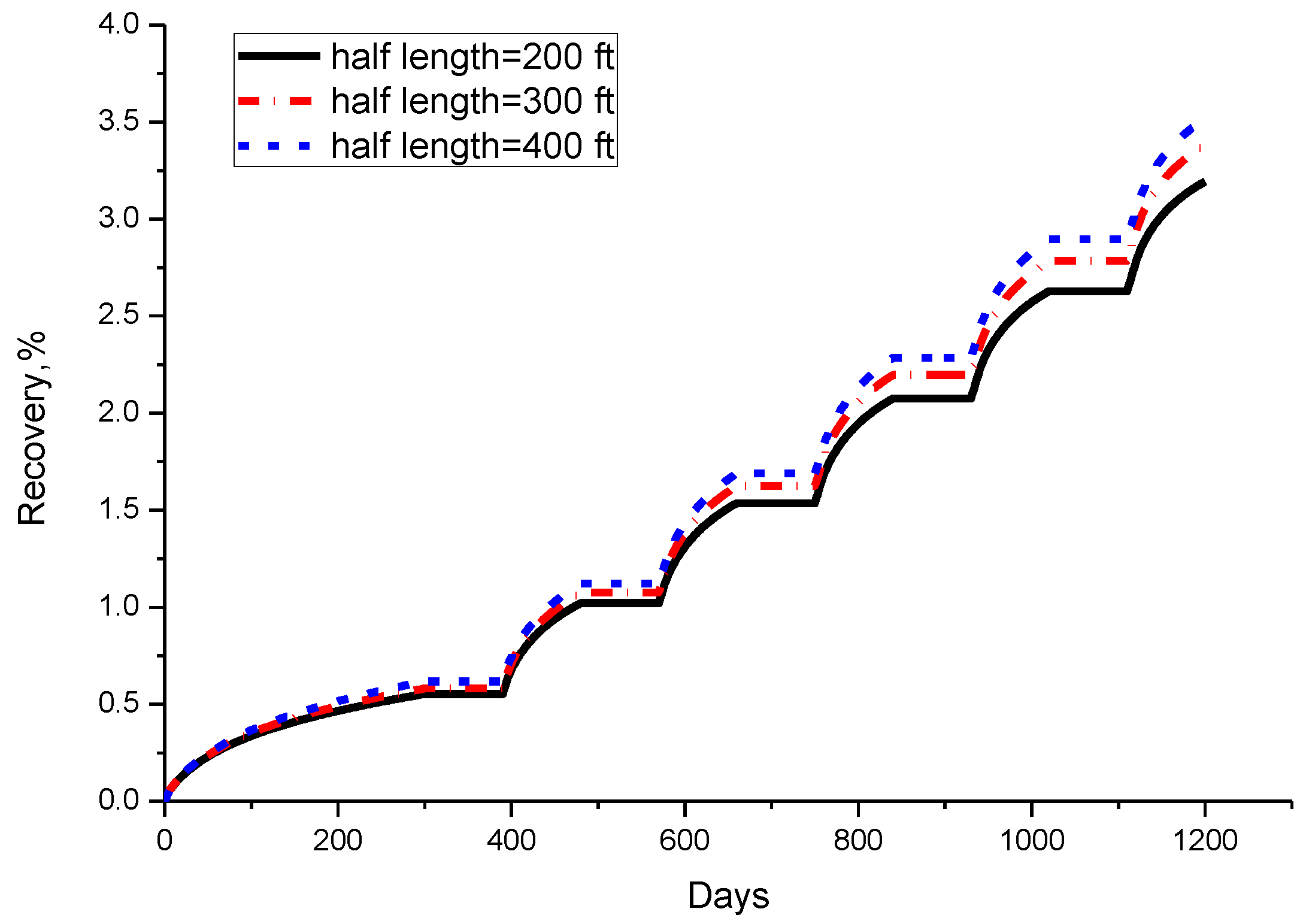
A comparison of oil recovery factor with different hydraulic fracture lengths is shown in
Figure 12. In this study, half-hydraulic-fracture-lengths for three cases are 200, 300, and 400 m. In the Figure, we can find that more oil can be produced with a longer hydraulic fracture. This is because longer hydraulic fractures yield more connections with natural fractures and matrix, resulting in higher oil recovery.
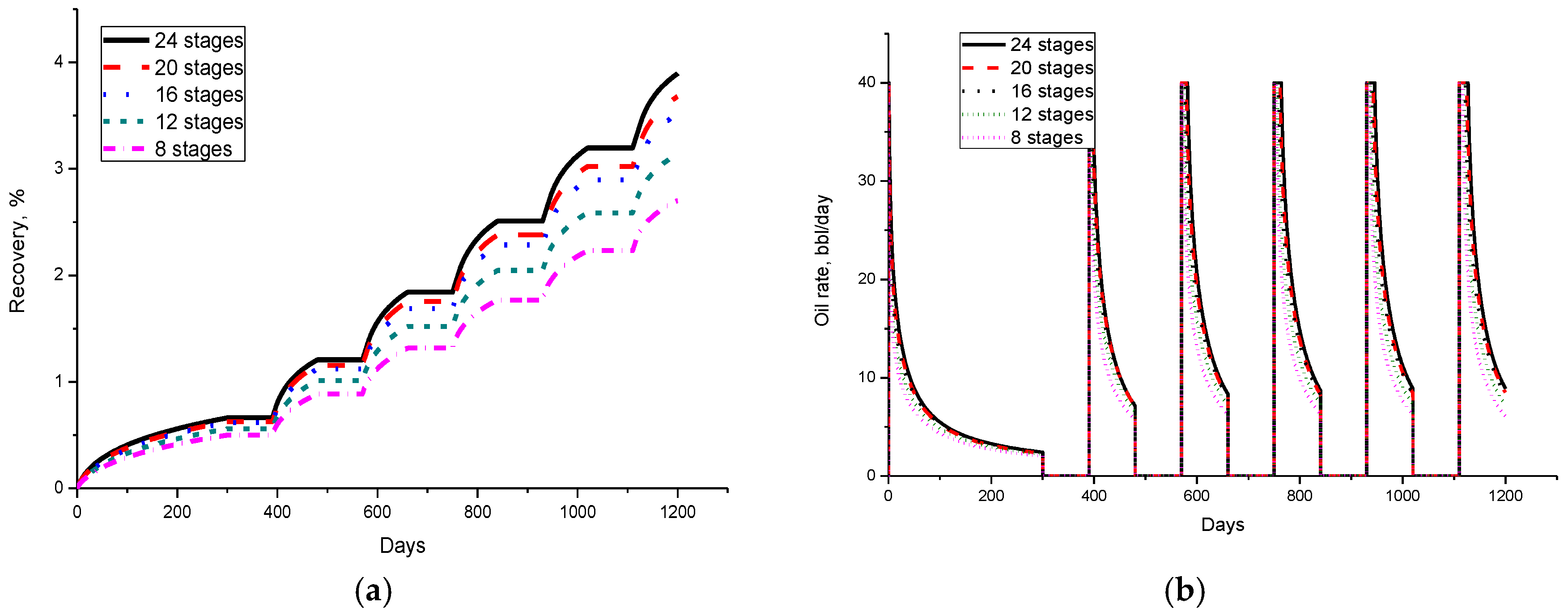
The hydraulic fracture stage is one important parameter with a significant impact on the CO
2 huff-and-puff process in shale oil. In this case, we run five cases with different numbers of stages from 8 to 24.
Figure 13 shows the recovery and oil rate vs. time at different fracture stages. When the stage increases from 8 to 24, oil recovery increases from 2.70 to 3.90%, which means recovery improved by 44% for the case at stage number 8.
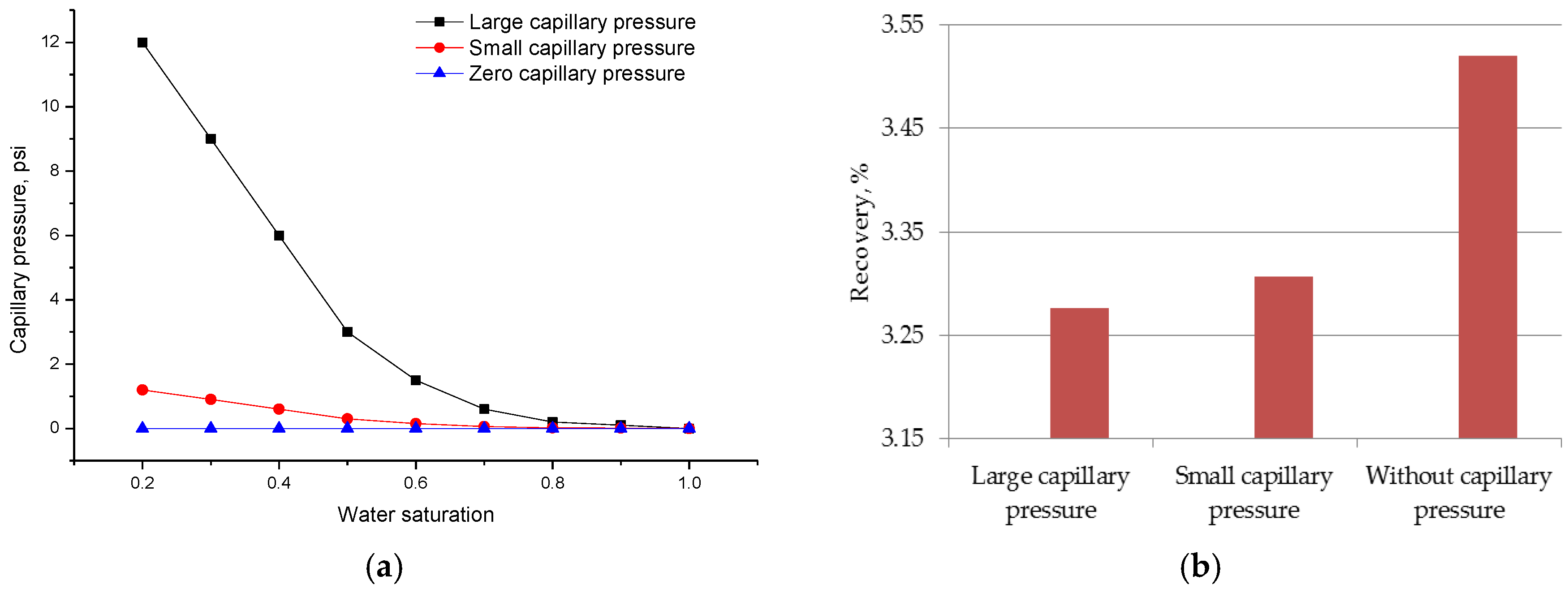
4.4. Capillary Pressure
Capillary pressure is one of the important parameters for fractured reservoir, especially when water flooding and gas flooding processes are involved. In this study, we run three cases with different capillary pressure curves.
Figure 14a shows capillary pressure curves used in the study and
Figure 14b shows the recovery for different curves. Recovery decreases with capillary pressure increases, and the case without capillary pressure reach higher recovery.
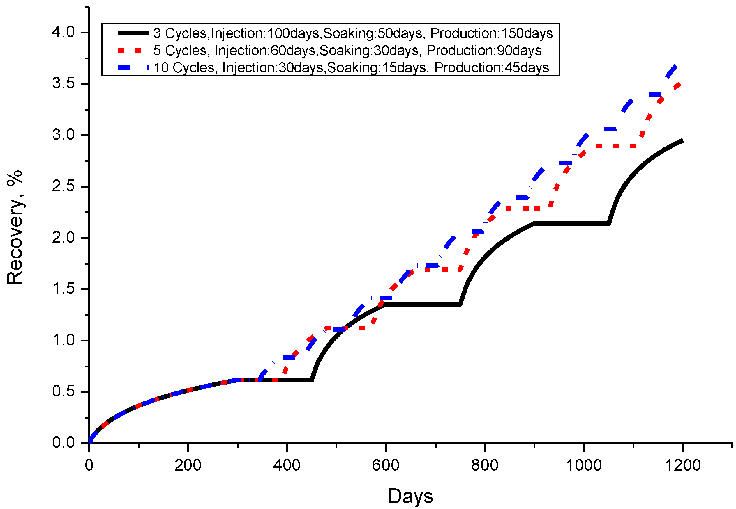
4.5. Huff-And-Puff Scenario
In order to investigate the effect of the huff-and-puff scenario on the CO
2 estimated oil recovery (EOR) process, several parameters are modified from the base model set up previously (the others remain unchanged). We compare three cases to determine the better injection strategy for the huff-and-puff scenario. The huff-and-puff patterns are summarized in
Table 5. We fix the total production and injection periods with different combinations.
Figure 15 shows the impact of different strategies on cumulative oil production. The Figure also shows that a reduced cycle length and increased cycles could increase the oil production.


