Article

Correlation Feature Selection and Mutual Information Theory Based Quantitative Research on Meteorological Impact Factors of Module Temperature for Solar Photovoltaic Systems

1
State Key Laboratory of Alternate Electrical Power System with Renewable Energy Sources, North China Electric Power University, Baoding 071003, Hebei, China
2
Department of Electrical and Computer Engineering, University of Illinois at Urbana-Champaign, Urbana, IL 61801, USA
3
Renewable Energy Department, China Electric Power Research Institute, Beijing 100192, China
4
Fenner School of Environment and Society, The Australian National University, Canberra, ACT 2601, Australia
*
Author to whom correspondence should be addressed.
Energies 2017, 10(1), 7; https://doi.org/10.3390/en10010007
Submission received: 2 September 2016 / Revised: 10 December 2016 / Accepted: 15 December 2016 / Published: 22 December 2016
(This article belongs to the Special Issue Innovative Methods for Smart Grids Planning and Management)

Abstract

:
The module temperature is the most important parameter influencing the output power of solar photovoltaic (PV) systems, aside from solar irradiance. In this paper, we focus on the interdisciplinary research that combines the correlation analysis, mutual information (MI) and heat transfer theory, which aims to figure out the correlative relations between different meteorological impact factors (MIFs) and PV module temperature from both quality and quantitative aspects. The identification and confirmation of primary MIFs of PV module temperature are investigated as the first step of this research from the perspective of physical meaning and mathematical analysis about electrical performance and thermal characteristic of PV modules based on PV effect and heat transfer theory. Furthermore, the quantitative description of the MIFs influence on PV module temperature is mathematically formulated as several indexes using correlation-based feature selection (CFS) and MI theory to explore the specific impact degrees under four different typical weather statuses named general weather classes (GWCs). Case studies for the proposed methods were conducted using actual measurement data of a 500 kW grid-connected solar PV plant in China. The results not only verified the knowledge about the main MIFs of PV module temperatures, more importantly, but also provide the specific ratio of quantitative impact degrees of these three MIFs respectively through CFS and MI based measures under four different GWCs.

1. Introduction

Given the increasingly serious problems of fossil energy shortage and greenhouse gas emissions, the need for sustainable and low-carbon energy technologies is on the rise [1]. As one of the most promising emerging renewable energy technologies, solar photovoltaic (PV) power generation has developed faster than anticipated [2]. The global installed PV capacity has grown from 0.96 GW in 1998 to 227 GW in 2015 [3]. There is no doubt that PV industry will play a more significant role in the future energy production. In particular, China has become the leader in the PV module manufacturing since 2009. At the end of 2013, China accounted for 67% of the total PV production [4]. According to the International Energy Agency (IEA), China leads the world in cumulative installed PV capacity, with over 110 GW by 2015, and solar power could potentially provide one-third of the global energy demand after 2060 [5,6].
However, there are still several problems that need to be solved due to the inherent properties of solar energy, such as its variability and uncertainty, particularly the sharp ramps under specific meteorological events and different outputs under variable weather conditions [7]. In order to maintain a consistent balance of supply and demand, power system operation is generally based on an understanding of the random variations in the load and the controllable and dispatchable conventional stand-by power generation plants [8]. Therefore, the predictability of the solar PV power generation and its accuracy are very important, both for the transmission and distribution sides. For the transmission side, non-dispatchable central large-scale solar PV plants with tempestuous and fast variable output may cause great issues to the active power balance and economic operation of regional grids. From the distribution side, roof-top PV, building integrated photovoltaic (BIPV) and other small-scale PV systems can be equivalent to negative electricity demand during the daytime with solar irradiance, which significantly reshape the traditional load curves by providing electricity directly to the load behind the meter. This effect will result in difficulties in load forecasting under different weather conditions, on which the dispatch operation depends [9]. Numerical weather prediction (NWP)-based multiple temporal and spatial scales solar PV power forecasting is a good measure to facilitate more economic decisions for the dispatch operation of power system. With this knowledge, the solar PV generation can be added into the grid operation more precisely like the economic dispatch considering the uncertainty of deep penetration of wind power, which will make it possible to schedule and adjust the dispatchable generators’ output to coordinate the fluctuation of solar PV plants as well as the wind farms and the electricity load from users’ demand [10].
In addition to the material of PV modules, the output power produced by PV modules (P) mainly depends on the amount of surface solar radiance flux on module plane (GT) and the PV cell temperature (Tc) [11], which can be approximately analyzed using Equation (1) [6]:
P = η r S G T [ 1 β ( T c T 0 ) + γ log G T ]
where P is PV power output, ηr is the reference module efficiency, S is the aperture surface area of PV module, β is temperature coefficients of PV modules, γ is solar irradiance coefficient of PV modules, Tc and T0 are PV cell temperature and reference values of temperature respectively, and finally, GT is surface solar radiance flux on module plane.
The γ, solar irradiance coefficient of PV modules, usually can be neglected because of its small value. Then Equation (1) is rewritten as Equation (2):
P = η r S G T [ 1 β ( T c T 0 ) ]
Reference [12] indicates that the temperature is almost uniform on the panel. Thus, an average PV module temperature (Tm) is used to replace the PV cell temperature. Therefore, Equation (2) can be rewritten as Equation (3):
P = η r S G T [ 1 β ( T m T 0 ) ]
The above formulation clearly demonstrates the impact of Tm on the total power production with the given value of other parameters including GT. Previous studies have shown a reduction in electrical efficiency for increase in Tm exceeding a certain limit [13]. As a result of this relationship, Tm is now regularly included in PV power prediction models [14,15,16]. This sufficiently highlights the importance of Tm as a key factor in modeling and assessing the performance of PV modules.
As a characteristic parameter of PV module, the PV module temperature is influenced by many impact factors, and the primary drivers of Tm have been determined to be ambient temperature (Ta), solar irradiance (GT), wind speed (VWS) and relative humidity, etc. [17,18,19], which reflect the complex ongoing energy balance and heat transfer processes occurring in PV module environments [20]. Reference [11] preliminarily discussed the heat transfer and energy balance of a PV module. Besides being a function of the weather variables, PV module temperature also depends on PV material, parameters and module encapsulation materials [21]. To analyze meteorological impact factors (MIFs) and material or system-dependent properties for PV module temperature, reference [22] summarized a number of formulas of physical expression of Tm. Considering exchange of PV module temperature, apart from the heat transfer and energy balance, power conversion efficiency of PV module affecting by PV effect must take into account. Different weather classifications, namely, sunny, cloudy, or shower as well as heavy rain and so on, could lead to different heat dissipation conditions, which also obviously affect heat exchange between the PV module and the external environment, affecting the PV module temperature [23].
The concern of this research is how to compute the quantitative metrics for the specific impacts of MIFs on PV module temperature. Although the prior research and existing models illustrate basic knowledge about MIFs of PV module temperature, however, most of them only focus on the calculation of PV module temperature using related meteorological parameters, or observation from curves of actual data and experimental proof through qualitative analysis from the theoretical and empirical perspective based on thermodynamic and electrical theories, which hardly provided any corresponding information with respect to the quantitative impact of MIFs on PV module temperature and other MIFs. Therefore, here we introduce two mathematical methods to quantitatively describe the correlative relations between different MIFs and PV module temperature associate with the quality analysis based on heat transfer theory. The results of this research can help classification modeling to consider the specific influences of multiple MIFs more clearly and precisely under different weather conditions.
References [24,25] adopted autocorrelation (AC) for the tasks of data preprocessing before forecasting. As a measurement of correlation between feature-to-output variables, correlation-based selection (CFS) is more suitable for identifying relevancy between variables. CFS based on correlation coefficient analysis possesses the ability that can accurately capture the main features of the relationships and express the measurement of each variable influence on the relationship [26]. However, CFS is only able to detect linear correlations. In other words, it will not work well while extracting the nonlinear relations between variables in many real applications. Fortunately, mutual information (MI) theory has been widely used to explore nonlinear correlations between multiple variables [27,28,29] in these cases. MI is utilized to extract the most informative feature with a maximum relevancy and minimum redundancy for wind power forecasting [30]. As the impact factors of other forecasting objections, the impact factors of PV module temperature also are complex and may bring more redundancy to the results because of its tight coupling relations within each other.
The rest of this paper is organized as follows. Section 2 analyzes the electrical and thermal processes of solar PV cells including PV effect, energy balance and heat transfer from the perspective of physics to determine the primary MIFs of solar PV module temperature. Section 3 introduces the mathematical foundation of this research. Section 4 is the case study using actual data of a grid-connect PV plant to illustrate the quantitative analyses based on CFS and MI on the specific influence degree of the determined impact factors under the cases of four different weather statuses. Finally, conclusions were drawn in Section 5.

2. Physical Description of Photovoltaic Module Temperature

The impacts on PV module temperature include internal and external aspects [31]. The internal aspect refers to the PV module physical characteristics related factors including material category, parameters and system-dependent properties [32], which are fixed and unique to those individual PV plants that already put into operation. The external aspect mostly refers to those meteorological factors that impact the PV module temperature during its operating duration. In particular, the heat transfer process and thermal energy balance caused by radiation and convection [33], which is directly related to the real-time environmental conditions of different weather statuses should be illustrated at first.
Equations (4)–(20) are utilized to express the overall module efficiency. The energy balance of PV module can be divided into thermal and electrical performance [34]. We begin with the energy balance analysis from Equation (4) [23]:
α τ G T S = Q S + η S G T
where τ is the transmittance of the cover system for irradiance, τGT is the part of GT crossing the glass, α is the absorption coefficient of PV cells, ατGT is the part of GT absorbed by PV modules, η is conversion efficiency of PV module, QS respects the thermal energy losses through radiation and convection heat transfer from modules to surrounding [35].
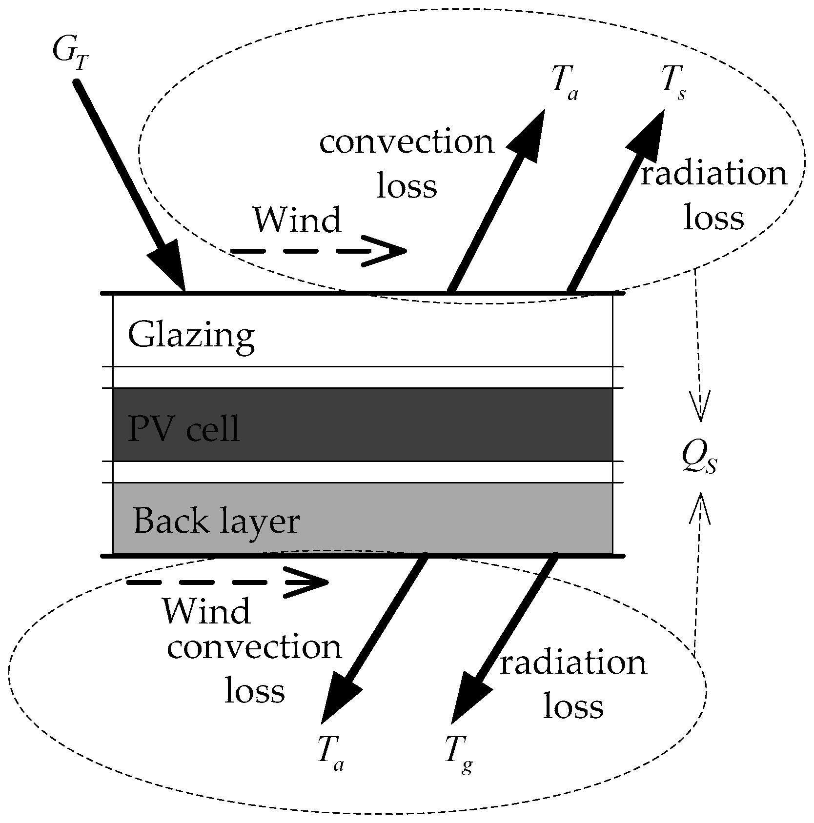
The schematic of the heat transfer process of the PV cell is shown in Figure 1, where Tg and Ts, are the temperature of ground and the temperature of sky, respectively. Here, Tg and Ts are all assumed to equal to Ta.
According to Newton’s law of cooling, the convective heat and irradiative transfer exchange from a surface to the surrounding fluid can be expressed in Equation (5):
Q S = h S ( T m T a ) = ( h r + h c ) S ( T m T a )
where h is heat transfer coefficient, hr and hc are heat transfer coefficient of radiation and heat transfer coefficient of convection, respectively. They are calculated according to Equations (6) and (7):
h r = ε σ ( T m + T a ) ( T m 2 + T a 2 )
h c = N u d / l
where ε is emissivity of materials, σ is Stefan-Boltzmann constant, d is air thermal conductivity, l is board length and Nu is Nusselt number.
For free cooling, if predominantly laminar flow is assumed, an approximation of Nu given by Holman can be expressed as Equation (8) [35]:
N u = 0.664 × P e 1 2 × P r 1 3
If it is the turbulent flow, the formula of Nu can be expressed as Equation (9) [35]:
N u = ( 0.037 × R e 4 5 871 ) × P r 1 3
where Pr is Prandtl number, and Re is the Reynolds number, which is used to characterize the flow of fluid, it is defined by Equation (10):
R e = V W S · l / ν
where VWS is the wind speed and ν is kinematic viscosity.
If we substitute Equations (6)–(10) into Equation (5), QS will be obtained as Equation (11) in the situation of laminar flow:
Q S = ε σ S ( T m 4 T a 4 ) + S ( T m T a ) 0.664 ( V W S · l / ν ) 1 2 P r 1 3 d / l
or as Equation (12) in the situation of turbulent flow:
Q S = ε σ S ( T m 4 T a 4 ) + S ( T m T a ) ( 0.037 ( V W S · l / ν ) 4 5 871 ) P r 1 3 d / l
Referring back to Equation (4), QS can be obtained through the above and we now turn to the module efficiency. Here we adopt the method given by Notton in 2005 [12]:
η = η r [ 1 β ( T m T a ) ]
where ηr is the reference value of PV module efficiency.
Finally, on the basis of σ being much smaller than Re, Tm is obtained in situation of laminar flow as Equation (14):
T m = 0.664 T a ( V W S · l / v ) 1 2 P r 1 3 d / l + α τ G T η r G T ( 1 + β T a ) 0.664 ( V W S · l / ν ) 1 2 P r 1 3 d / l η r β G T
or in situation of turbulent flow as Equation (15):
T m = T a ( 0.037 ( V W S · l / ν ) 4 5 871 ) 1 2 P r 1 3 d / l + α τ G T η r G T ( 1 + β T a ) ( 0.037 ( V W S · l / ν ) 4 5 871 ) P r 1 3 d / l η r β G T
From Equations (14) and (15), there are 11 impact factors of Tm:
(1) Five material/system-dependent factors: l, α, τ, ηr, and β.
Except for the structure parameter, l, the remaining four factors, α, τ, ηr, and β are performance parameters of the PV module, which can be obtained from the specifications of the PV module. These PV module parameters, which are constants for an already built PV plants, are dependent on the PV module technologies and encapsulation materials.
Three performance parameters of PV module can be decided by PV module technologies: α, ηr, and β. PV power plants usually use different PV module technologies, such as monocrystalline silicon (mc-Si), poly-silicon (p-Si), amorphous silicon (a-Si), and other thin film technologies such as copper indium diselenide (CIS), etc. [36]. In general, due to the advantages of crystalline silicon in the balance of energy conversion and the cost, the PV power plants applying this technology account for the largest proportion around the world, and dominate the PV market with around 90% share in 2014 [37,38]. When we refer to crystalline silicon, p-Si PV modules are normally cheaper, while mc-Si PV modules are more efficient, which means lager values of α and ηr.
The encapsulation materials are key characteristics of PV modules to determine the transmittance, τ, which is important in both the immediate and long-term power production of modules. Appropriate encapsulation materials can improve the optical flux transmittance, as well as protect the PV cell from the surroundings. The materials include ethylene vinyl acetate (EVA), polyvinyl butyral (PVB), poly dimethyl siloxane (PDMS), polyolefins, ionomers, and thermoplastic polyurethane (TPU) and so on [39]. Many encapsulation materials were found to discolor, with the resulting reduction in transmittance compromising PV module performance, so the transmittance of a PV module is influenced by thickness and durability of the encapsulation materials. However, there is no evidence for different encapsulation materials exhibiting much more different influence on transmittance in terms of same technology [39].
(2) Three surrounding-dependent factors: ν, Pr, k.
These three impact factors depend on the surroundings, especially ambient temperature. According to “Properties of Air at Atmospheric Pressure” in Heat Transfer written by Holman ([35], p. 643), the fitting relations between three factors and ambient temperature can be calculated as follows:
k = 7.559 × 10 5 T a + 0.02435
P r = 6.982 × 10 3 e ( T a 57.14 ) 2 × 9.309 × 10 5
ν = 1.024 × 10 7 T a + 1.336 × 10 5
It is obvious that at atmospheric pressure, the changes of the three factors only rely on ambient temperature, which also enhances the effect of ambient temperature on PV module temperature.
(3) Three MIFs: Ta, GT, and VWS.
Due to the characteristics of the above nine impact factors, when it comes to an already built PV plants, the changes of PV module temperature mainly rely on three MIFs: ambient temperature, solar irradiance and wind speed. According to Equations (14) and (15), the effects of ambient temperature and solar irradiance are almost proportional to the PV module temperature, while the effect of wind speed is in the form of fractional exponent power, which means the effect of wind speed is qualitatively weaker than the former two. Due to the fact the surroundings-dependent factors only rely on ambient temperature, from the angle of qualitative analysis, ambient temperature should be the most influential factor on PV module temperature, followed by solar irradiance, and wind speed is the weakest one.
The PV module temperature mainly relies on MIFs, which means the PV module temperature process will be different when the regulations of MIFs change. It is apparent that there are varying weather conditions, such as sunny days, cloudy days and so on [40], whose impacts on the PV module temperature can be grouped in two aspects: heat dissipation conditions and power generation performance. For example, on sunny days, solar irradiance and ambient temperature are stronger than on cloudy days, which will reduce the heat dissipation but enhance power generation, and finally, increase the PV module temperature. Thus, when we analyze the PV module temperature, the weather conditions should be classified to several types based on the distinction of three MIFs.
On the other hand, ambient temperature, solar irradiance and wind speed as MIFs of PV module temperature, are affected by each other. From a meteorological view, solar irradiance, as the main factor measuring the solar power, has a dominant impact on the ambient temperature changes on long-term time scale conditions or between different seasons other than a single day. It is the complexity and tight coupling between MIFs, which will bring redundancy to the researches and make quantitative analyses inaccurate, so mathematical methods relating PV module temperature and MIFs require further research.

3. Mathematical Foundation

Based on the earlier physical analysis, the distinguishing features of MIFs of PV module temperature can be summarized by the following aspects: diversity; complexity and cross coupling, so in order to analyse MIFs quantitatively, several statistical methods should be utilized. CFS, given by Hall [41], is an available method based on correlation coefficient calculation to measure the correlation degree between impact factors and PV module temperature, which provides a basis for the specific degrees of influence of different factors on PV module temperature [26]. MI, given by Mackay [42], is based on measuring the same information among different variables. It is a measure of relevance and redundancy between variables, which can weigh the influence degrees as well [43]. On that basis, two methods, which are linear and nonlinear, respectively, are adopted to describe and compare the impact of MIFs on PV module temperature quantitatively as follows.

3.1. Correlation-Based Feature Selection

Given the target variable is Z and selected subset is C, CFS is defined as the following equation:
r C Z = k r i Z ¯ / k + k ( k 1 ) r i i ¯
where rcz is the correlation between the Z and C, k is the number of features, riZ and rii are the correlation coefficient between each feature in C and Z and the correlation coefficient between each feature in C. The correlation coefficient can be calculated as Equation (20):
r = i = 1 n ( x i x ¯ ) ( y i y ¯ ) / i = 1 n ( x i x ¯ ) 2 i = 1 n ( y i y ¯ ) 2
where n is the number of data in a variable, xi and yi are the data in feature subsets and target variable respectively.
CFS is a linear method measuring the relevance to find the best possible variable C by maximizing the rsz, in which process the best relevant set of MIFs will be selected. Since the dimension of candidate features maybe high, the time consumption cannot be neglected [26]. We adopt a greedy stepwise search algorithm to find a best C starting with a small set of definite features and adding one another feature at one time [44], and only if the data of rsz increases, the new feature will be accepted, and until there is no improvement or no features to add, it stops to identify the most relevant subset which contains the major relevant factors of PV module temperature.

3.2. Mutual Information

MI based on information entropy is a nonlinear method to measure the relevance and redundancy between variables, in which entropy is a measurement of uncertainty of each variable, while MI calculates the same information in two variables [45].
Given the random feature variable X is X = (x1, x2, …, xN), entropy information H(X) is defined as Equation (21):
H ( X ) = i = 1 n p i log p i
where pi is the probability of xi with value between xi,p and xi,p+1,which means that x is needed to divided into several segments in advance. Here we determine the segment number is k. pi is defined as Equation (22):
p i = number   of   x   with   value   in   [ x i , p , x i . p + 1 ] total   number   of   data   in   x i   subset
For any two random variables X and Y, the two-dimensional joint entropy is defined as Equation (23):
H ( X , Y ) = i = 1 n j = 1 m p i j log p i j
Furthermore, the conditional entropy probability represents the amount of uncertainty in one of variables when the other one is introduced, in which pij is the probability of x and y with value in [xi,p, xi,p+1] and [yi,q, yi,q+1], as shown in Equations (24)–(26):
H ( X | Y ) = i = 1 n j = 1 m p i j log p i j p j
H ( Y | X ) = i = 1 n j = 1 m p i j log p i j p i
p i j = number   of   ( x , y ) with   value   [ x i , p ,   x i , p + 1 ]   and   [ y j , q , y j , q + 1 ]   total   number   of   ( x , y )
The relationship between joint entropy and conditional entropy is defined as Equation (27):
H ( X , Y ) = H ( X ) + H ( Y | X ) = H ( Y ) + H ( X | Y )
Thus, MI expressing the information shared in both variables is defined as Equation (28):
I ( X ; Y ) = I ( Y ; X ) = H ( X ) H ( X | Y ) = H ( Y ) H ( Y | X ) = H ( X ) + H ( Y ) H ( X , Y )
Conditional mutual information (CMI) reflects the MI between features that has not been selected and the target variable Z with several features that has been determined, as Equation (29) shown:
I ( X ; Z | Y ) = H ( X | Y ) H ( X | Z , Y ) = y Y p ( y ) x X y Y p ( x , z | y ) log p ( x , z | y ) p ( x | y ) p ( z | y )
The joint mutual information (JMI) is defined as:
I ( X , Y ; Z ) = I ( X ; Z | Y ) + I ( Y ; Z )
So the interaction information (II) between X, Y and Z is:
I ( X ; Y ; Z ) = I ( X ; Z ) + I ( Y ; Z ) I ( X , Y ; Z )
The Venn diagram, a presentation of concepts of H, MI, CMI JMI and II, is provided for visual explanation of each method, as Figure 2 shows [46].
Each area in Figure 2 expresses respectively:
  • The circles: H values range of variables;
  • The union of area 3 and 4: I(X; Y), MI;
  • The area 1: I(X; Z|Y), CMI;
  • The union of area 1, 2 and 4: I(X, Y; Z), JMI;
  • The area 4: I(X; Y; Z), II.
As shown in Figure 2, the value of H represents the variable uncertainty, which also means the information contained in this variable. MI reflects the relevant information between two variables, while II expresses the redundant information in three variables, so the values of H, MI and II can be utilized in the quantitative measurements of relevancy and redundancy between MIFs and PV module temperature, and these indexes based on MI theory are selected to explore the specific degree of impact under varying typical weather statuses.

4. Quantitative Degree of Influence of Meteorological Impact Factors on Photovoltaic Module Temperature

4.1. Data

The dataset used to carry out this research, covering the time range from January 2012 to December 2012, comes from a 500 kW grid-connected PV plant in China connecting the grid through a voltage level of 6 kV, which includes the variables of solar irradiance (GT), ambient temperature (Ta), and wind speed (
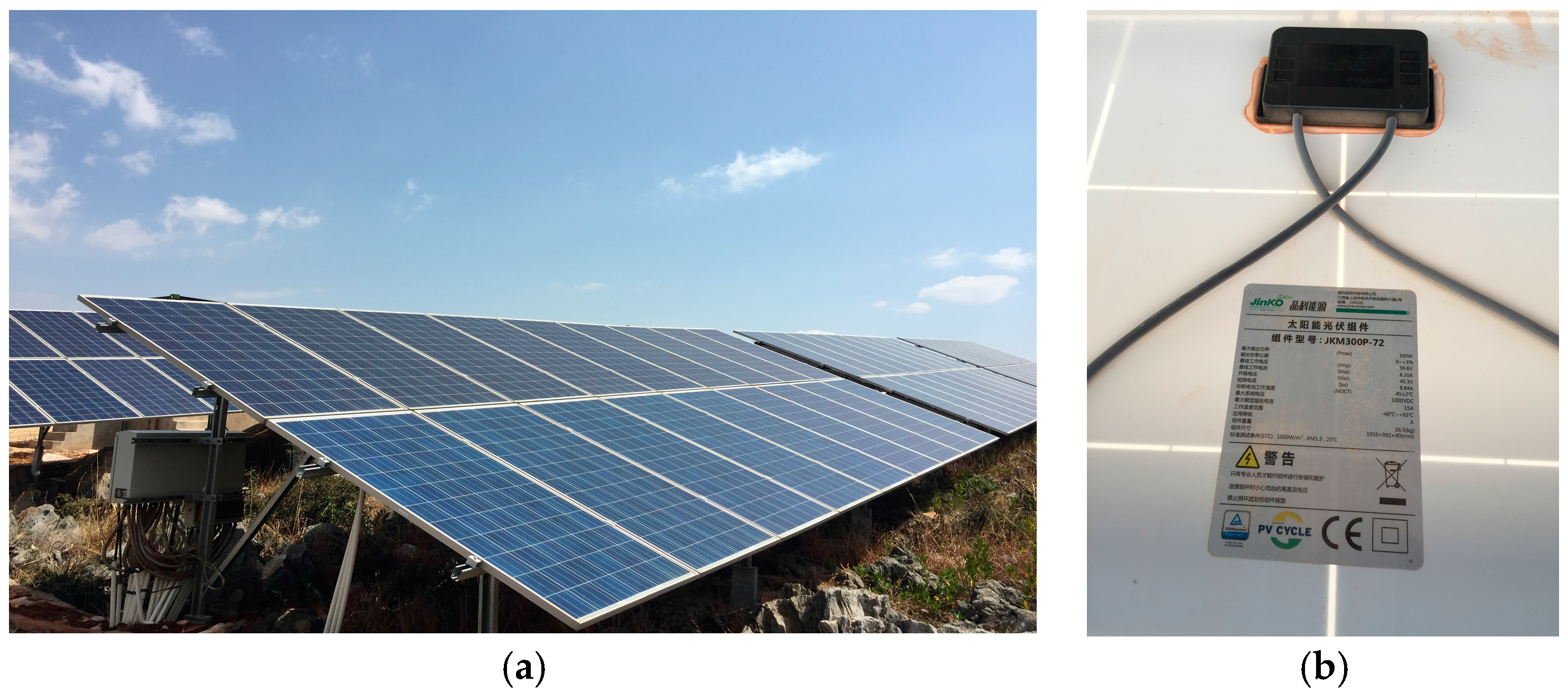
VWS) with the time interval of 30 min. The annual total available records cover 310 days during the whole year. The manufacturer of the PV module installed in this plant is JinKo Solar Company (Shangrao, Jiangxi, China) and the assembly model is JKMS300P-72 adopting p-Si technology, which can be seen in Figure 3. The total number of PV cells in each module is 72 (6 × 12). The size of each cell is 156 mm × 156 mm. The parameters of the JKM300P-72 PV module are listed in Table 1, where NOCT means normal operating cell temperature. The models and parameters of the sensors deployed in this plant are listed in Table 2.
The analysis work is conducted only during the daytime period with sunlight because the purpose of this research is to try to help improve the solar PV power forecasting through making clear the influence of MIFs on PV module temperature. More importantly, due to heat transfer, PV module temperature is appropriately the same as the ambient temperature, which means the MIFs are different during the day and night. Therefore, although the temperature data is continuous in a whole day, we select the data from 7:00 a.m. to 5:00 p.m. to conduct the mathematical analysis, i.e., 20 data points per day are selected for the case study.
As mentioned above in Section 1 and Section 2 of this paper, weather conditions have significant impacts on the heat dissipation conditions of PV modules. “GB/T 22164-2008 Public Climate Service—Weather Graphic Symbols” released by China Meteorological Administration defined 33 types of weather status [47]. In order to balance the accuracy and complexity of the analysis of PV module temperature, the numbers of weather types should be reasonable and the summative weather statuses should be typical and representative. Summarizing the most vital characteristics of all climates, the weather statuses can generally be divided into four typical different classes: sunny day, cloudy day, shower day and heavy rainy day [32]. Furthermore, the other weather statuses are assigned to one of these four classes according to the degree of closeness described by a correlation coefficient, and then four general weather classes (GWCs) named A, B, C, and D are constituted [40]. After removing the invalid data, the distribution of four different GWCs are 24, 119, 148, and 19 days, respectively.
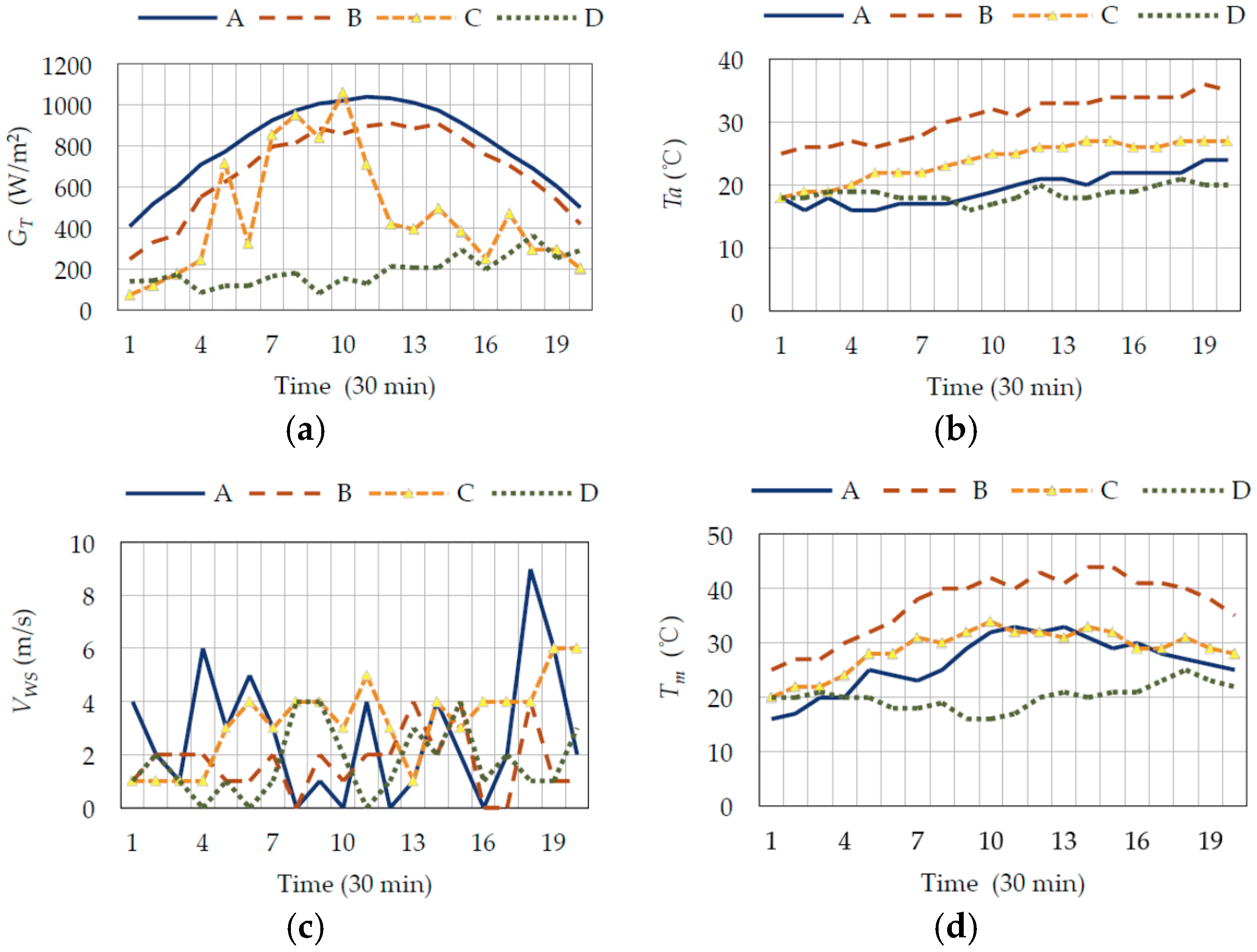
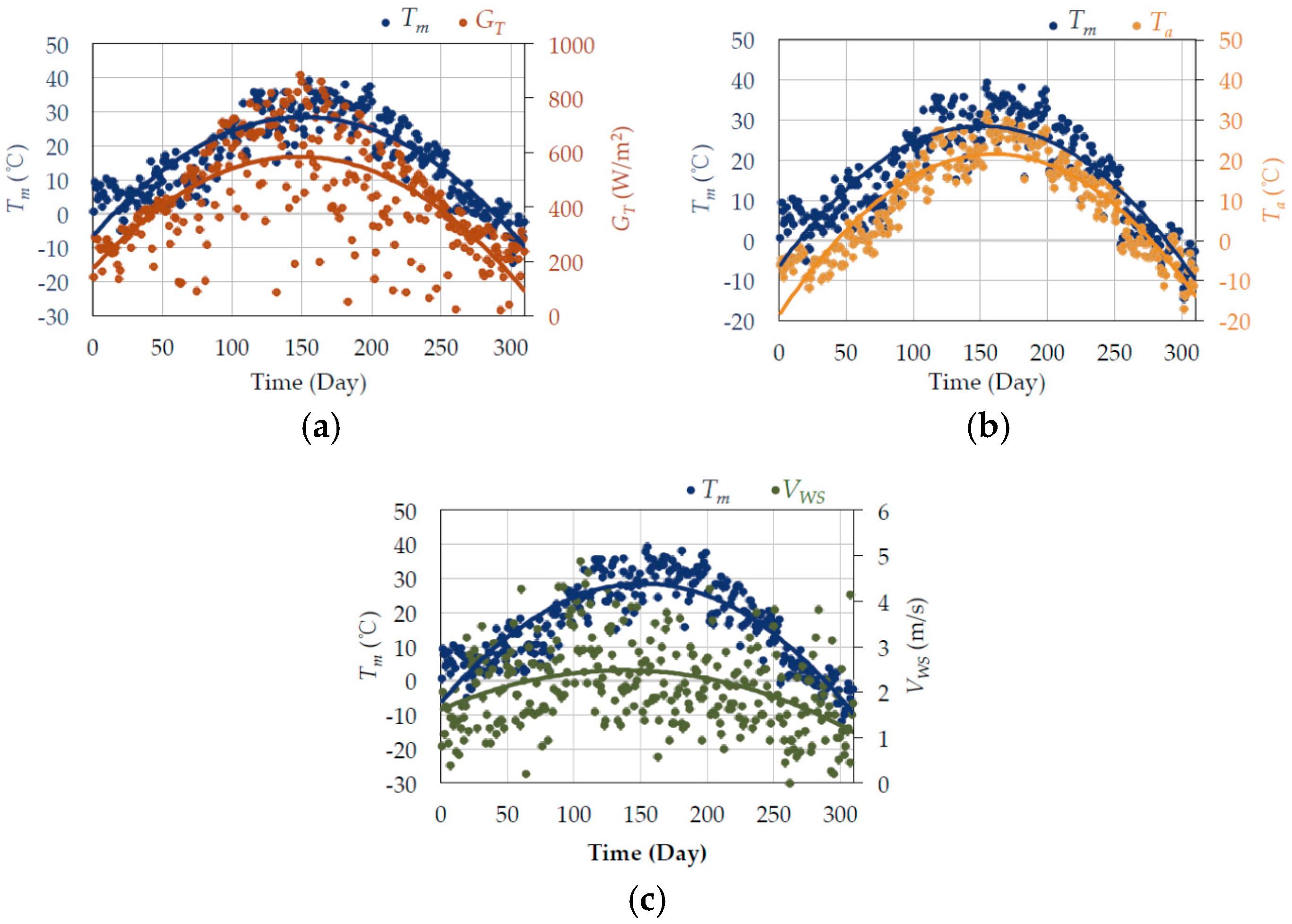
Figure 4 is the actual data of PV module temperature and its MIFs on a certain day under four GWCs. The dates selected to represent the rules of four GWCs are 10 June, 18 June, 24 June, and 6 June respectively. It is shown that the changes of PV module temperature are the common interaction among all three MIFs. For example, in weather class A, although the solar irradiance is much stronger, the ambient temperature is lower and the wind speed is bigger than in other classes, so the PV module temperature is not very high.
Furthermore, we take the averages of the PV module temperature and its MIFs on each day to draw Figure 5 to make further observation on the correlation relations.
Figure 6 is the actual data of PV module temperature in the whole year under four GWCs. The PV module temperature data show a strip distribution, which is caused by the temperature difference of about 20 °C per day, but as a whole, it is in accord with the seasonal characteristics.

4.2. Quantitative Correlation Analysis by Correlation-Based Feature Selection

Figure 5 shows that the positive relation between ambient temperature and PV module temperature is more obvious than the other two impact factors, but whether the change trend is similar to the trend of impact degrees merits quantitative study. CFS provides a possibility for quantitative analysis for PV module temperature. The quantitative relations in four GWCs between MIFs and PV module temperature measured by correlation coefficients are shown in Table 3.
Furthermore, the ratios of quantitative influence degrees of these three MIFs under four GWCs measured by correlation coefficients are shown as Table 4.
It shows that in four GWCs, the ambient temperature has the strongest correlation with PV module temperature, followed by solar irradiance, and wind speed is the weakest influential factor on PV module temperature. The quantitative ratio of influence degrees of these three MIFs measured by correlation coefficients are 50:40:10, 45:42:13, 50:38:12 and 52:29:19, respectively, under four GWCs. When we focus on only one factor, such as solar irradiance, the ratios of four GWCs are 40%, 42%, 38% and 29%, which are different in different weather classes. The reason is that the classification of weather types is based on the differences of the meteorological factors, which in turn meteorological factors perform differently in different weather classifications. For heavy rainy days (weather class D), solar irradiance is the lowest and the changes are very small, which is the reason why the effect of solar irradiance becomes less in weather class D.
The values of rcz are calculated based on the correlation coefficients, and the results are shown in Table 5. According to the analysis above, the correlation coefficients between ambient temperature and PV module temperature are the highest under four GWCs, so we put Ta in the C set firstly, and add one another impact feature at one time.
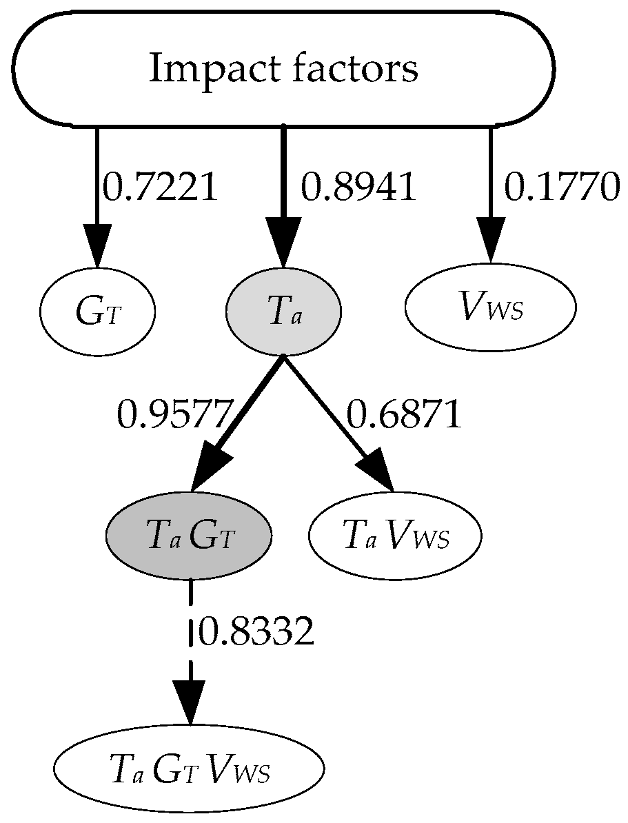
Besides putting only one factor or all three factors as the study object, the combination of two variables also has the opportunity to become the most influential subset. The process of selection by rsz is presented in Figure 7 with the example in weather class A: firstly, determining C = {Ta}, secondly, adding GT and VWS into the C set, comparing the rcz values of {Ta, GT} and {Ta, VWS} with original rcz value, and choosing the new set with increased rcz values: {Ta, GT}, thirdly, adding VWS into {Ta, GT}, and repeating the previous step. The final result shows that in weather class A, the combination of GT and Ta is the most relevant subset with Tm. Table 6 shows the other most relevant subsets with Tm in four GWCs.
It is evident that Ta is the most influential factor in all kinds of weather classifications, and GT is a primary impact factor, except in weather class D, while VWS is not primarily relevant to Tm. Like in the analysis above, in weather class D, solar irradiance is lower and changes little, which makes it have little effect in this GWCs.
The result analyzed by CFS verifies the physical analysis results. However, the correlation coefficient values cannot express the degree of relevance exactly because the correlation coefficient is a linear value while the relationship between Tm and each impact factor is nonlinear. More importantly, the relevant subsets contain a certain degree of redundant information due to the coupling relation between MIFs. Thus, the nonlinear method, MI is worthy of further research.

4.3. Quantitative Correlation Analysis by Mutual Information Theory

The MI of two random variables is a measure of the mutual dependence between the two variables. More specifically, it quantifies the “amount of information” obtained about one random variable, through the other random variable. According to Equation (22), k as the number of data segments, determines the intricacy of the study. If k is larger, the data is divided more detailed, and each part of data range is smaller, which will lead the sample distribution more discrete, so in this case, the entropy information and MI are larger generally. If k is smaller, the entropy information and MI are smaller generally. Thus, what is the premise of accurate reflection of nonlinear coupling relation is a reasonable k value.
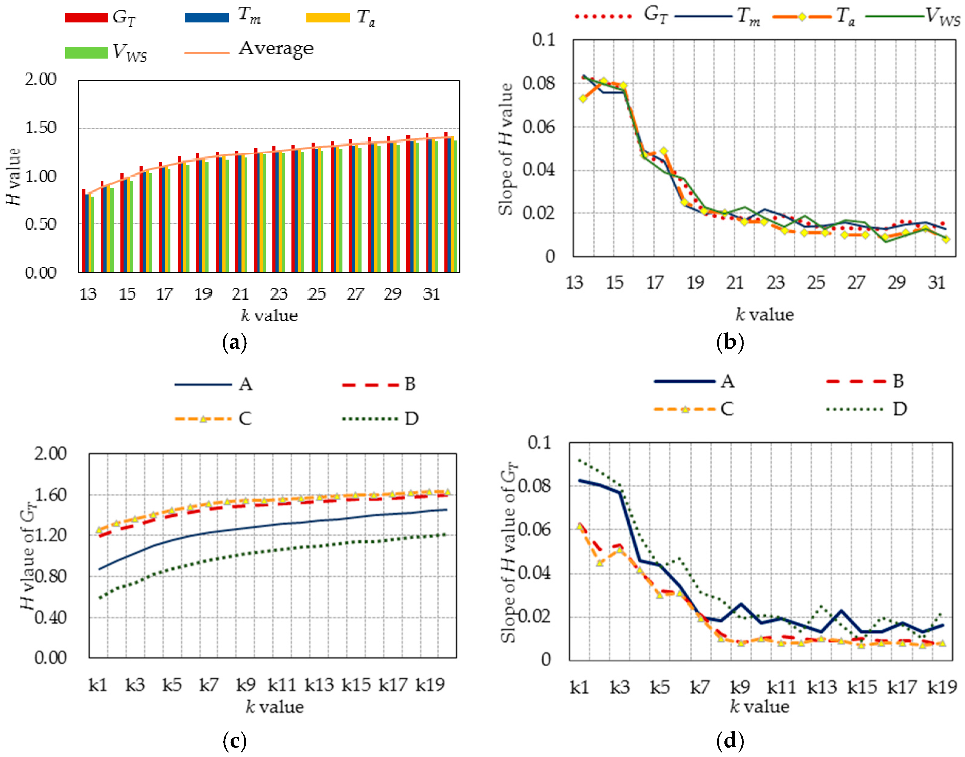
In order to achieve a scientific and reasonable k value, accuracy and complexity need to be considered. Due to the fact there is no mathematical method to determine k values, a method based on actual data is applied in this paper. Firstly, a range values set of k are determined. Secondly, the tendency of the average value of H is observed to find the reasonable k value after the H values of all variables are calculated. Let’s take the weather class A as an example. As shown in Figure 8a, the H values of four variables are calculated with k between 13 and 32 in weather class A. The slope values of the H values are shown in Figure 8b, in which the tendency is more clear. It is obvious that when the k value reaches 20, the slope values tend to be constant, which is the k value that should be selected. As a result, the k values in weather class A is determined as 20. Figure 8a,b both indicates that the H values of different variables are similar in the same weather classes, so we choose one of four variables to study k values in the other three GWCs. The H values of GT in four GWCs with different k values are shown in Figure 8c, and Figure 8d is the slope value of the above data. What is noteworthy is that the set of k values in different weather classifications is different, which means that ki reflects different values in different weather classification. The value ranges of k value in weather class B, C and D are between 33 and 52, 37 and 56, 11 and 30, respectively. Similarly, according to our definition, the k values in weather classes B, C and D are 40, 44 and 18, respectively.
With the identified k values, according to Equations (21) and (23), entropy information (H(X)) and joint entropy (H(X, Y)) can be calculated. The results are shown in Table 7 and Table 8.
According to Equation (28), the MI (I(X, Y)) is obtained on the basic of entropy information and joint entropy. 
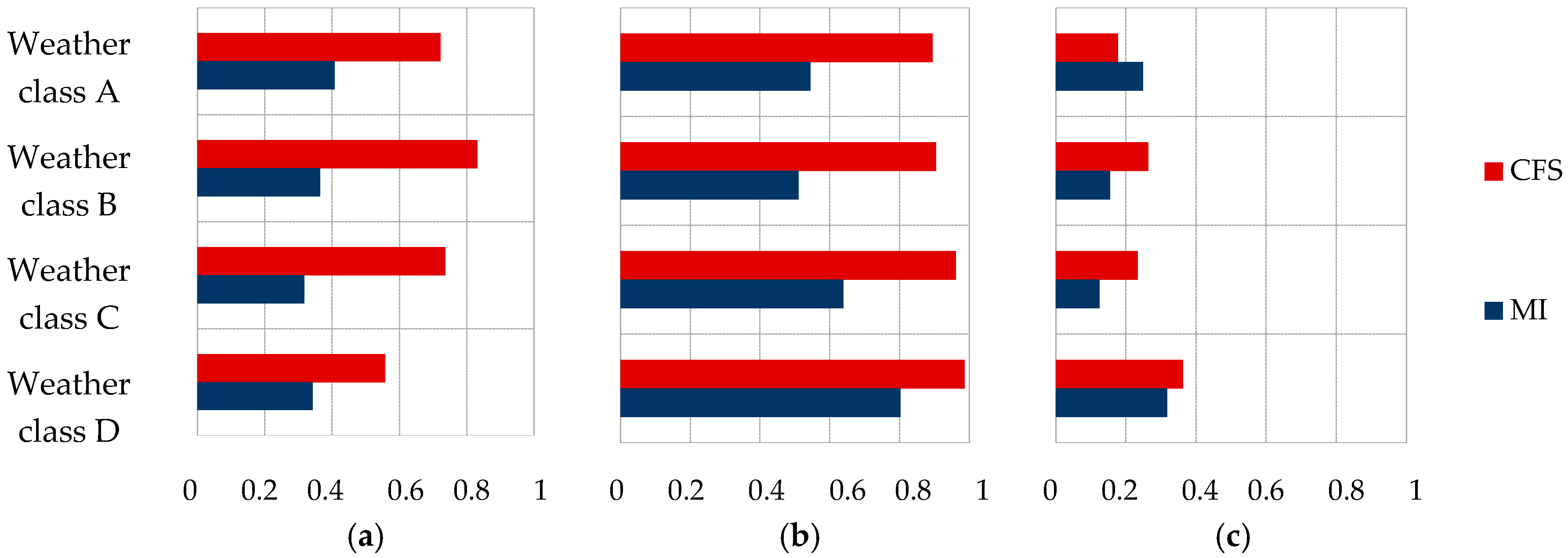
Table 9 is the MI between three MIFs and PV module temperature. MI and correlation coefficient are two methods to measure the relevance between two variables. When we compare Table 9 with Table 3, the correlation coefficient values are larger than the values of MI, shown as Figure 9.
The reason is that CFS is a linear method, which will neglect the coupling relation between MIFs, so the degree of influence of each MIF on PV module temperature is enhanced, which contains redundancy between MIFs, while MI takes the interaction with other factors into consideration, which will reduce the effect of this single impact factor. Thus, MI is more precise in quantitative research on MIFs of PV module temperature.
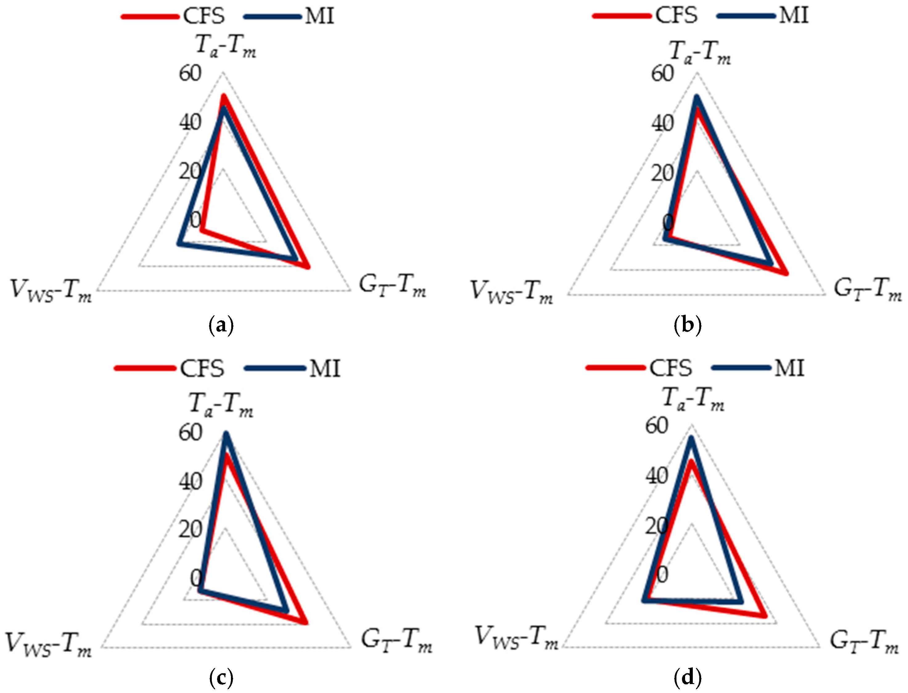
Table 10 shows the ratios of MI between MIFs and PV module temperature under four GWCs and the ratios of relevancy of these three MIFs measured by MI are 34:45:21, 35:50:15, 29:59:12, and 23:55:22, respectively, under four GWCs. Furthermore, the results measured by two mathematical methods are compared with each other, shown as Figure 10.
The comparative results show several commonalities. Firstly, the monotone increasing order of the degrees of influence of the three MIFs in four GWCs is: Ta, GT, and VWS. Secondly, the relation between solar irradiance and PV module temperature (GT-Tm) measured by MI is smaller than the value measured by CFS, while the relation between wind speed and PV module temperature (VWS-Tm) is similar or larger. The decreasing ratios of solar irradiance are mainly due to the increasing redundancy between ambient temperature and solar irradiance and MI can eliminate the influence of redundancy, while CFS cannot.
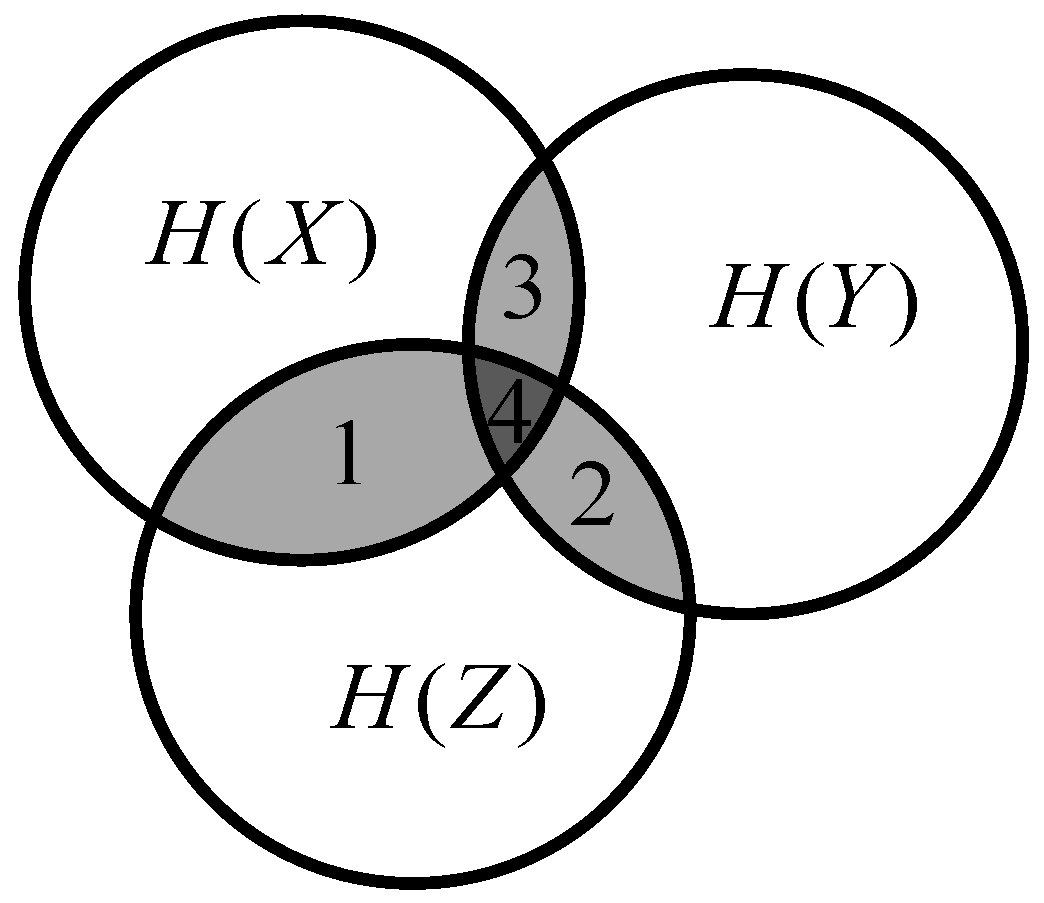
Furthermore, how much redundancy existed between each MIF is also addressed. According to Equations (30) and (31), the values of II can measure the redundancy between two variables when they act on the same object, which is shown in Table 11.
The ratio of quantitative redundancy degrees is shown in Table 12. It is worth noticing that:
p ( x | y ) = p ( x y ) / p ( y )
and:
p ( x , z | y ) = p ( x y z ) / p ( x y )
The ratios of quantitative redundancy degrees between Ta and GT, Ta and VWS, GT and VWS are 61:28:11, 57:30:13, 62:26:12, and 62:33:5, respectively, under four GWCs. The redundancy between solar irradiance and ambient temperature is highest in three variables, which is caused by the significant effect of solar irradiance to ambient temperature. Wind speed also influences the ambient temperature by accelerating heat transfer, which reflects in the higher values of I(Ta; VWS; Tm). Wind speed and solar irradiance have little redundancy relation.

5. Conclusions

Quantitative methods based on CFS and MI theory to describe the degree of influence of MIFs on PV module temperature are proposed after the interdisciplinary theory analysis using correlation analysis, PV material and heat transfer theory. A case study is conducted using the actual data from January 2012 to December 2012 of a 500 kW grid-connected PV power plant in China. The mathematical quantitative degree of correlation between MIFs and PV module temperature were simulated, analyzed and compared under the cases of four actual different weather conditions named as GWCs. The results obtained can be summarized as follows:
(1)
Generally, there are 12 impact factors of PV module temperature, which can be divided into three categories, i.e., six material/system-dependent factors, three surroundings-dependent factors, and three MIFs.
(2)
Material/system-dependent factors are depended on PV module technologies and encapsulation materials, and surroundings-dependent factors rely on MIFs, especially ambient temperature, while MIFs have complexity and tight coupling with each other and show discrepancies in different weather statuses.
(3)
In an existing PV plant, the changes of PV module temperature mainly rely on three MIFs: ambient temperature, solar irradiance and wind speed.
(4)
The ratios of quantitative degrees of influence of these three MIFs measured by correlation coefficient are 50:40:10, 45:42:13, 50:38:12 and 52:29:19, respectively, under four GWCs.
(5)
The ratios of quantitative influence degrees of these three MIFs measured by MI are 45:34:21, 50:35:15, 59:29:12, and 53:23:22, respectively, under four GWCs.
(6)
The ratios of quantitative redundancy degrees between Ta and GT, Ta and VWS, GT and VWS are 61:28:11, 57:30:13, 62:26:12, and 62:33:5, respectively, under four GWCs.
We can confirm the key MIFs of PV module temperature and then address the influence and degrees of redundancy quantitatively based on this research, which will help us to improve PV module temperature predictions and provide a potential foundation to enhance the accuracy of solar PV power forecasting. For example, it is very important for classification modeling of solar PV forecasting to consider the specific influences of multiple MIFs clearly under different weather conditions. The specific quantitative values of influence and degrees of redundancy probably will be different from this paper when the environment conditions or locations of PV plants are changed. Future studies on this topic will focus on discerning the applicability of the proposed methods for other different PV plants, and the authors hope to undertake work on this topic not only in China but also internationally.

Acknowledgments

This work was supported in part by the National Natural Science Foundation of China (51577067, 51277075); the Natural Science Foundation of Beijing (3162033); the Natural Science Foundation of Hebei Province (E2015502060); the Key Project of the Science and Technology Support Program of Hebei Province (12213913D); the Fundamental Research Funds for the Central Universities (2014ZD29 and 2015XS108); State Key Laboratory of Alternate Electrical Power System with Renewable Energy Sources (LAPS15009, LAPS16007 and LAPS16015), the China Scholarship Council (CSC) and the Science & Technology Project of State Grid Corporation of China (SGCC).

Author Contributions

Fei Wang and Zengqiang Mi conceived and designed the experiments; Yujing Sun performed the experiments; Yujing Sun analyzed the data; Qifang Chen, N.A. Engerer and Bo Wang contributed reagents/materials/analysis tools; Yujing Sun and Fei Wang wrote the paper.

Conflicts of Interest

The authors declare no conflict of interest. The founding sponsors had no role in the design of the study; in the collection, analyses, or interpretation of data; in the writing of the manuscript, and in the decision to publish the results.

References

  1. International Energy Agency (IEA). Energy Policies of IEA Countries—Portugal 2016 Review; International Energy Agency (IEA): Paris, France, 2016. [Google Scholar]
  2. International Energy Agency (IEA). World Energy Outlook Special Report 2015: Energy and Climate Change; International Energy Agency (IEA): Paris, France, 2015. [Google Scholar]
  3. Akinyele, D.O.; Rayudu, R.K.; Nair, N.K.C. Global progress in photovoltaic technologies and the scenario of development of solar panel plant and module performance estimation—Application in Nigeria. Renew. Sustain. Energy Rev. 2015, 48, 112–139. [Google Scholar] [CrossRef]
  4. International Energy Agency (IEA). Snapshot of Global Photovoltaic Markets 2015; International Energy Agency (IEA): Paris, France, 2015. [Google Scholar]
  5. Skoplaki, E.; Palyvos, J.A. On the temperature dependence of photovoltaic module electrical performance: A review of efficiency/power correlations. Sol. Energy 2009, 83, 614–624. [Google Scholar] [CrossRef]
  6. International Energy Agency (IEA). Renewable Energy Technologies: Solar Energy Perspectives; International Energy Agency (IEA): Paris, France, 2011. [Google Scholar]
  7. Kawabe, K.; Tanaka, K. Impact of dynamic behavior of photovoltaic power generation systems on short-term voltage stability. IEEE Trans. Power Syst. 2015, 30, 3416–3424. [Google Scholar] [CrossRef]
  8. Shaker, H.; Zareipour, H.; Wood, D. Impacts of large-scale wind and solar power integration on California’s net electrical load. Renew. Sustain. Energy Rev. 2016, 58, 761–774. [Google Scholar] [CrossRef]
  9. Zhang, J.; Florita, A.; Hodge, B.M.; Lu, S.Y.; Hamann, H.F.; Banunarayanan, V.; Brockway, A.M. A suite of metrics for assessing the performance of solar power forecasting. Sol. Energy 2015, 111, 157–175. [Google Scholar] [CrossRef]
  10. Osório, G.J.; Lujano-Rojas, J.M.; Matias, J.C.O.; Catalão, J.P.S. A probabilistic approach to solve the economic dispatch problem with intermittent renewable energy sources. Energy 2015, 82, 949–959. [Google Scholar] [CrossRef]
  11. Brano, V.L.; Ciulla, G.; Piacentino, A.; Cardona, F. On the efficacy of PCM to shave peak temperature of crystalline photovoltaic panels: An FDM model and field validation. Energies 2013, 12, 6188–6210. [Google Scholar] [CrossRef] [Green Version]
  12. Mattei, M.; Notton, G.; Cristofari, C.; Muselli, M.; Poggi, P. Calculation of the polycrystalline PV module temperature using a simple method of energy balance. Renew. Energy 2006, 31, 553–567. [Google Scholar] [CrossRef]
  13. Jakhrani, A.Q.; Othman, A.K.; Rigit, A.R.H.; Samo, S.R. Determination and comparison of different photovoltaic module temperature models for Kuching, Sarawak. In Proceedings of the IEEE First Conference on Clean Energy and Technology (CET), Kuala Lumpur, Malaysia, 27–29 June 2011.
  14. Fernández, E.F.; Almonacid, F.; Sarmah, N.; Rodrigo, P.; Mallick, T.K.; Perez-Higueras, P. A model based on artificial neuronal network for the prediction of the maximum power of a low concentration photovoltaic module for building integration. Sol. Energy 2014, 100, 148–158. [Google Scholar] [CrossRef]
  15. Huld, T.; Amillo, A. Estimating PV module performance over large geographical regions: The role of irradiance, air temperature, wind speed and solar spectrum. Energies 2015, 8, 5159–5181. [Google Scholar] [CrossRef] [Green Version]
  16. Mellit, A.; Pavan, A.M.; Lughi, V. Short-term forecasting of power production in a large-scale photovoltaic plant. Sol. Energy 2014, 105, 401–413. [Google Scholar] [CrossRef]
  17. Chenni, R.; Makhlouf, M.; Kerbache, T.; Bouzid, A. A detailed modeling method for photovoltaic cells. Energy 2007, 32, 1724–1730. [Google Scholar] [CrossRef]
  18. Veldhuis, A.J.; Nobre, A.M.; Peters, I.M.; Reindl, T.; Ruther, R.; Reinders, A.H.M.E. An empirical model for rack-mounted PV module temperatures for Southeast Asian locations evaluated for minute time scales. IEEE J. Photovolt. 2015, 5, 774–782. [Google Scholar] [CrossRef]
  19. Park, K.E.; Kang, G.H.; Kim, H.I.; Yu, G.J.; Kim, J.T. Analysis of thermal and electrical performance of semi-transparent photovoltaic (PV) module. Energy 2010, 35, 2681–2687. [Google Scholar] [CrossRef]
  20. Routh, T.K.; Yousuf, A.H.B.; Hossain, M.N.; Asasduzzaman, M.M.; Hossain, M.I.; Husnaeen, U.; Mubarak, M. Artificial neural network based temperature prediction and its impact on solar cell. In Proceedings of the 2012 International Conference on Informatics, Electronics & Vision (ICIEV), Dhaka, Bangladesh, 18–19 May 2012.
  21. Peng, J.; Lu, L.; Yang, H.; Ma, T. Comparative study of the thermal and power performances of a semi-transparent photovoltaic façade under different ventilation modes. Appl. Energy 2015, 138, 572–583. [Google Scholar] [CrossRef]
  22. Skoplaki, E.; Palyvos, J.A. Operating temperature of photovoltaic modules: A survey of pertinent correlations. Renew. Energy 2009, 34, 23–29. [Google Scholar] [CrossRef]
  23. Wang, F.; Mi, Z.; Su, S.; Zhao, H. Short-term solar irradiance forecasting model based on artificial neural network using statistical feature parameters. Energies 2012, 12, 1355–1370. [Google Scholar] [CrossRef]
  24. Koprinska, I.; Rana, M.; Agelidis, V.G. Yearly and seasonal models for electricity load forecasting. In Proceedings of the International Joint Conference on Neural Networks (IJCNN), San Jose, CA, USA, 31 July–5 August 2011; pp. 1474–1481.
  25. Koprinska, I.; Sood, R.; Agelidis, V.G. Variable selection for five-minute ahead electricity load forecasting. In Proceedings of the 20th International Conference on Pattern Recognition (ICPR), Istanbul, Turkey, 23–26 August 2010; pp. 2901–2904.
  26. Koprinska, I.; Rana, M.; Agelidis, V.G. Correlation and instance based feature selection for electricity load forecasting. Knowl.-Based Syst. 2015, 82, 29–40. [Google Scholar] [CrossRef]
  27. Xu, R.; Taubman, D.; Naman, A.T. Motion estimation based on mutual information and adaptive multi-scale thresholding. IEEE Trans. Image Process. 2016, 25, 1095–1108. [Google Scholar] [CrossRef] [PubMed]
  28. Jaesung, L.; Kim, D.W. Mutual information-based multi-label feature selection using interaction information. Expert Syst. Appl. 2014, 42, 2013–2025. [Google Scholar]
  29. Lin, Y.; Hu, Q.; Liu, J.; Duan, J. Multi-label feature selection based on max-dependency and min-redundancy. Neurocomputing 2015, 168, 92–103. [Google Scholar] [CrossRef]
  30. Renani, E.T.; Elias, M.F.M.; Rahim, N.A. Using data-driven approach for wind power prediction: A comparative study. Energy Convers. Manag. 2016, 118, 193–203. [Google Scholar] [CrossRef]
  31. Li, Z.; Mahbobur Rahman, S.M.; Vega, R.; Dong, B. A hierarchical approach using machine learning methods in solar photovoltaic energy production forecasting. Energies 2016, 9, 55. [Google Scholar] [CrossRef]
  32. Sun, Y.; Wang, F.; Zhen, Z.; Mi, Z.; Liu, C.; Wang, B.; Lu, J. Short-term prediction model of module temperature for photovoltaic power forecasting based on support vector machine. In Proceedings of the International Conference on Renewable Power Generation (RPG 2015), Beijing, China, 17–18 October 2015.
  33. Sun, Y.; Wang, F.; Zhen, Z.; Mi, Z.; Sun, H.; Liu, C.; Wang, B.; Lu, J.; Zhen, Z.; Li, K. Research on short-term module temperature prediction model based on BP neural network for photovoltaic power forecasting. In Proceedings of the 2015 IEEE Power & Energy Society General Meeting, Denver, CO, USA, 26–30 July 2015.
  34. Xavier, G.A.; Filho, D.O.; Martins, J.H.; Marcos, D.B.M.P. Simulation of distributed generation with photovoltaic microgrids—Case study in Brazil. Energies 2015, 8, 4003–4023. [Google Scholar] [CrossRef]
  35. Holman, J.P. Heat Transfer, 9th ed.; McGraw-Hill: New York, NY, USA, 2002. [Google Scholar]
  36. Calise, F.; Vanoli, L. Parabolic trough photovoltaic/thermal collectors: Design and simulation model. Energies 2012, 5, 4186–4208. [Google Scholar] [CrossRef]
  37. Edalati, S.; Ameri, M.; Iranmanesh, M. Comparative performance investigation of mono- and poly-crystalline silicon photovoltaic modules for use in grid-connected photovoltaic systems in dry climates. Appl. Energy 2015, 160, 255–265. [Google Scholar] [CrossRef]
  38. International Energy Agency (IEA). Technology Roadmap: Solar Photovoltaic Energy—2014 Edition; International Energy Agency (IEA): Paris, France, 2014. [Google Scholar]
  39. Miller, D.C.; Muller, M.T.; Kempe, M.D.; Araki, K.; Kennedy, C.E.; Kurtz, S.R. Durability of polymeric encapsulation materials for concentrating photovoltaic systems. Prog. Photovolt. 2013, 4, 631–651. [Google Scholar] [CrossRef]
  40. Wang, F.; Zhen, Z.; Mi, Z.; Sun, H.; Su, S.; Yang, G. Solar irradiance feature extraction and support vector machines based weather status pattern recognition model for short-term photovoltaic power forecasting. Energy Build. 2015, 86, 427–438. [Google Scholar] [CrossRef]
  41. Hall, M.A. Correlation-Based Feature Selection for Machine Learning. Ph.D. Thesis, The University of Waikato, Hamilton, New Zealand, 1999. [Google Scholar]
  42. MacKay, D.J.C. Information Theory, Inference and Learning Algorithms; Cambridge University Press: Cambridge, UK, 2003. [Google Scholar]
  43. Brown, G.; Pocock, A.; Zhao, M.; Lujan, M. Conditional likelihood maximization: A unifying framework for information theoretic feature selection. J. Mach. Learn. Res. 2012, 13, 27–66. [Google Scholar]
  44. Han, M.; Ren, W. Global mutual information-based feature selection approach using single-objective and multi-objective optimization. Neurocomputing 2015, 168, 47–54. [Google Scholar] [CrossRef]
  45. Qian, W.; Shu, W. Mutual information criterion for feature selection from incomplete data. Neurocomputing 2015, 168, 210–220. [Google Scholar] [CrossRef]
  46. Bennasar, M.; Hicks, Y.; Setchi, R. Feature selection using joint mutual information maximisation. Expert Syst. Appl. 2015, 42, 8520–8532. [Google Scholar] [CrossRef]
  47. China Meteorological Administration. GB/T 22164—2008 Public Climate Service—Weather Graphic Symbols; Standards Press of China: Beijing, China, 2008.
Figure 1. Schematic of the thermal processes of a photovoltaic (PV) cell.
Energies 10 00007 g001
Figure 2. Venn diagrams of mutual information (MI).
Energies 10 00007 g002
Figure 3. The PV modules installed in the plant: (a) PV array; and (b) PV module.
Energies 10 00007 g003
Figure 4. Actual data of PV module temperature and meteorological impact factors (MIFs) under four general weather classes (GWCs): (a) solar irradiance; (b) ambient temperature; (c) wind speed; and (d) PV module temperature.
Energies 10 00007 g004
Figure 5. Scatter diagrams and fitting curves between each MIF and PV module temperature: (a) PV module temperature and solar irradiance; (b) PV module temperature and ambient temperature; and (c) PV module temperature and wind speed.
Energies 10 00007 g005
Figure 6. Actual data of PV module temperature in the whole year.
Energies 10 00007 g006
Figure 7. The selection process of primary factors in weather class A.
Energies 10 00007 g007
Figure 8. (a) H values of variables with different k values in weather class A; (b) slope values of H values with different k values in weather class A; (c) H values of GT in four GWCs with different k values; and (d) slope values of H values of GT in four GWCs.
Energies 10 00007 g008
Figure 9. Relation between MIFs and PV module temperature measured by two methods under four GWCs: (a) relation between GT and Tm; (b) relation between Ta and Tm; and (c) relation between VWS and Tm.
Energies 10 00007 g009
Figure 10. Relevancy between MIFs and PV module temperature measured by correlation-based feature selection (CFS) and MI: (a) in weather class A; (b) in weather class B; (c) in weather class C; and (d) in weather class D.
Energies 10 00007 g010
Table 1. Parameters of PV module. NOCT: normal operating cell temperature.
ParameterPmaxVmpImpVOCISCNOCTWeight
Value300 Wp36.6 V8.20 A45.3 V8.84 A45 ± 2 °C26.5 kg
CategoryElectricalElectricalElectricalElectricalElectricalConditionPhysical
Table 2. The models and parameters of senores.
SensorModelAccuracyMeasure RangeResolutionType
Solar irradianceJZ-TBQ±5% W/m20–2000 W/m21 W/m2Thermopile
Module TemperatureJZ-HB9±0.2 °C−50–80 °C0.1 °CThermocouple
Ambient TemperatureJZ-HB±0.2 °C−50–80 °C0.1 °CThermocouple
Wind speedJZ-WS±(0.3 + 0.03 V)·m/s0–70 m/s0.1 m/sRotation cups
Table 3. Correlation coefficients between MIFs and Tm in four GWCs.
WeatherCorrelation Coefficient
r(GT, Tm)r(Ta, Tm)r(VWS, Tm)
A0.722 10.8940.177
B0.8320.9050.264
C0.7360.9610.234
D0.5580.9860.363
1 The value shows the correlation coefficient between solar irradiance and module temperature in weather class A. The highest values are in red boxes and the lowest values are in green boxes.
Table 4. Ratio of quantitative influence degrees measured by correlation coefficient.
WeatherRatio of Quantitative Influence Degrees
GTTaVWS
A40%50%10%
B42%45%13%
C38%50%12%
D29%52%19%
Table 5. The rcz values in four GWCs. The highest values are in red boxes and the lowest values are in green boxes.
rczABCD
Ta, GT0.95770.95060.95960.8997
Ta, VWS0.68710.73330.75840.8171
Ta, GT, VWS0.83320.84460.84460.8402
Table 6. The most relevant subsets in four GWCs.
WeatherMost Relevant SubsetsNumber
A{GT, Ta}2
B{GT, Ta}2
C{GT, Ta}2
D{Ta}1
Table 7. The entropy information in four GWCs.
WeatherEntropy Information
H(GT)H(Ta)H(VWS)H(Tm)
A1.2521.2111.1751.195
B1.4811.4611.4001.497
C1.5331.5431.2811.562
D0.9951.1551.1231.185
Table 8. The joint entropy in four GWCs.
WeatherJoint Entropy
H(GT, Tm)H(Ta, Tm)H(VWS, Tm)
A2.0411.8622.121
B2.6142.4472.742
C2.7782.4662.719
D1.8381.5381.862
Table 9. The MI in four GWCs. The highest values are in red boxes and the lowest values are in green boxes.
WeatherMI
I(GT, Tm)I(Ta, Tm)I(VWS, Tm)
A0.4070.5440.249
B0.3640.5110.155
C0.3170.6390.124
D0.3420.8020.318
Table 10. Ratio of quantitative influence degrees measured by MI.
WeatherRatio of Quantitative Influence Degrees
GTTaVWS
A34%45%21%
B35%50%15%
C29%59%12%
D23%55%22%
Table 11. The interaction information (II) in four GWCs. The highest values are in red boxes and the lowest values are in green boxes.
WeatherII
I(GT; Ta; Tm)I(Ta; VWS; Tm)I(VWS; GT; Tm)
A0.4350.2050.077
B0.5810.3050.138
C0.3510.1470.066
D0.2210.1200.017
Table 12. Ratio of quantitative redundancy degrees between MIFs.
WeatherRatio of Quantitative Redundancy Degrees
Ta-GTTa-VWSGT-VWS
A61%28%11%
B57%30%13%
C62%26%12%
D62%33%5%

