
Short-Term Forecasting of Electric Loads Using Nonlinear Autoregressive Artificial Neural Networks with Exogenous Vector Inputs


Abstract
:1. Introduction
1.1. Review Papers
1.2. Multi-Layer Feedforward Neural Network Approach
1.3. Input Selection Methods
1.4. NARX ANN Networks and ARX Knowledge-Based Models
1.5. Other Computational Intelligence Methods
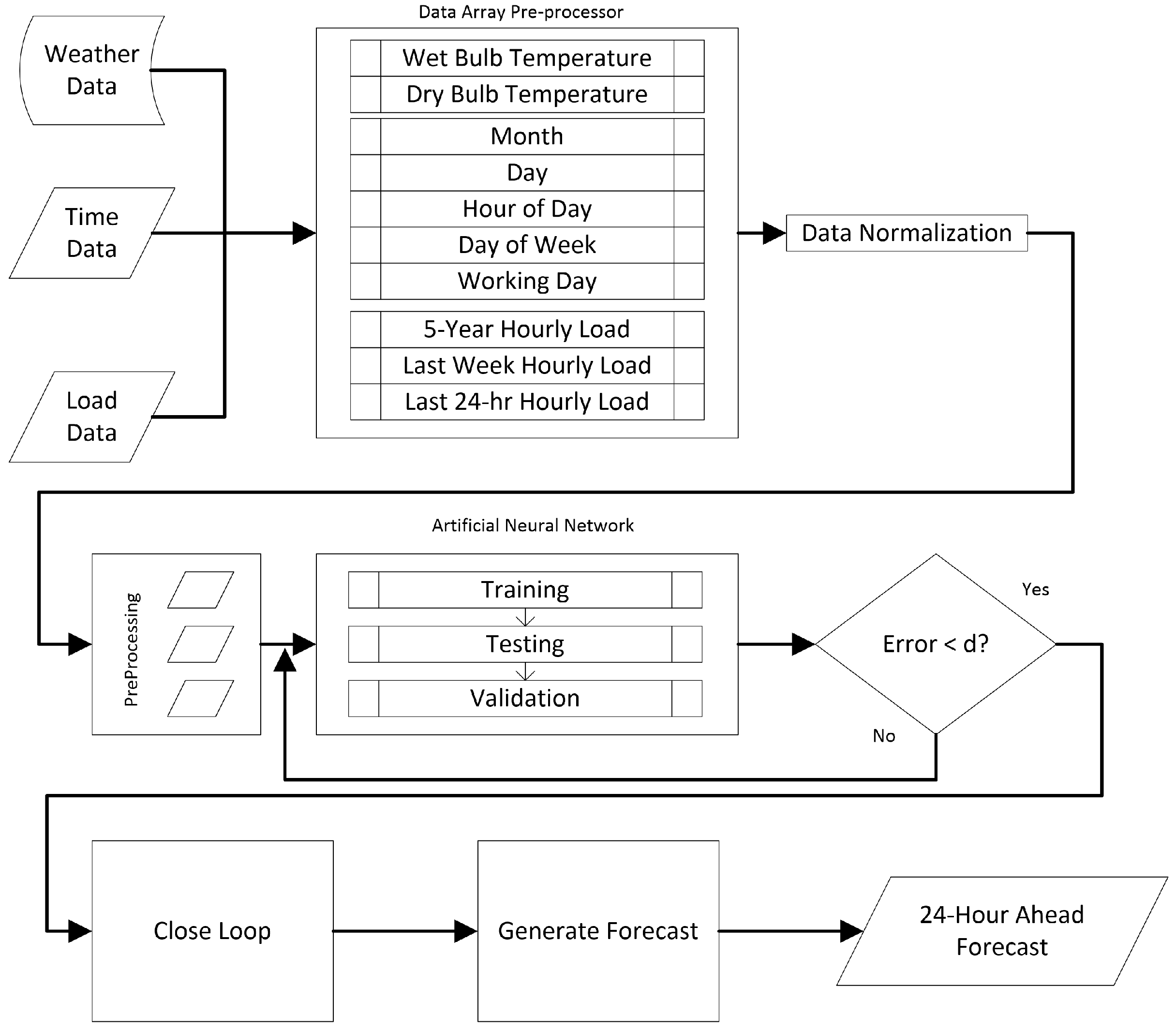
2. Proposed Framework
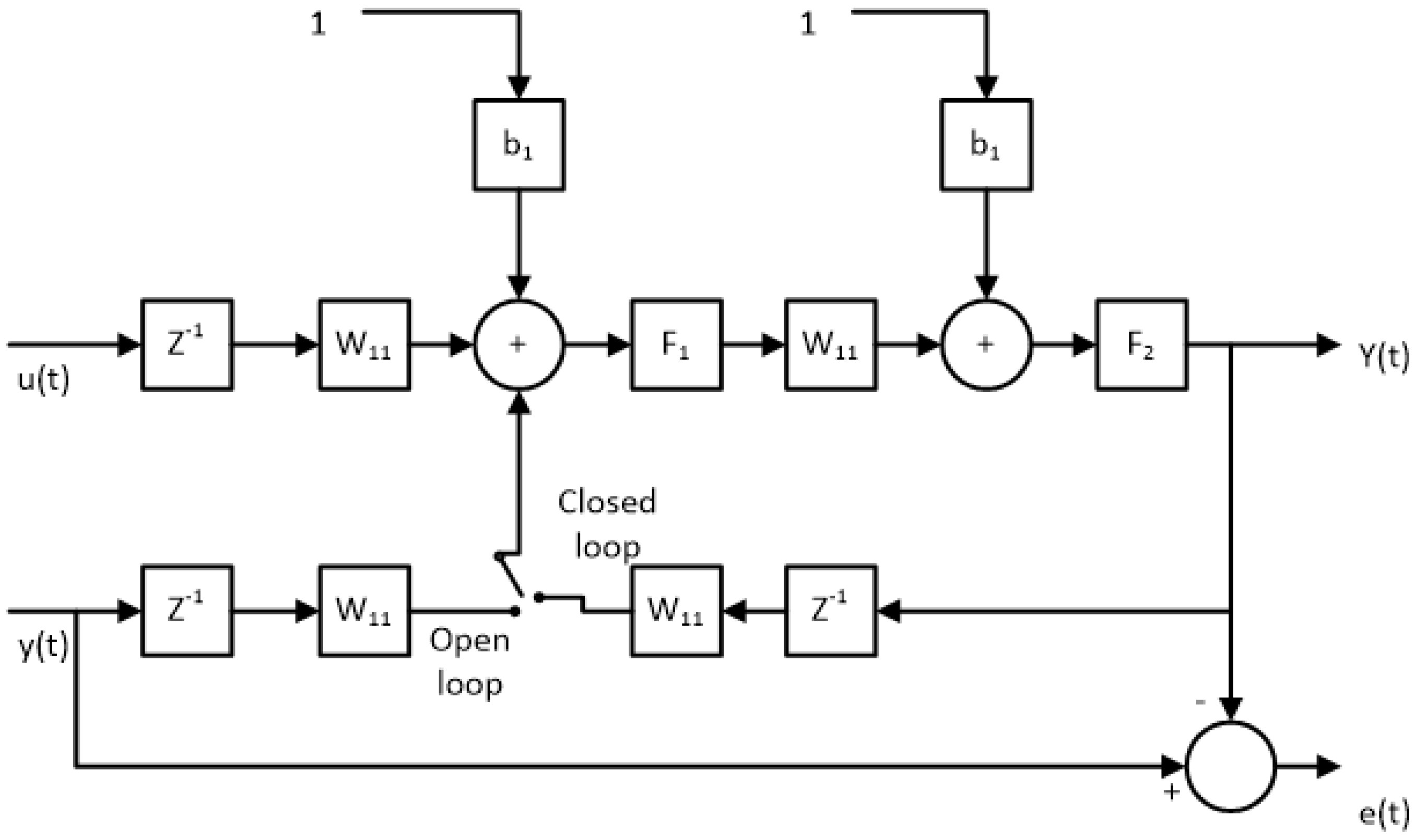
2.1. NARX Model
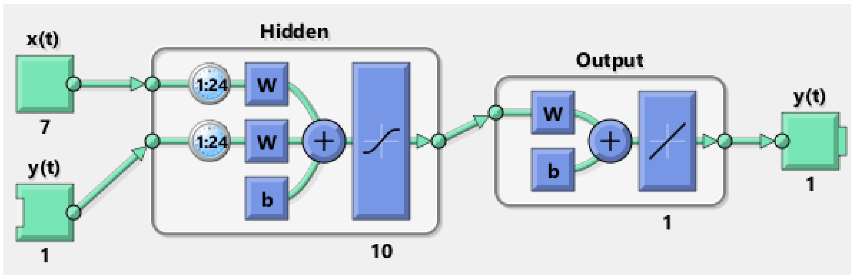
Neural Network Description
2.2. Simulation Environment
- Number of data groups: 10 different data periods were used;
- Number of neural networks: five different runs for each iteration in order to separate the outcome from the initial conditions;
- Number of neurons in the hidden layer: simulations were run from 5–30 neurons in increments of five.
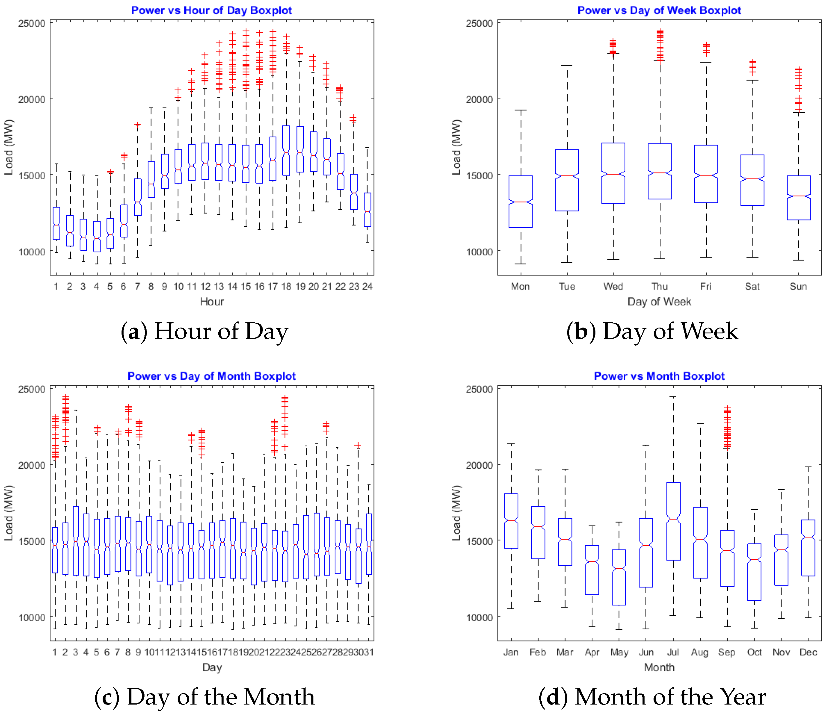
3. Data
4. Results
5. Discussion
- Different input periods (both in time and length): this is to include and exclude the effects of holidays, working and non-working days, seasons, etc. ANN NARX works well when sufficient cyclical data are available for training.
- The number of neurons in the hidden layer in the model: simulations were run from 1–30 neurons in the hidden layer. Typically, the forecast accuracy peaks at around 20 neurons.
- The number of delayed inputs and feedback: simulations ranging from 1 h–48 h delays were performed. A 24-hour time delay for inputs worked best.
- The redundancy on the input data: reinforcement of training data with the most recent available data. It was found that feeding redundant data for the last week and the last 24 h worked best.
Stability
6. Conclusions
Acknowledgments
Author Contributions
Conflicts of Interest
Abbreviations
| ANN | Artificial neural network |
| ARMA | Autoregressive and moving average model |
| ARMAX | Autoregressive and moving average with exogenous input model |
| CI | Computational intelligence |
| MAPE | Mean absolute percent error |
| NARX | Nonlinear autoregressive model with exogenous input |
| STLF | Short-term load forecasting |
References
- Satish, B.; Swarup, K.S.; Srinivas, S.; Rao, A.H. Effect of temperature on short term load forecasting using an integrated ANN. Electr. Power Syst. Res. 2004, 72, 95–101. [Google Scholar] [CrossRef]
- Nengling, T.; Stenzel, J.; Hongxiao, W. Techniques of applying wavelet transform into combined model for short-term load forecasting. Electr. Power Syst. Res. 2006, 76, 525–533. [Google Scholar] [CrossRef]
- Hippert, H.S.; Pedreira, C.E.; Souza, R.C. Neural networks for short-term load forecasting: A review and evaluation. IEEE Trans. Power Syst. 2001, 16, 44–55. [Google Scholar] [CrossRef]
- Hahn, H.; Meyer-Nieberg, S.; Pickl, S. Electric load forecasting methods: Tools for decision making. Eur. J. Oper. Res. 2009, 199, 902–907. [Google Scholar] [CrossRef]
- Metaxiotis, K.; Kagiannas, A.; Askounis, D.; Psarras, J. Artificial intelligence in short term electric load forecasting: A state-of-the-art survey for the researcher. Energy Convers. Manag. 2003, 44, 1525–1534. [Google Scholar] [CrossRef]
- Zhang, G.; Patuwo, E.B.; Hu, M.Y. Forecasting with artificial neural networks: The state of the art. Int. J. Forecast. 1998, 14, 35–62. [Google Scholar] [CrossRef]
- Tzafestas, S.; Tzafestas, E. Computational intelligence techniques for short-term electric load forecasting. J. Intell. Robot. Syst. Theory Appl. 2001, 31, 7–68. [Google Scholar] [CrossRef]
- Raza, M.; Khosravi, A. A review on artificial intelligence based load demand forecasting techniques for smart grid and buildings. Renew. Sustain. Energy Rev. 2015, 50, 1352–1372. [Google Scholar] [CrossRef]
- Ghayekhloo, M.; Menhaj, M.B.; Ghofrani, M. A hybrid short-term load forecasting with a new data preprocessing framework. Electr. Power Syst. Res. 2015, 119, 138–148. [Google Scholar] [CrossRef]
- Abdel-Aal, R.E. Univariate modeling and forecasting of monthly energy demand time series using abductive and neural networks. Comput. Ind. Eng. 2008, 54, 903–917. [Google Scholar] [CrossRef]
- Alfuhaid, A.S.; El-Sayed, M.A.; Mahmoud, M.S. Cascaded artificial neural networks for short-term load forecasting. IEEE Trans. Power Syst. 1997, 12, 1524–1529. [Google Scholar] [CrossRef]
- Bennett, C.; Stewart, R.A.; Lu, J. Autoregressive with exogenous variables and neural network short-term load forecast models for residential low voltage distribution networks. Energies 2014, 7, 2938–2960. [Google Scholar] [CrossRef]
- Bilgic, M.; Girep, C.; Aslanoglu, S.; Aydinalp-Koksal, M. Forecasting Turkey’s short term hourly load with artificial neural networks. In Proceedings of the 10th IET International Conference on Developments in Power System Protection (DPSP 2010), Managing the Change, Manchester, UK, 29 March–1 April 2010; pp. 1–5.
- Kandil, N.; Wamkeue, R.; Saad, M.; Georges, S. An efficient approach for short term load forecasting using artificial neural networks. Int. J. Electr. Power Energy Syst. 2006, 28, 525–530. [Google Scholar] [CrossRef]
- Bugwan, T.; King, R.T.A. Short term electrical load forecasting for mauritius using Artificial Neural Networks. In Proceedings of the IEEE International Conference on Systems, Man and Cybernetics, Singapore, 12–15 October 2008; pp. 3668–3673.
- Charytoniuk, W.; Chen, M.S. Very short-term load forecasting using artificial neural networks. IEEE Trans. Power Syst. 2000, 15, 263–268. [Google Scholar] [CrossRef]
- Ekonomou, L.; Oikonomou, D. Application and comparison of several artificial neural networks for forecasting the Hellenic daily electricity demand load. In Proceedings of the 7th WSEAS International Conference on Artificial Intelligence, Knowledge Engineering and Data Bases, Cairo, Egypt, 29–31 December 2008; pp. 67–71.
- Ekonomou, L.; Christodoulou, C.; Mladenov, V. A Short-Term Load Forecasting Method Using Artificial Neural Networks and Wavelet Analysis. Int. J. Power Syst. 2016, 1, 64–68. [Google Scholar]
- Gooi, H.; Teo, C.; Chin, L.; Ang, S.; Khor, E. Adaptive short-term load forecasting using artificial neural networks. In Proceedings of the 1993 IEEE Region 10 Conference on Computer, Communication, Control and Power Engineering (TENCON ’93), Beijing, China, 19–21 October 1993.
- Tee, C.Y.; Cardell, J.B.; Ellis, G.W. Short-term load forecasting using artificial neural networks. In Proceedings of the North American Power Symposium (NAPS), Starkville, MI, USA, 5–7 October 2009; pp. 1–6.
- Harun, M.H.H.; Othman, M.M.; Musirin, I. Short term load forecasting (STLF) using artificial neural network based multiple lags and stationary time series. In Proceedings of the 4th International Power Engineering and Optimization Conference, Shah Alam, Malaysia, 23–24 June 2010; pp. 363–370.
- Hernandez, L.; Baladron Zorita, C.; Aguiar Perez, J.M.; Carro Martinez, B.; Sanchez Esguevillas, A.; Lloret, J. Short-Term Load Forecasting for Microgrids Based on Artificial Neural Networks. Energies 2013, 6, 1385–1408. [Google Scholar] [CrossRef]
- Hernandez, L.; Baladron, C.; Aguiar, J.M.; Calavia, L.; Carro, B.; Sanchez-Esguevillas, A.; Sanjuan, J.; Gonzalez, L.; Lloret, J. Improved short-term load forecasting based on two-stage predictions with artificial neural networks in a microgrid environment. Energies 2013, 6, 4489–4507. [Google Scholar] [CrossRef]
- Kalaitzakis, K.; Stavrakakis, G.S.; Anagnostakis, E.M. Short-term load forecasting based on artificial neural networks parallel implementation. Electr. Power Syst. Res. 2002, 63, 185–196. [Google Scholar] [CrossRef]
- Khotanzad, A.; Afkhami-Rohani, R.; Lu, T.L.; Abaye, A.; Davis, M.; Maratukulam, D.J. ANNSTLF—A neural-network-based electric load forecasting system. IEEE Trans. Neural Netw. 1997, 8, 835. [Google Scholar] [CrossRef] [PubMed]
- Kiartzis, S.; Zoumas, C.; Bakirtzis, A.; Petridis, V. Data pre-processing for short-term load forecasting in an autonomous power system using artificial neural networks. In Proceedings of the Third IEEE International Conference on Electronics, Circuits, and Systems (ICECS’96), Rodos, Greece, 13–16 October 1996; Volume 2, pp. 1021–1024.
- Kiartzis, S.J.; Bakirtzis, A.G.; Petridis, V. Short-term load forecasting using neural networks. Electr. Power Syst. Res. 1995, 33, 1–6. [Google Scholar] [CrossRef]
- Matsumoto, T.; Kitamura, S.; Ueki, Y.; Matsui, T. Short-term load forecasting by artificial neural networks using individual and collective data of preceding years. In Proceedings of the Second International Forum on Applications of Neural Networks to Power Systems (ANNPS ’93), Yokohama, Japan, 19–22 April 1993; pp. 245–250.
- Moharari, N.S.; Debs, A.S. An artificial neural network based short term load forecasting with special tuning for weekends and seasonal changes. In Proceedings of the Second International Forum on Applications of Neural Networks to Power Systems (ANNPS’93), Yokohama, Japan, 19–22 April 1993; pp. 279–283.
- Papalexopoulos, A.; Hao, S.; Peng, T.M. Short-term system load forecasting using an artificial neural network. In Proceedings of the Second International Forum on Applications of Neural Networks to Power Systems (ANNPS’93), Yokohama, Japan, 19–22 April 1993; pp. 239–244.
- Reinschmidt, K.; Ling, B. Artificial neural networks in short term load forecasting. In Proceedings of the 4th IEEE Conference on Control Applications, Columbus, OH, USA, 28–29 September 1995; pp. 209–214.
- Santos, J.P.; Gomes, M.A.; Pires, A.J. Next hour load forecast in medium voltage electricity distribution. Int. J. Energy Sect. Manag. 2008, 2, 439–448. [Google Scholar] [CrossRef]
- Santos, P.J.; Martins, A.G.; Pires, A.J. On the use of reactive power as an endogenous variable in short-term load forecasting. Int. J. Energy Res. 2003, 27, 513–529. [Google Scholar] [CrossRef]
- Shimakura, Y.; Fujisawa, Y.; Maeda, Y.; Makino, R.; Kishi, Y.; Ono, M.; Fann, J.Y.; Fukusima, N. Short-term load forecasting using an artificial neural network. In Proceedings of the Second International Forum on Applications of Neural Networks to Power Systems (ANNPS ’93), Yokohama, Japan, 19–22 April 1993; pp. 233–238.
- Zhang, S.; Lian, J.; Zhao, Z.; Xu, H.; Liu, J. Grouping model application on artificial neural networks for short-term load forecasting. In Proceedings of the 7th World Congress on Intelligent Control and Automation (WCICA), Chongqing, China, 25–27 June 2008; pp. 6203–6206.
- Sinha, A. Short term load forecasting using artificial neural networks. In Proceedings of the IEEE International Conference on Industrial Technology, Goa, India, 19–22 January 2000; Volume 1, pp. 548–553.
- Da Silva, A.P.A.; Ferreira, V.H.; Velasquez, R.M.G. Input space to neural network based load forecasters. Int. J. Forecast. 2008, 24, 616–629. [Google Scholar] [CrossRef]
- Ferreira, V.H.; Alves da Silva, A.P. Toward estimating autonomous neural network-based electric load forecasters. IEEE Trans. Power Syst. 2007, 22, 1554–1562. [Google Scholar] [CrossRef]
- Santos, P.J.; Martins, A.G.; Pires, A.J. Designing the input vector to ANN-based models for short-term load forecast in electricity distribution systems. Int. J. Electr. Power Energy Syst. 2007, 29, 338–347. [Google Scholar] [CrossRef]
- Arahal, M.R.; Cepeda, A.; Camacho, F. Input variable Selection for Forcasting Models. In Proceedings of the 15th IFAC World Congress on Automatic Control, Barcelona, Spain, 21–26 July 2002.
- De Andrade, L.C.M.; Oleskovicz, M.; Santos, A.Q.; Coury, D.V.; Fernandes, R.A.S. Very short-term load forecasting based on NARX recurrent neural networks. In Proceedings of the IEEE PES General Meeting Conference and Exposition, National Harbor, MD, USA, 27–31 July 2014; pp. 1–5.
- Chen, H.; Du, Y.; Jiang, J.N. Weather sensitive short-term load forecasting using knowledge-based ARX models. In Proceedings of the IEEE Power Engineering Society General Meeting, San Francisco, CA, USA, 12–16 June 2005; Volume 1, pp. 190–196.
- Fattaheian, S.; Fereidunian, A.; Gholami, H.; Lesani, H. Hour-ahead demand forecasting in smart grid using support vector regression (SVR). Int. Trans. Electr. Energy Syst. 2014, 24, 1650–1663. [Google Scholar] [CrossRef]
- Hayati, M. Short term load forecasting using artificial neural networks for the west of Iran. J. Appl. Sci. 2007, 7, 1582–1588. [Google Scholar]
- Hernandez, L.; Baladron, C.; Aguiar, J.M.; Carro, B.; Sanchez-Esguevillas, A.; Lloret, J. Artificial neural networks for short-term load forecasting in microgrids environment. Energy 2014, 75, 252–264. [Google Scholar] [CrossRef]
- Hsu, Y.Y.; Yang, C.C. Design of artificial neural networks for short-term load forecasting. Part II. Multilayer feedforward networks for peak load and valley load forecasting. IEE Proc. C Gener. Transm. Distrib. 1991, 138, 414–418. [Google Scholar] [CrossRef]
- Hsu, Y.Y.; Yang, C.C. Design of artificial neural networks for short-term load forecasting. Part I. Self-organising feature maps for day type identification. IEE Proc. C Gener. Transm. Distrib. 1991, 138, 407–413. [Google Scholar] [CrossRef]
- Marin, F.J.; Garcia-Lagos, F.; Joya, G.; Sandoval, F. Global model for short-term load forecasting using artificial neural networks. IEE Proc. C Gener. Transm. Distrib. 2002, 149, 121–125. [Google Scholar] [CrossRef]
- Badri, A.; Ameli, Z.; Birjandi, A.M. Application of Artificial Neural Networks and Fuzzy logic Methods for Short Term Load Forecasting. Energy Procedia 2012, 14, 1883–1888. [Google Scholar] [CrossRef]
- Khosravi, A.; Nahavandi, S.; Creighton, D.; Srinivasan, D. Interval type-2 fuzzy logic systems for load forecasting: A comparative study. IEEE Trans. Power Syst. 2012, 27, 1274–1282. [Google Scholar] [CrossRef]
- Kim, K.H. Implementation of hybrid short-term load forecasting system using artificial neural networks and fuzzy expert systems. IEEE Trans. Power Syst. 1995, 10, 1534–1539. [Google Scholar]
- Mahmoud, T.S.; Habibi, D.; Hassan, M.Y.; Bass, O. Modelling self-optimised short term load forecasting for medium voltage loads using tunning fuzzy systems and Artificial Neural Networks. Energy Convers. Manag. 2015, 106, 1396–1408. [Google Scholar] [CrossRef]
- Santos, P.; Rafael, S.; Lobato, P.; Pires, A. A STLF in distribution systems—A short comparative study between ANFIS Neuro-Fuzzy and ANN approaches—Part I. In Proceedings of the International Conference on Power Engineering, Energy and Electrical Drives (POWERENG), Lisbon, Portugal, 18–20 March 2009; pp. 661–665.
- Rafael, S.; Santos, P.; Lobato, P.; Pires, A. A STLF in distribution systems—A short comparative study between ANFIS Neuro-Fuzzy and ANN approaches—Part II. In Proceedings of the International Conference on Power Engineering, Energy and Electrical Drives (POWERENG), Lisbon, Portugal, 18–20 March 2009.
- Srinivasan, D. Evolving artificial neural networks for short term load forecasting. Neurocomputing 1998, 23, 265–276. [Google Scholar] [CrossRef]
- Subbaraj, P.; Rajasekaran, V. Short Term Hourly Load Forecasting Using Combined Artificial Neural Networks. In Proceedings of the International Conference on Conference on Computational Intelligence and Multimedia Applications, Sivakasi, India, 13–15 December 2007; Volume 1, pp. 155–163.
- Sun, C.; Song, J.; Li, L.; Ju, P. Implementation of hybrid short-term load forecasting system with analysis of temperature sensitivities. Soft Comput. 2008, 12, 633–638. [Google Scholar] [CrossRef]
- Yang, H.T.; Huang, C.M. New short-term load forecasting approach using self-organizing fuzzy ARMAX models. IEEE Trans. Power Syst. 1998, 13, 217–225. [Google Scholar] [CrossRef]
- Carpinteiro, O.A.S.; Reis, A.J.R.; da Silva, A.P.A. A hierarchical neural model in short-term load forecasting. Appl. Soft Comput. 2004, 4, 405–412. [Google Scholar] [CrossRef]
- Crone, S.F.; Guajardo, J.; Weber, R. A study on the ability of support vector regression and neural networks to forecast basic time series patterns. In Proceedings of the 4th IFIP International Conference on Artificial Intelligence in Theory and Practice, Perth, Australia, 6–7 October 2006; pp. 149–158.
- Buitrago, J.; Abdulaal, A.; Asfour, S. Electric load pattern classification using parameter estimation, clustering and artificial neural networks. Int. J. Power Energy Syst. 2015, 35, 167–174. [Google Scholar] [CrossRef]
- Abdulaal, A.; Buitrago, J.; Asfour, S. Electric Load Pattern Classification for Demand-side Management Planning: A Hybrid Approach. In Software Engineering and Applications: Advances in Power and Energy Systems; Press, A., Ed.; ACTA Press: Marina del Rey, CA, USA, 2015. [Google Scholar]
- Lopez, M.; Valero, S.; Senabre, C.; Aparicio, J.; Gabaldon, A. Application of SOM neural networks to short-term load forecasting: The Spanish electricity market case study. Electr. Power Syst. Res. 2012, 91, 18–27. [Google Scholar] [CrossRef]
- Liang, R.H.; Hsu, Y.Y. A hybrid artificial neural network—Differential dynamic programming approach for short-term hydro scheduling. Electr. Power Syst. Res. 1995, 33, 77–86. [Google Scholar] [CrossRef]
- Venturini, M. Simulation of compressor transient behavior through recurrent neural network models. J. Turbomach. Trans. ASME 2006, 128, 444–454. [Google Scholar] [CrossRef]
- England, I.N. Energy, Load and Demand Reports; ISO New England: Holyoke, MA, USA, 2015. [Google Scholar]
- Irigoyen, E.; Pinzolas, M. Numerical bounds to assure initial local stability of NARX multilayer perceptrons and radial basis functions. Neurocomputing 2008, 72, 539–547. [Google Scholar] [CrossRef]

| Exogenous | Endogenous | Time Lag |
|---|---|---|
| Month | Load | Last 24 h |
| Day | ||
| Hour of Day | ||
| Day of Week | ||
| Working Day | ||
| Wet Bulb Temperature | ||
| Dew Point |
| ANN Architecture | |
|---|---|
| Input Nodes | One node for each input variable |
| Hidden Layers | 1 |
| Hidden Nodes | Equal to number of input nodes |
| Output Nodes | Equal to size of forecasting horizon (1 node) |
| Interconnection | Full |
| Activation Function | Sigmoid Function
|
| Learning Algorithm | Levenberg–Marquardt backpropagation |
| FitNet | ARMAX | State Space | NARXNet | ||||||
|---|---|---|---|---|---|---|---|---|---|
| Hour | Actual | Forecast | AE% | Forecast | AE% | Forecast | AE% | Forecast | AE% |
| 1 | 12,115 | 12,165 | 0.41 | 12,248 | 1.1 | 12,269 | 1.27 | 12,141 | 0.21 |
| 2 | 11,576 | 11,713 | 1.19 | 11,749 | 1.49 | 11,553 | 0.2 | 11,657 | 0.7 |
| 3 | 11,254 | 11,349 | 0.85 | 11,278 | 0.21 | 10,679 | 5.11 | 11,155 | 0.88 |
| 4 | 11,073 | 11,074 | 0.01 | 10,933 | 1.26 | 10,090 | 8.87 | 11,229 | 1.41 |
| 5 | 11,084 | 10,963 | 1.09 | 10,886 | 1.79 | 10,901 | 1.65 | 11,134 | 0.45 |
| 6 | 11,326 | 11,123 | 1.79 | 11,191 | 1.19 | 11,246 | 0.7 | 11,449 | 1.08 |
| 7 | 11,780 | 11,649 | 1.11 | 11,624 | 1.32 | 12,067 | 2.44 | 11,790 | 0.09 |
| 8 | 12,338 | 12,456 | 0.96 | 12,054 | 2.3 | 13,132 | 6.44 | 12,270 | 0.55 |
| 9 | 13,193 | 13,402 | 1.59 | 12,932 | 1.98 | 13,532 | 2.57 | 12,960 | 1.77 |
| 10 | 13,752 | 13,757 | 0.04 | 13,694 | 0.42 | 13,452 | 2.18 | 13,790 | 0.28 |
| 11 | 13,978 | 13,894 | 0.6 | 14,023 | 0.32 | 13,502 | 3.41 | 13,997 | 0.14 |
| 12 | 14,018 | 13,867 | 1.07 | 14,077 | 0.42 | 13,825 | 1.38 | 14,022 | 0.03 |
| 13 | 13,980 | 13,708 | 1.94 | 14,076 | 0.69 | 14,098 | 0.85 | 14,052 | 0.52 |
| 14 | 13,900 | 13,660 | 1.73 | 14,041 | 1.02 | 14,141 | 1.74 | 13,842 | 0.42 |
| 15 | 13,905 | 13,777 | 0.92 | 14,051 | 1.05 | 14,260 | 2.55 | 13,928 | 0.16 |
| 16 | 14,298 | 14,053 | 1.71 | 14,554 | 1.79 | 14,782 | 3.38 | 14,153 | 1.01 |
| 17 | 15,634 | 14,726 | 5.81 | 15,916 | 1.8 | 15,509 | 0.8 | 15,452 | 1.16 |
| 18 | 16,275 | 15,280 | 6.11 | 16,452 | 1.09 | 15,931 | 2.11 | 16,725 | 2.77 |
| 19 | 16,144 | 15,500 | 3.99 | 16,257 | 0.7 | 15,855 | 1.79 | 15,935 | 1.3 |
| 20 | 15,633 | 15,412 | 1.41 | 15,769 | 0.87 | 15,506 | 0.81 | 15,872 | 1.53 |
| 21 | 15,020 | 14,879 | 0.94 | 15,227 | 1.38 | 15,048 | 0.19 | 15,241 | 1.47 |
| 22 | 13,927 | 13,974 | 0.34 | 14,069 | 1.02 | 14,319 | 2.81 | 14,141 | 1.54 |
| 23 | 12,656 | 12,811 | 1.22 | 12,679 | 0.18 | 13,179 | 4.13 | 12,573 | 0.66 |
| 24 | 11,509 | 11,553 | 0.38 | 11,584 | 0.65 | 11,885 | 3.27 | 11,546 | 0.32 |
| Maximum | 6.11 | 2.30 | 8.87 | 2.77 | |||||
| MAPE% | 1.55 | 1.09 | 2.53 | 0.85 | |||||
© 2017 by the authors; licensee MDPI, Basel, Switzerland. This article is an open access article distributed under the terms and conditions of the Creative Commons Attribution (CC-BY) license (http://creativecommons.org/licenses/by/4.0/).
Share and Cite
Buitrago, J.; Asfour, S. Short-Term Forecasting of Electric Loads Using Nonlinear Autoregressive Artificial Neural Networks with Exogenous Vector Inputs. Energies 2017, 10, 40. https://doi.org/10.3390/en10010040
Buitrago J, Asfour S. Short-Term Forecasting of Electric Loads Using Nonlinear Autoregressive Artificial Neural Networks with Exogenous Vector Inputs. Energies. 2017; 10(1):40. https://doi.org/10.3390/en10010040
Chicago/Turabian StyleBuitrago, Jaime, and Shihab Asfour. 2017. "Short-Term Forecasting of Electric Loads Using Nonlinear Autoregressive Artificial Neural Networks with Exogenous Vector Inputs" Energies 10, no. 1: 40. https://doi.org/10.3390/en10010040
APA StyleBuitrago, J., & Asfour, S. (2017). Short-Term Forecasting of Electric Loads Using Nonlinear Autoregressive Artificial Neural Networks with Exogenous Vector Inputs. Energies, 10(1), 40. https://doi.org/10.3390/en10010040