
A Unit Half-Logistic Geometric Distribution and Its Application in Insurance


Abstract
1. Introduction
2. Unit Half Logistic-Geometry Distribution
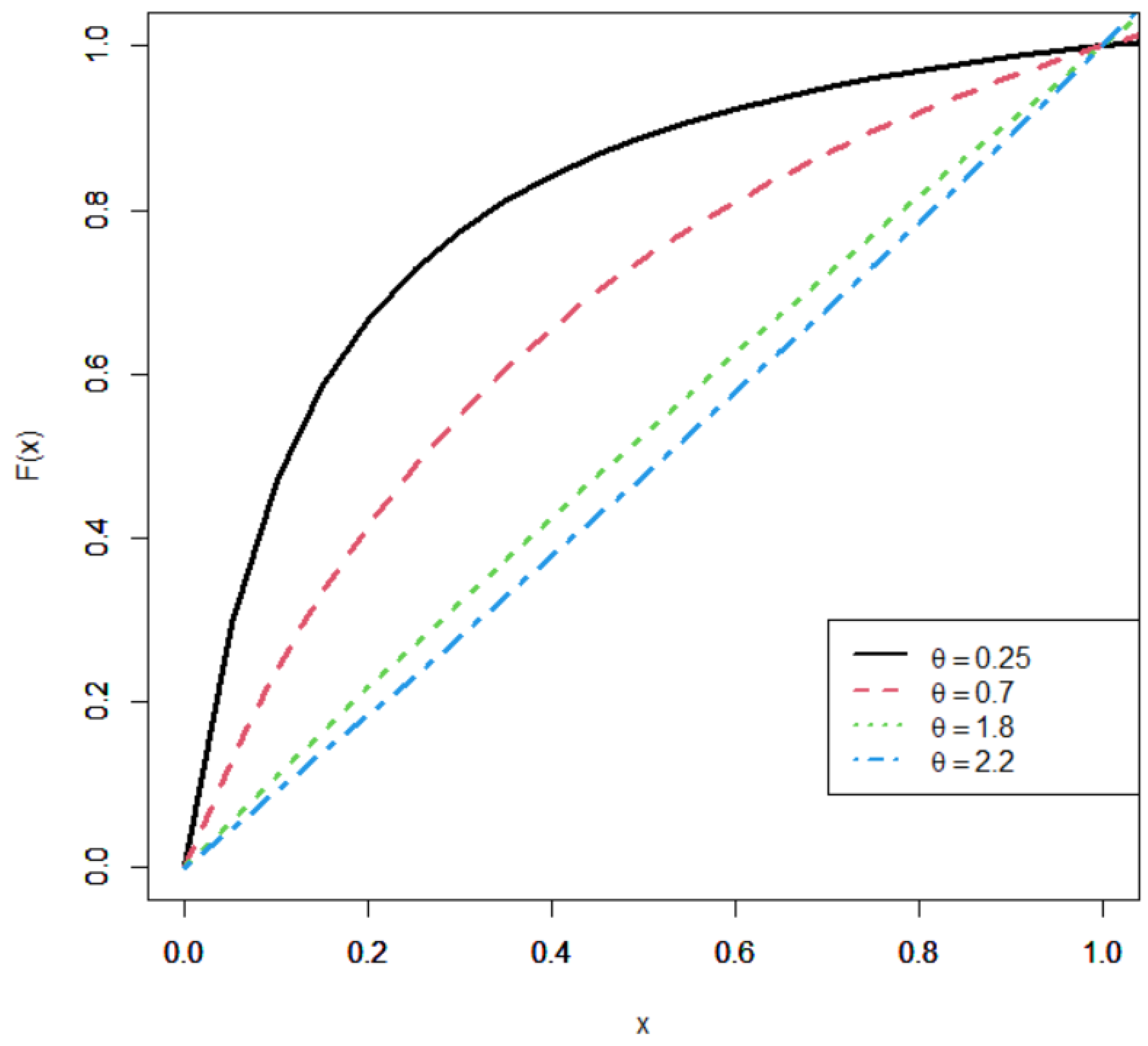
2.1. Cumulative and Density Functions of UHLG Distribution
- (i)
- decreasing function if ,
- (ii)
- increasing function if ,
- (iii)
- constant when .
- (i)
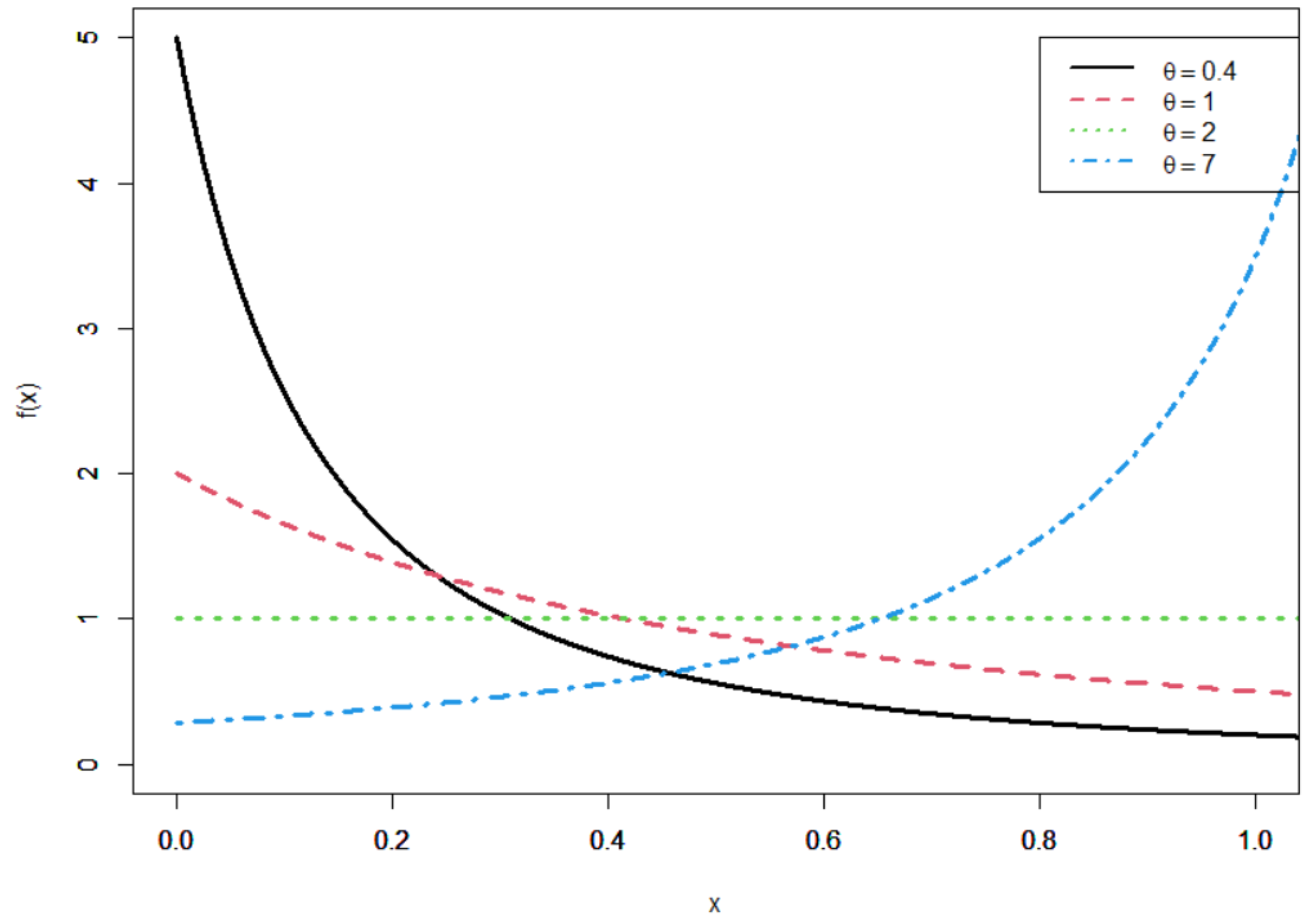
- When , the first derivative is negative, which implies that the pdf of the UHLG distribution is decreasing;
- (ii)
- When , the first derivative is positive, which implies that the pdf of the UHLG distribution is increasing;
- (iii)
- Lastly, when , the pdf of the UHLG distribution is constant and equal to 1. □
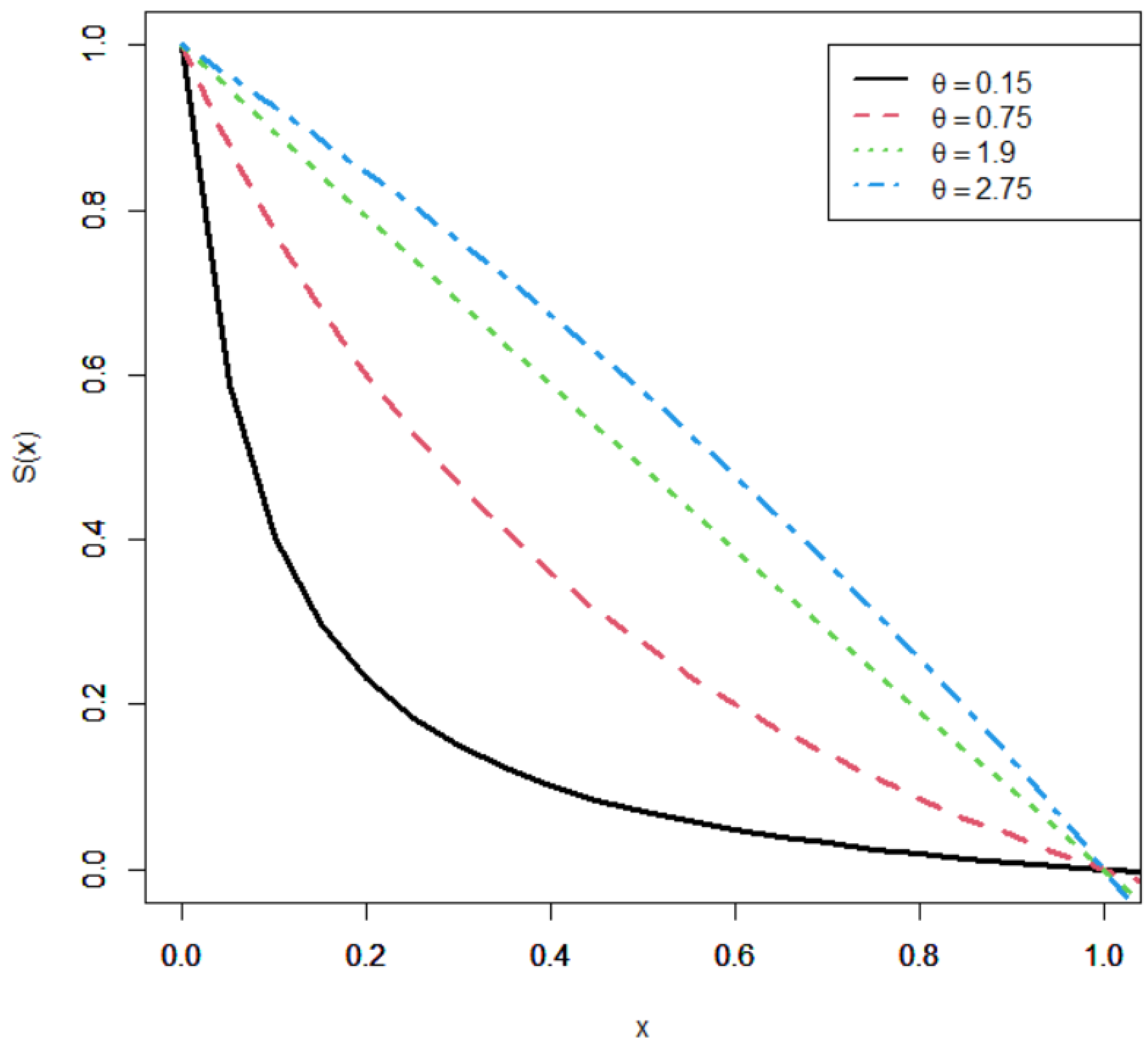
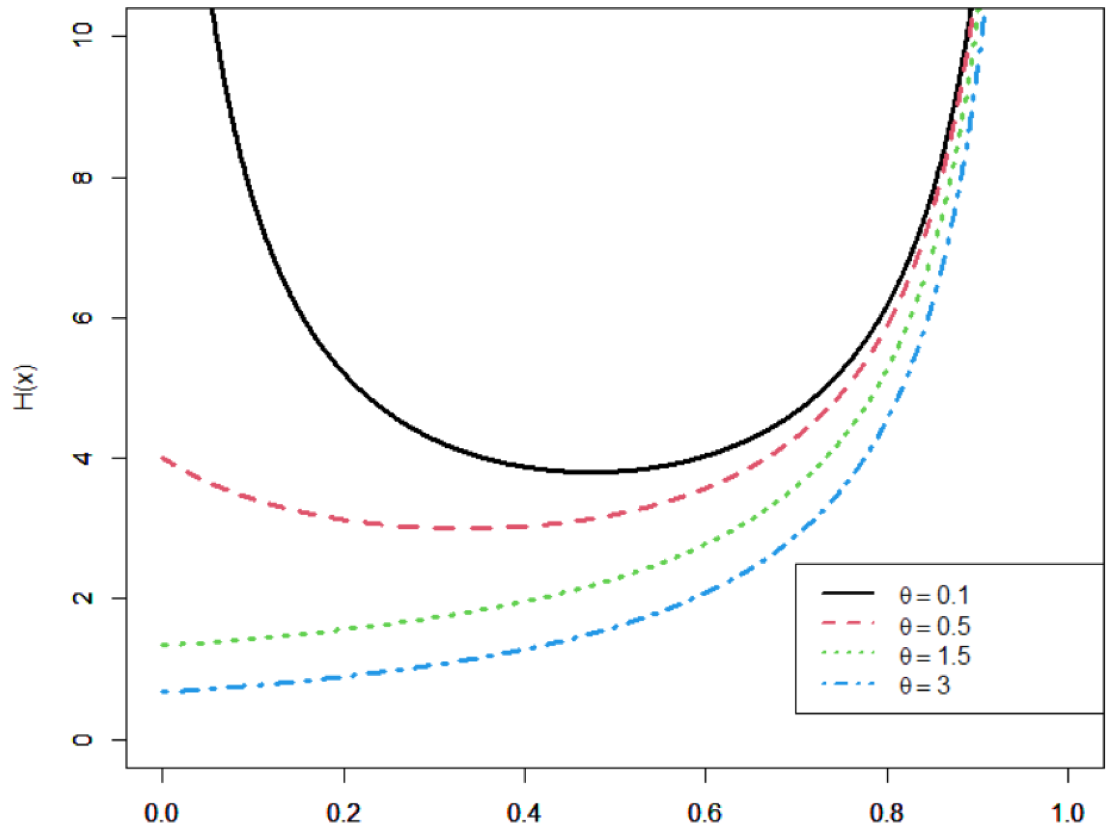
2.2. Survival and Hazard Functions of the UHLG Distribution
- (i)
- bathtub (U-shaped) function if ,
- (ii)
- increasing function if .
- (i)
- When , the sign of changes from negative to positive, which implies that the function is decreasing first and increasing second (bathtub shape) with minimum value equal to ;
- (ii)
- When , the sign of is always positive, which implies that the function is increasing.
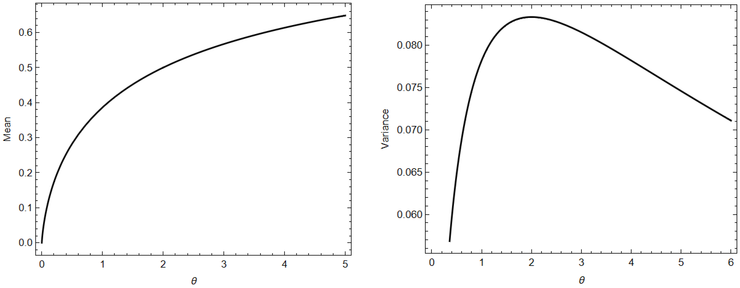
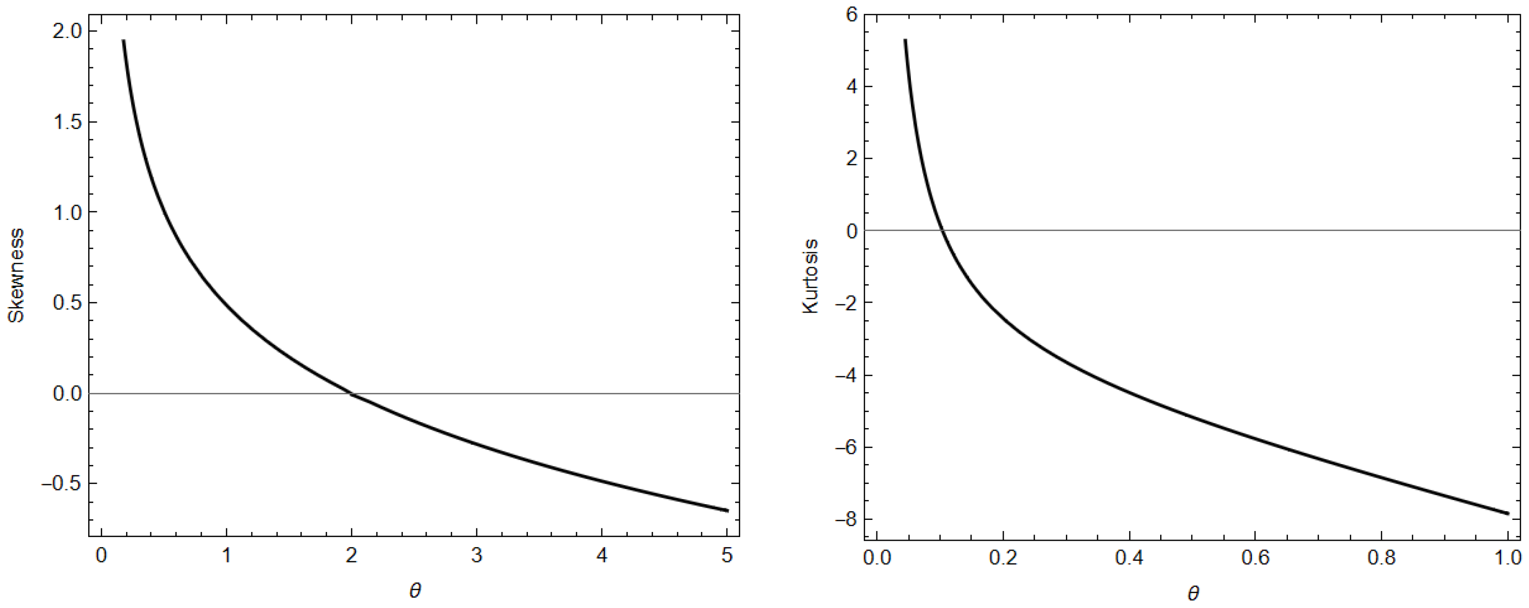
2.3. Moments
2.4. Incomplete Moments and Related Measures
2.5. Stress Strength Parameter
2.6. Stochastic Ordering
3. Parameter Estimation
3.1. Maximum Likelihood Estimation Method (MLE)
3.2. Bayesian Estimation Method
- Step 1: Start with an arbitrary initial value where and set .
- Step 2: Generate a proposal from normal distribution, i.e., .
- Step 3: Calculate the acceptance probability function
- Step 4: Generate .
- Step 5: If put ; otherwise put .
- Step 6: Repeat steps (2) and (5) N times to have .
3.3. Cramer-Von-Mises Method
3.4. Least Squares Method
3.5. Method of Moments
3.6. Weighted Least Squares Method
4. Simulation Study
- ME converges to when the sample size, n, increases;
- AB tends to zero when the sample size, n, increases;
- MSE decreases when the sample size, n, increases;
- In general, MLE and BE methods are the best estimation methods compared with the previous methods.
5. Unit Half Logistic-Geometry Quantile Regression Model
5.1. Maximum Likelihood Estimates Method
5.2. Residual Analysis
6. Application
Risk Survey Data
- Firm cost (y) is the mean variable and represents the cost of the firm’s cost management effectiveness;
- Assume () represents the firm’s retention strategy;
- Cap () represents the indicator with value 1 if the firm uses a captive insurer and the value 0 otherwise;
- Sizelog () represents the log of firm’s size;
- Indcost () represents the risk in the firm’s industry;
- Central () represents the strategy of the firm’s centralization;
- Analy () represents the degree of importance of using analytical tools.
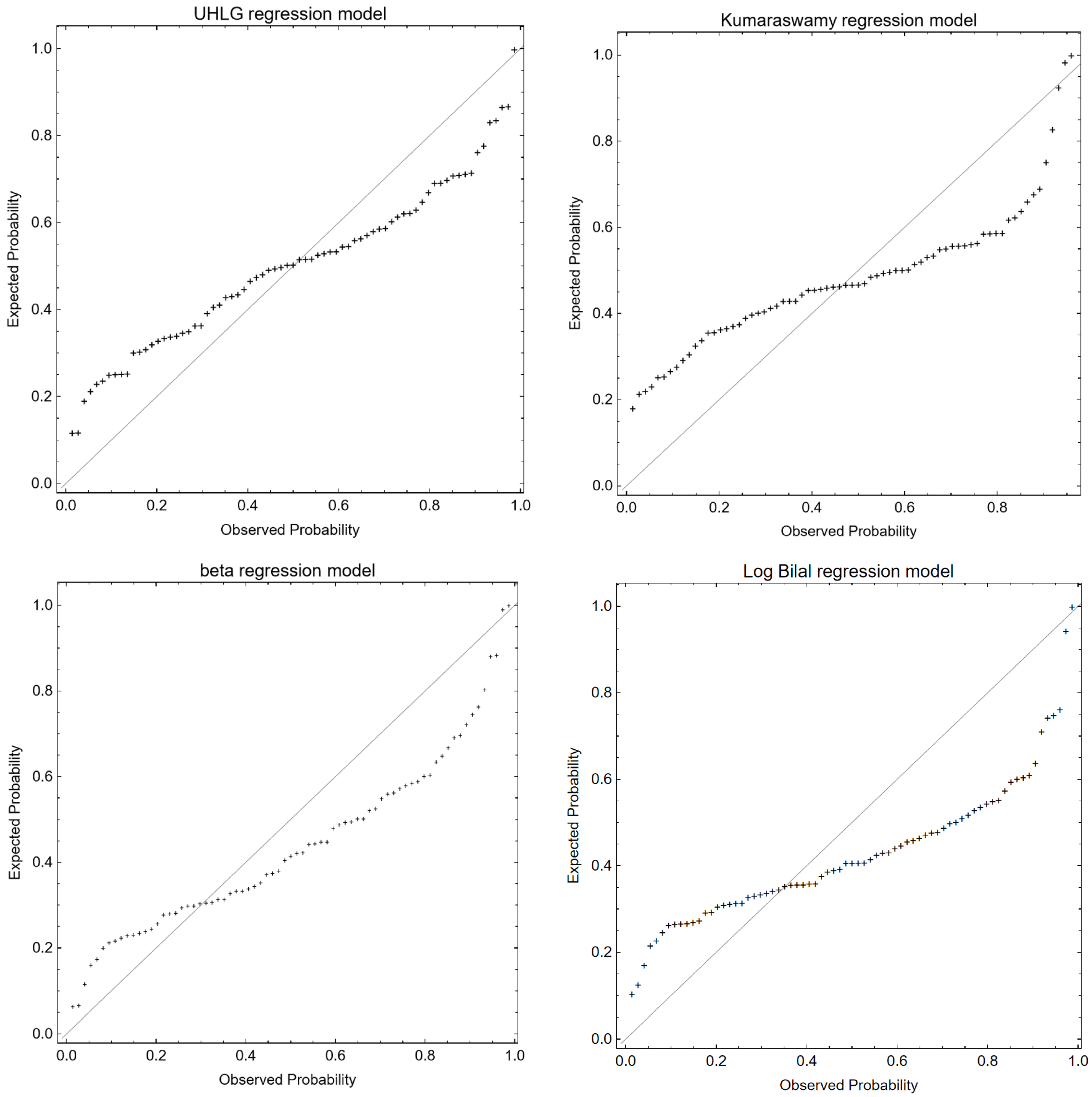
- All covariates have an impact on the firm’s cost management effectiveness;
- The UHLG regression model explains the greatest difference by using fewer parameters (-AIC = 192.34 and -BIC = 176.31);
- UHLG regression model gives the best fit to the data compared to the other models.
7. Conclusions
Author Contributions
Funding
Data Availability Statement
Conflicts of Interest
References
- Ramadan, A.T.; Tolba, A.H.; El-Desouky, B.S. Generalized power Akshaya distribution and its applications. Open J. Model. Simul. 2021, 4, 323–338. [Google Scholar] [CrossRef]
- El-Sagheer, R.M.; Tolba, A.H.; Jawa, T.M.; Sayed-Ahmed, N. Inferences for Stress-Strength Reliability Model in the Presence of Partially Accelerated Life Test to Its Strength Variable. Comput. Intell. Neurosci. 2022, 5, 4710536. [Google Scholar] [CrossRef] [PubMed]
- Abd El-Monsef, M.M.E.; El-Awady, M.M.; Seyam, M.M. A new quantile regression model for modelling child mortality. Int. J. Biomath. 2022, 10, 142–149. [Google Scholar]
- Altun, E.; Cordeiro, G.M. The unit-improved second-degree Lindley distribution: Inference and regression modelling. Comput. Stat. 2020, 35, 259–279. [Google Scholar] [CrossRef]
- Altun, E.; El-Morshedy, M.; Eliwa, M.S. A new regression model for bounded response variable: An alternative to the beta and unit-Lindley regression models. PLoS ONE 2021, 16, e0245627. [Google Scholar] [CrossRef] [PubMed]
- Bayes, C.L.; Bazán, J.L.; De Castro, M. A quantile parametric mixed regression model for bounded response variables. Stat. Its Interface 2017, 10, 483–493. [Google Scholar] [CrossRef]
- Cordeiro, G.M.; Silva, R.B.; Nascimento, A.D.C. Recent Advances in Lifetime and Reliability Models; Bentham Science Publishers: Oak Park, IL, USA, 2020; Volume 17, pp. 93–112. [Google Scholar]
- Ferrari, S.; Cribari-Neto, F. Beta regression for modelling rates and proportions. J. Appl. Stat. 2004, 31, 799–815. [Google Scholar] [CrossRef]
- Kumaraswamy, P. A generalized probability density function for double-bounded random processes. J. Hydrol. 1980, 46, 79–88. [Google Scholar] [CrossRef]
- Mitnik, P.A.; Baek, S. The Kumaraswamy distribution: Median-dispersion re-parameterizations for regression modelling and simulation-based estimation. Stat. Pap. 2013, 54, 177–192. [Google Scholar] [CrossRef]
- Gómez-Déniz, E.; Sordo, M.A.; Calderín-Ojeda, E. The Log-Lindley distribution as an alternative to the beta regression model with applications in insurance. Insur. Math. Econ. 2014, 54, 49–57. [Google Scholar] [CrossRef]
- Korkmaz, M.Ç.; Chesneau, C. On the unit Burr-XII distribution with the quantile regression modelling and applications. Comput. Appl. Math. 2021, 40, 1–26. [Google Scholar] [CrossRef]
- Mazucheli, J.; Menezes, A.F.B.; Ghitany, M.E. The unit-Weibull distribution and associated inference. J. Appl. Probab. Stat. 2018, 13, 1–22. [Google Scholar]
- Mazucheli, J.; Menezes, A.F.B.; Fernandes, L.B.; De Oliveira, R.P.; Ghitany, M.E. The unit-Weibull distribution as an alternative to the Kumaraswamy distribution for the modelling of quantiles conditional on covariates. J. Appl. Stat. 2020, 47, 954–974. [Google Scholar] [CrossRef] [PubMed]
- Muse, A.H.; Tolba, A.H.; Fayad, E.; Ali, O.A.A.; Nagy, M.; Yusuf, M. Modelling the COVID-19 mortality rate with a new versatile modification of the log-logistic distribution. Comput. Intell. Neurosci. 2021, 26, 203–224. [Google Scholar] [CrossRef] [PubMed]
- Mahmood, Z.; Jawa, M.T.; Sayed-Ahmed, N.; Khalil, E.M.; Muse, A.H.; Tolba, A.H. An Extended Cosine Generalized Family of Distributions for Reliability Modelling: Characteristics and Applications with Simulation Study. Math. Probl. Eng. 2022, 3, 112–128. [Google Scholar]
- Mazucheli, J.; Menezes, A.F.B.; Chakraborty, S. On the one parameter unit-Lindley distribution and its associated regression model for proportion data. J. Appl. Stat. 2019, 46, 700–714. [Google Scholar] [CrossRef]
- Mousa, A.M.; El-Sheikh, A.A.; Abdel-Fattah, M.A. A gamma regression for bounded continuous variables. Adv. Appl. Stat. 2016, 49, 305–321. [Google Scholar] [CrossRef]
- Sarhan, A.M.; El-Gohary, A.I.; Mustafa, A.; Tolba, A.H. Statistical analysis of regression competing risks model with covariates using Weibull sub-distributions. Int. J. Reliab. Appl. 2019, 2, 73–88. [Google Scholar]
- Sarhan, A.M.; El-Gohary, A.I.; Tolba, A.H. Statistical Analysis of a Competing Risks Model with Weibull Sub-Distributions. Appl. Math. 2017, 11, 1671–1690. [Google Scholar] [CrossRef][Green Version]
- Tadikamalla, P.R. On a family of distributions obtained by the transformation of the gamma distribution. J. Stat. Comput. Simul. 1981, 13, 209–214. [Google Scholar] [CrossRef]
- Liu, K.; Balakrishnan, N. Recurrence relations for moments of order statistics from half logistic-geometric distribution and their applications. Commun. Stat.-Simul. Comput. 2020, 17, 1–19. [Google Scholar] [CrossRef]
- Gradshteyn, I.S.; Ryzhik, I.M. Table of Integrals, Series, and Products; Academic Press: Cambridge, MA, USA, 2014; Volume 11. [Google Scholar]
- Mohamed, R.A.H.; Tolba, A.H.; Almetwally, E.M.; Ramadan, D.A. Inference of Reliability Analysis for Type II Half Logistic Weibull Distribution with Application of Bladder Cancer. Axioms 2022, 8, 386. Available online: https://www.mdpi.com/2075-1680/11/8/386 (accessed on 6 August 2022). [CrossRef]
- Shanmugam, R. The Stress-Strength Model and Its Generalizations: Theory and Applications; Taylor & Francis: Boca Raton, FL, USA, 2004; Volume 16, pp. 84–105. [Google Scholar]
- Frank, W.J.O. NIST Handbook of Mathematical Functions; Cambridge University Press: Cambridge, UK, 2010; Volume 17, pp. 224–251. [Google Scholar]
- Balakrishnan, N. Order statistics from the half logistic distribution. J. Stat. Comput. Simul. 1985, 20, 287–309. [Google Scholar] [CrossRef]
- Belzunce, F.; Riquelme, C.M.; Mulero, J. An Introduction to Stochastic Orders; Academic Press: Cambridge, MA, USA, 2015; Volume 12, pp. 165–187. [Google Scholar]
- Abushal, T.A.; Kumar, J.; Muse, A.H.; Tolba, A.H. Estimation for Akshaya Failure Model with Competing Risks under Progressive Censoring Scheme with Analyzing of Thymic Lymphoma of Mice Application. Complexity 2022, 2022, 5151274. [Google Scholar] [CrossRef]
- McCool, J.I. Using the Weibull Distribution: Reliability, Modelling and Inference; John Wiley & Sons: Hoboken, NJ, USA, 2012; Volume 950, pp. 43–66. [Google Scholar]
- Zhang, P.; Qiu, Z.; Shi, C. Simplexreg: An R package for regression analysis of proportional data using the simplex distribution. J. Stat. Softw. 2016, 71, 51–76. [Google Scholar] [CrossRef]
- Nurunnabi, A.A.M.; Hadi, A.S.; Imon, A.H.M.R. Procedures for the identification of multiple influential observations in linear regression. J. Appl. Stat. 2014, 41, 1315–1331. [Google Scholar] [CrossRef]
- Cox, D.R.; Snell, E.J. A general definition of residuals. J. R. Stat. Soc. Ser. B Methodol. 1968, 30, 248–265. [Google Scholar] [CrossRef]
- Dunn, P.K.; Smyth, G.K. Randomized quantile residuals. J. Comput. Graph. Stat. 1996, 5, 121–143. [Google Scholar]


| n | CVMEs | |||||||||
|---|---|---|---|---|---|---|---|---|---|---|
| ME | AB | MSE | ME | AB | MSE | ME | AB | MSE | ||
| 20 | 0.115 | 0.015 | 0.002 | 0.109 | 0.009 | 0.004 | 0.148 | 0.049 | 0.058 | |
| 70 | 0.103 | 0.003 | 0.001 | 0.106 | 0.006 | 0.001 | 0.150 | 0.050 | 0.048 | |
| 100 | 0.102 | 0.002 | 0.001 | 0.101 | 0.001 | 0.000 | 0.147 | 0.047 | 0.046 | |
| 150 | 0.101 | 0.001 | 0.001 | 0.102 | 0.002 | 0.000 | 0.162 | 0.062 | 0.042 | |
| 200 | 0.101 | 0.001 | 0.001 | 0.103 | 0.003 | 0.000 | 0.150 | 0.050 | 0.036 | |
| 20 | 0.573 | 0.073 | 0.052 | 0.539 | 0.039 | 0.065 | 0.535 | 0.035 | 0.075 | |
| 70 | 0.516 | 0.016 | 0.011 | 0.532 | 0.032 | 0.020 | 0.549 | 0.049 | 0.065 | |
| 100 | 0.509 | 0.009 | 0.008 | 0.507 | 0.007 | 0.009 | 0.525 | 0.025 | 0.051 | |
| 150 | 0.503 | 0.003 | 0.005 | 0.509 | 0.009 | 0.007 | 0.531 | 0.031 | 0.044 | |
| 200 | 0.504 | 0.004 | 0.004 | 0.515 | 0.015 | 0.006 | 0.543 | 0.043 | 0.034 | |
| 20 | 1.031 | 0.131 | 0.168 | 0.967 | 0.067 | 0.215 | 0.911 | 0.011 | 0.096 | |
| 70 | 0.929 | 0.029 | 0.037 | 0.951 | 0.051 | 0.067 | 0.932 | 0.032 | 0.087 | |
| 100 | 0.916 | 0.016 | 0.026 | 0.911 | 0.011 | 0.035 | 0.927 | 0.027 | 0.074 | |
| 150 | 0.905 | 0.005 | 0.016 | 0.914 | 0.014 | 0.027 | 0.942 | 0.042 | 0.062 | |
| 200 | 0.907 | 0.007 | 0.013 | 0.924 | 0.024 | 0.019 | 0.922 | 0.022 | 0.055 | |
| n | LSEs | MMEs | WLSEs | |||||||
|---|---|---|---|---|---|---|---|---|---|---|
| ME | AB | MSE | ME | AB | MSE | ME | AB | MSE | ||
| 20 | 0.149 | 0.049 | 0.107 | 0.294 | 0.194 | 0.352 | 0.144 | 0.044 | 0.116 | |
| 70 | 0.155 | 0.055 | 0.088 | 0.295 | 0.195 | 0.327 | 0.146 | 0.046 | 0.089 | |
| 100 | 0.163 | 0.063 | 0.076 | 0.256 | 0.156 | 0.297 | 0.161 | 0.061 | 0.089 | |
| 150 | 0.151 | 0.051 | 0.069 | 0.245 | 0.145 | 0.237 | 0.161 | 0.061 | 0.066 | |
| 200 | 0.150 | 0.050 | 0.053 | 0.271 | 0.171 | 0.211 | 0.161 | 0.061 | 0.042 | |
| 20 | 0.524 | 0.024 | 0.074 | 0.979 | 0.479 | 1.724 | 0.625 | 0.125 | 0.312 | |
| 70 | 0.538 | 0.038 | 0.067 | 0.890 | 0.390 | 1.702 | 0.616 | 0.116 | 0.302 | |
| 100 | 0.537 | 0.037 | 0.061 | 0.938 | 0.438 | 1.664 | 0.625 | 0.125 | 0.291 | |
| 150 | 0.540 | 0.040 | 0.059 | 0.859 | 0.359 | 1.568 | 0.621 | 0.121 | 0.285 | |
| 200 | 0.542 | 0.042 | 0.056 | 0.915 | 0.415 | 1.497 | 0.614 | 0.114 | 0.264 | |
| 20 | 0.909 | 0.009 | 0.083 | 1.225 | 0.325 | 2.049 | 1.065 | 0.165 | 0.608 | |
| 70 | 0.930 | 0.030 | 0.082 | 1.131 | 0.231 | 2.049 | 1.084 | 0.184 | 0.582 | |
| 100 | 0.920 | 0.020 | 0.079 | 1.164 | 0.264 | 1.962 | 1.064 | 0.164 | 0.571 | |
| 150 | 0.935 | 0.035 | 0.074 | 1.098 | 0.198 | 1.924 | 1.080 | 0.180 | 0.554 | |
| 200 | 0.900 | 0.000 | 0.063 | 1.085 | 0.185 | 1.852 | 1.084 | 0.184 | 0.521 | |
| Model | AIC | AICC | BIC | K-S | p-Value | ||
|---|---|---|---|---|---|---|---|
| unit half logistic | 0.132 | - | −177.02 | −177.01 | −174.78 | 0.1191 | 0.2515 |
| log Bilal | 3.464 | - | −149.388 | −149.332 | −147.098 | 0.2241 | 0.0013 |
| beta | 0.613 | 3.799 | −148.24 | −148.06 | −143.65 | 0.1805 | 0.0172 |
| Kumaraswamy | 7.350 | 2.300 | −150.01 | −149.84 | −144.59 | 0.9586 | 0.0000 |
| coeffs. | UHLG | Beta | Kumaraswamy | ||||||
|---|---|---|---|---|---|---|---|---|---|
| Est. | SE | p-Value | Est. | SE | p-Value | Est. | SE | p-Value | |
| 4.128 | 1.438 | <0.0000 | 1.888 | 0.944 | <0.0000 | −1.866 | 2.55 | <0.0000 | |
| −0.012 | 0.149 | <0.0000 | −0.012 | 0.120 | <0.0000 | 0.429 | 0.447 | <0.0000 | |
| 0.018 | 0.635 | <0.0000 | 0.178 | 0.472 | <0.0000 | 0.026 | 1.174 | <0.0000 | |
| −0.918 | 0.456 | <0.0000 | −0.511 | 0.334 | <0.0000 | −0.090 | 0.788 | <0.0000 | |
| 2.145 | 0.953 | <0.0000 | 1.236 | 0.513 | <0.0000 | −1.028 | 1.711 | <0.0000 | |
| −0.092 | 0.389 | <0.0000 | −0.012 | 0.204 | <0.0000 | 0.088 | 0.722 | <0.0000 | |
| 0.005 | 0.189 | <0.0000 | −0.004 | 0.085 | <0.0000 | −0.056 | 0.356 | <0.0000 | |
| - | - | - | 6.33 | 0.436 | <0.0000 | 0.241 | 0.204 | <0.0000 | |
| AIC | −192.34 | −159.4 | −190.1 | ||||||
| BIC | −176.31 | −141.1 | −171.8 | ||||||
| coeffs. | UHLG | log Bilal | ||||
|---|---|---|---|---|---|---|
| Est. | SE | p-Value | Est. | SE | p-Value | |
| 4.128 | 1.438 | <0.0000 | −1.704 | 0.963 | <0.0000 | |
| −0.012 | 0.149 | <0.0000 | 0.005 | 0.011 | <0.0000 | |
| 0.018 | 0.635 | <0.0000 | −0.061 | 0.189 | <0.0000 | |
| −0.918 | 0.456 | <0.0000 | 0.298 | 0.100 | <0.0000 | |
| 2.145 | 0.953 | <0.0000 | −0.727 | 0.400 | <0.0000 | |
| −0.092 | 0.389 | <0.0000 | 0.020 | 0.070 | <0.0000 | |
| 0.005 | 0.189 | <0.0000 | −0.001 | 0.017 | <0.0000 | |
| AIC | −192.34 | −151.46 | ||||
| BIC | −176.31 | −135.42 | ||||
Publisher’s Note: MDPI stays neutral with regard to jurisdictional claims in published maps and institutional affiliations. |
© 2022 by the authors. Licensee MDPI, Basel, Switzerland. This article is an open access article distributed under the terms and conditions of the Creative Commons Attribution (CC BY) license (https://creativecommons.org/licenses/by/4.0/).
Share and Cite
Ramadan, A.T.; Tolba, A.H.; El-Desouky, B.S. A Unit Half-Logistic Geometric Distribution and Its Application in Insurance. Axioms 2022, 11, 676. https://doi.org/10.3390/axioms11120676
Ramadan AT, Tolba AH, El-Desouky BS. A Unit Half-Logistic Geometric Distribution and Its Application in Insurance. Axioms. 2022; 11(12):676. https://doi.org/10.3390/axioms11120676
Chicago/Turabian StyleRamadan, Ahmed T., Ahlam H. Tolba, and Beih S. El-Desouky. 2022. "A Unit Half-Logistic Geometric Distribution and Its Application in Insurance" Axioms 11, no. 12: 676. https://doi.org/10.3390/axioms11120676
APA StyleRamadan, A. T., Tolba, A. H., & El-Desouky, B. S. (2022). A Unit Half-Logistic Geometric Distribution and Its Application in Insurance. Axioms, 11(12), 676. https://doi.org/10.3390/axioms11120676