


Classification and Validation of Spatio-Temporal Changes in Land Use/Land Cover and Land Surface Temperature of Multitemporal Images


 ,
,  , and
, and
Abstract
1. Introduction
- (i)
- In the minimum distance method if any unclassified pixels are present, the algorithm of the minimum distance gets slightly more complicated. Another issue with the minimum distance classifier algorithm is that there will be misclassification when all pixels are classified, even if the shortest distance is far away.
- (ii)
- Accuracy is low compared to other methods, such as ML classifier and Mahalanobis classifier.
- (iii)
- It is time-consuming to count samples, but there is a need for more samples for high accuracy. Thus, there is a trade-off between accuracy and time complexity. If the number of samples increases accuracy, it does so at the cost of time complexity.
- (i)
- Adequate ground truth data should be sampled to confirm the assessment of the mean vector and the variance–covariance matrix of the population.
- (ii)
- The inverse matrix of the variance–covariance matrix turns out to be unbalanced in the case where there is a very high correlation between two bands, or the ground truth data are very homogeneous.
- (iii)
- The maximum likelihood technique cannot be functional when the dispersal of the population does not follow the normal distribution.
Motivation behind the Present Study
- (i)
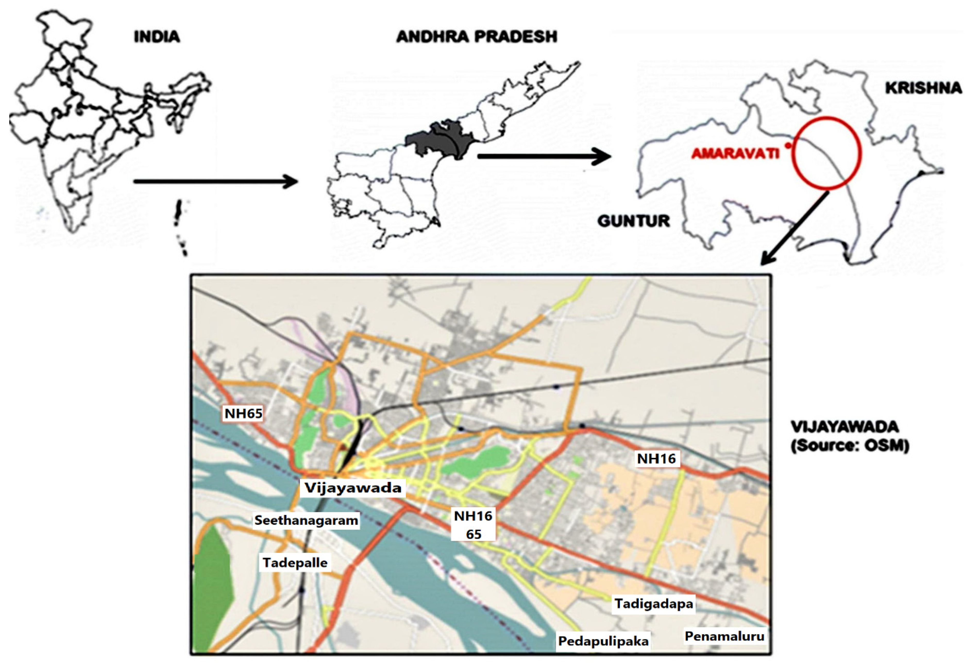
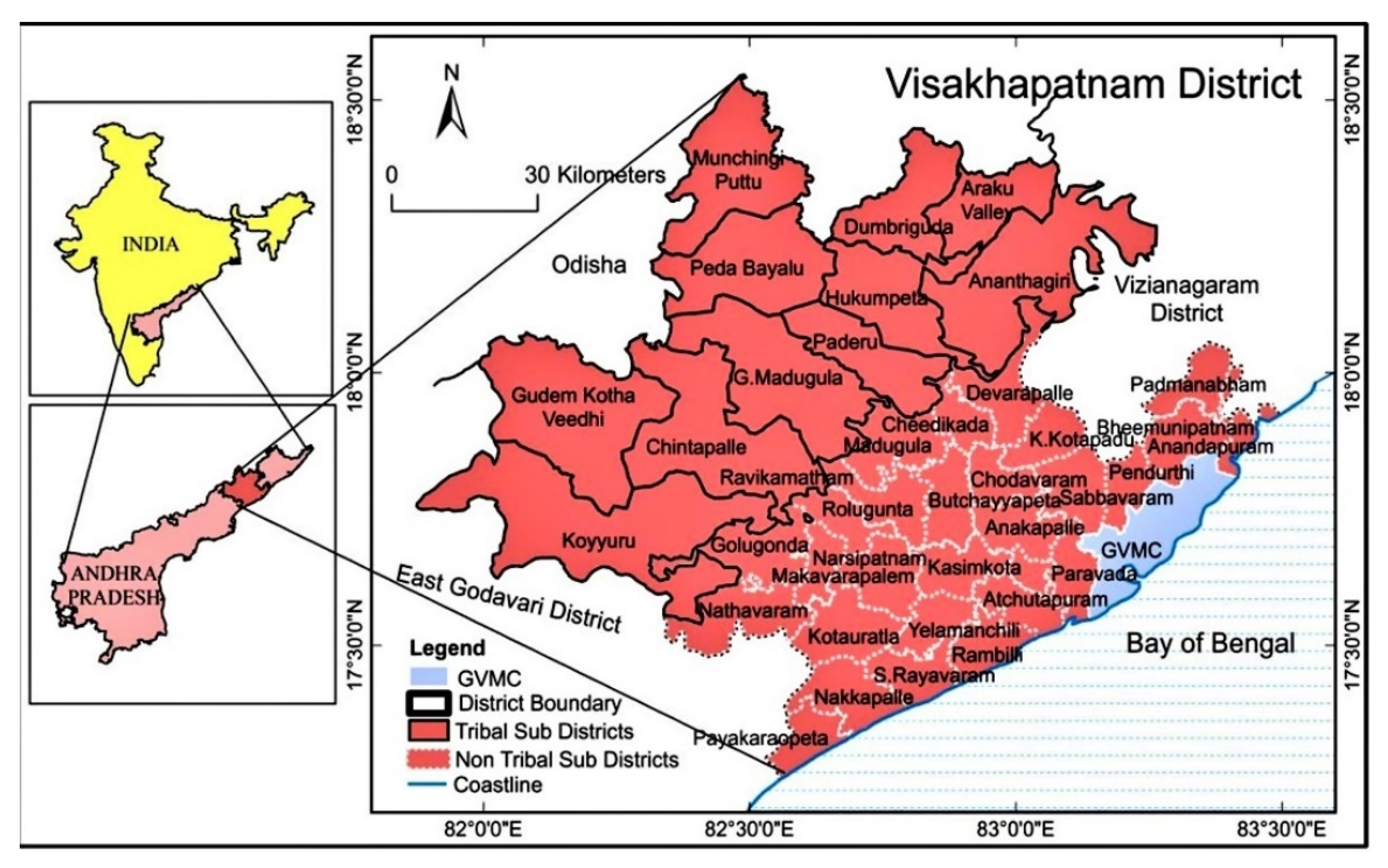
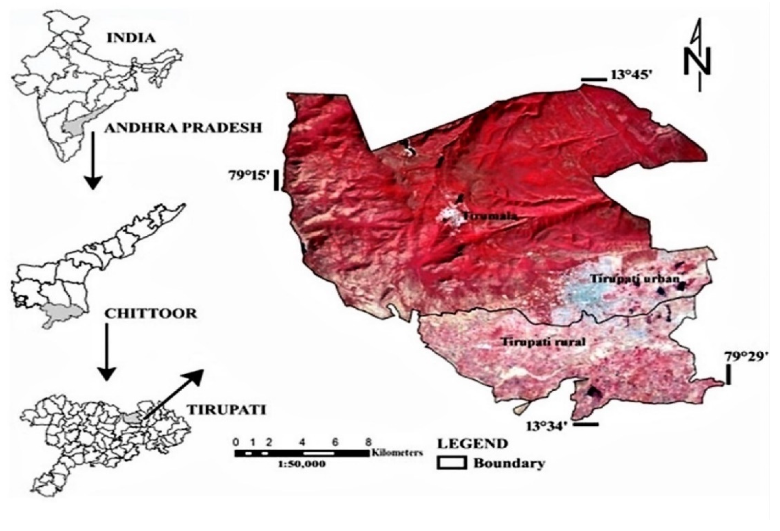
- To analyze LULC changes in Vijayawada, Visakhapatnam, and, Tirupati and assess spatio-temporal variations based on LULC changes.
- (ii)
- To analyze the transformation of surface temperature between vegetated and urbanized areas, correlating 20 years of considered data from LST, NDVI, and associated with the possible seasonal influences. The study shows the relationship between LST and NDVI during a rapid urbanization process, and how land use and land cover changes can affect this relationship.
2. Study Area
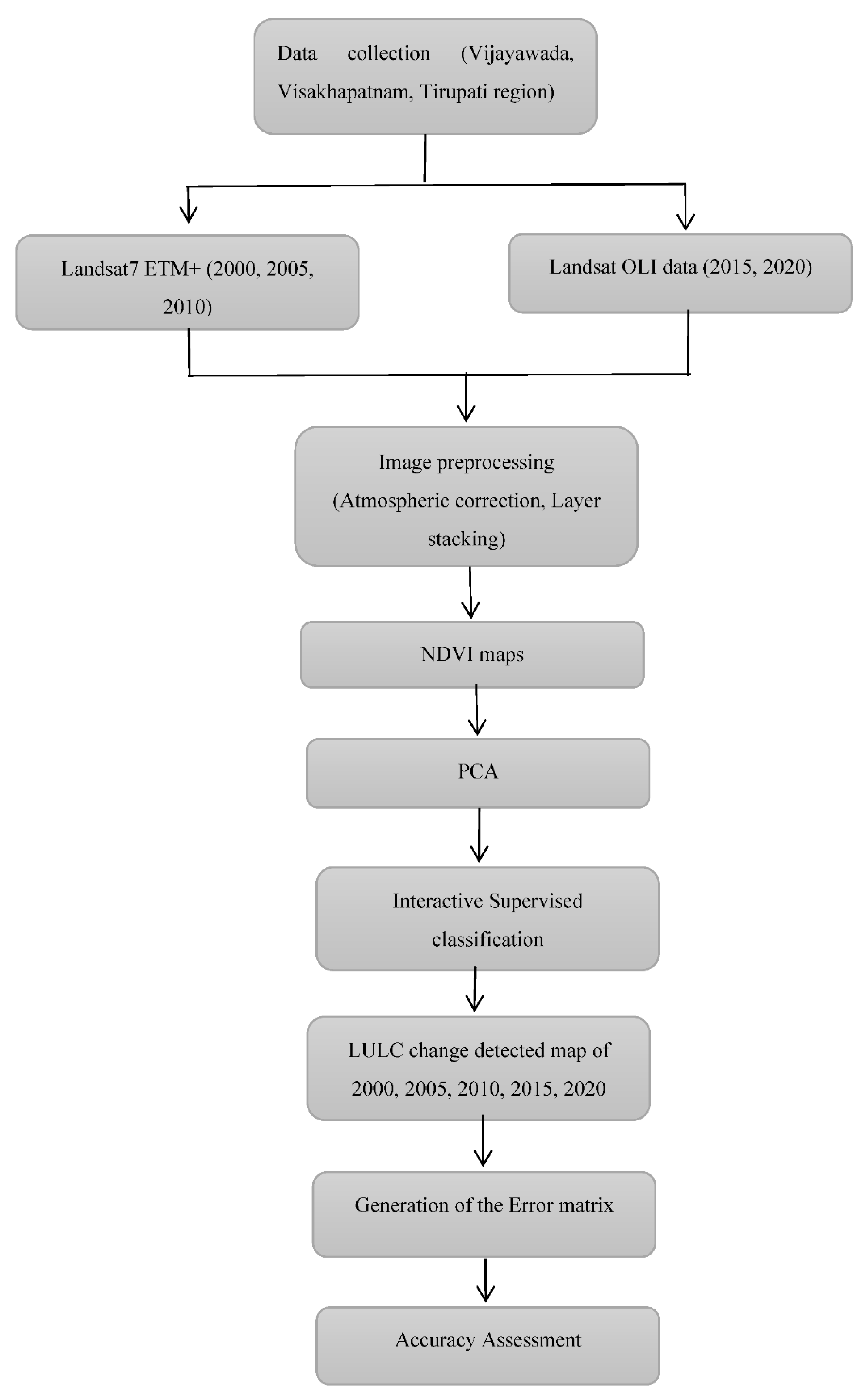
3. Methodology
3.1. Establishment of Temporal LULC Maps of the Survey Region
- 1.
- Calculate the mean of the image matrix, the mean vector being the vector average of the individual components of a vector (Equation (4)).
- 2.
- The covariance matrix is used to understand how the variables of the input data set vary from the mean for each other, something which is obtained by the equation (Equation (5)).
- 3.
- Eigenvectors and eigenvalues are the linear algebra concepts that are needed to compute from the covariance matrix to determine the principal components of the data. Eigenvalues (λ) can be obtained by the equation (Equation (6)).
- 4.
- Eigenvectors can be determined by the equation (Equation (7)).
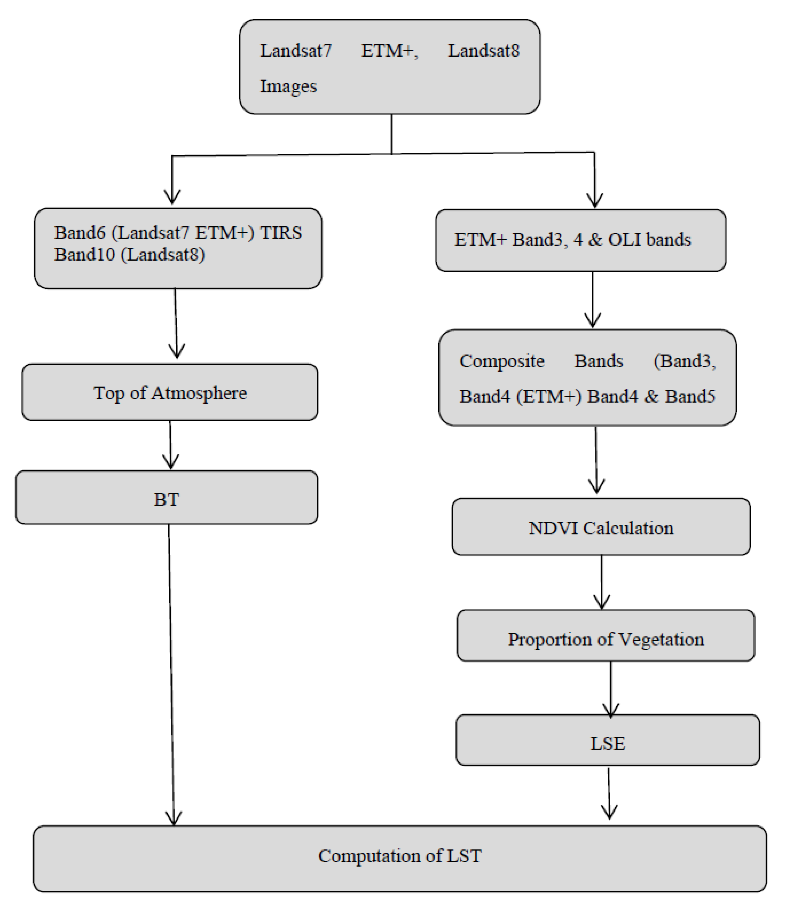
3.2. Computation of LST
4. Results
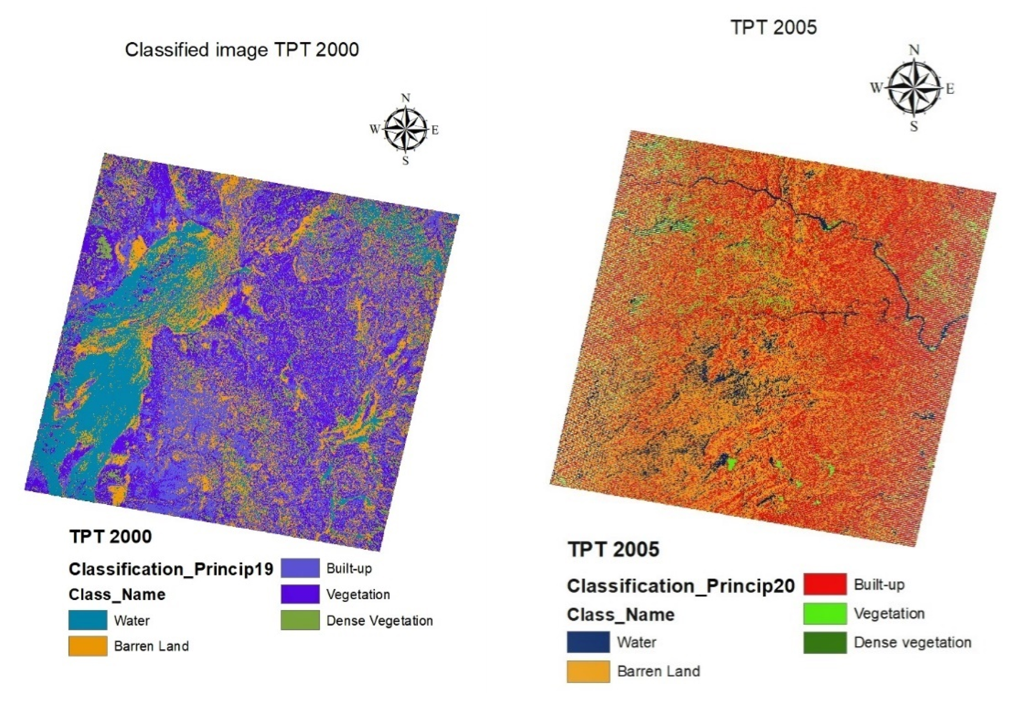
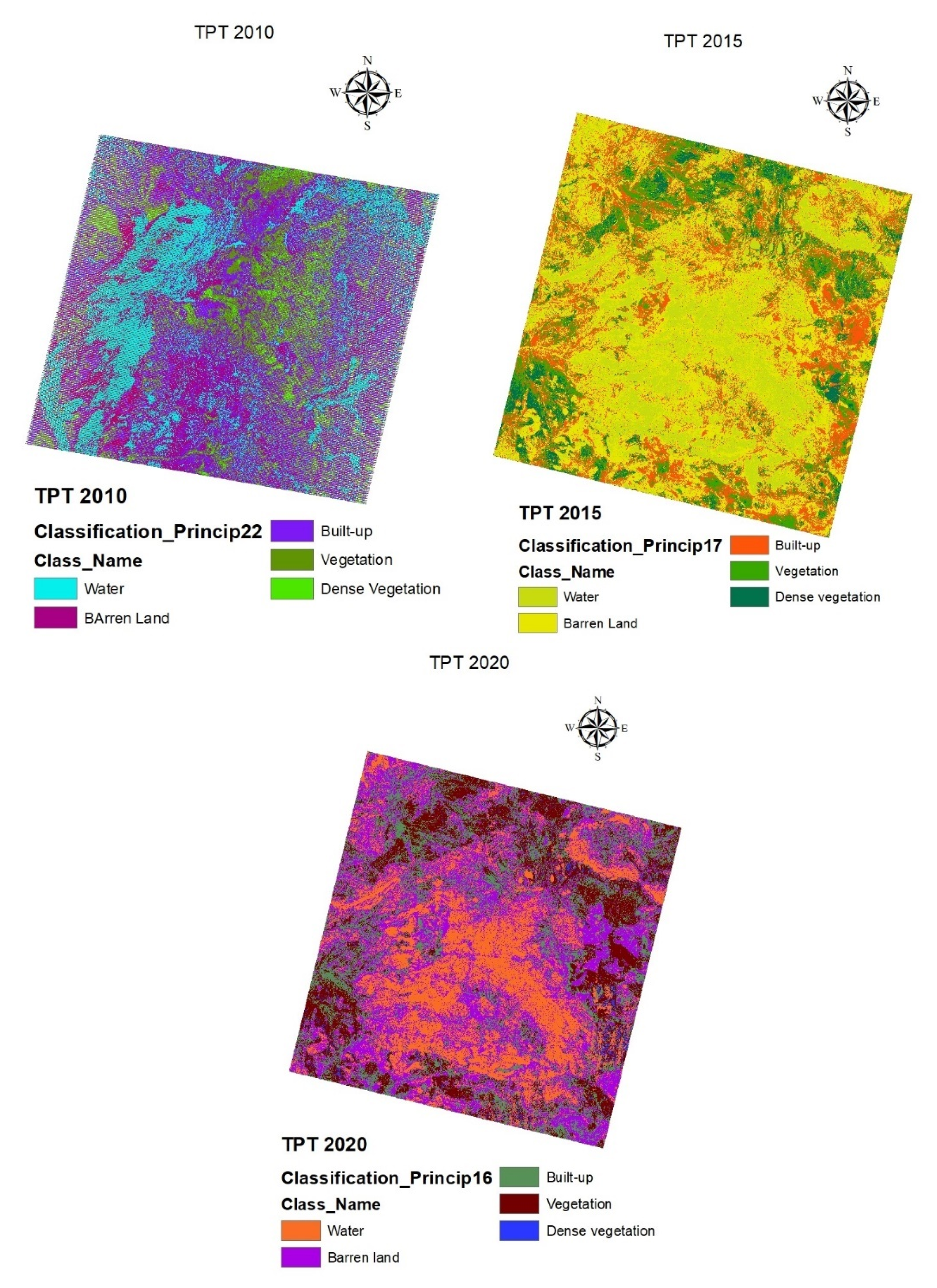
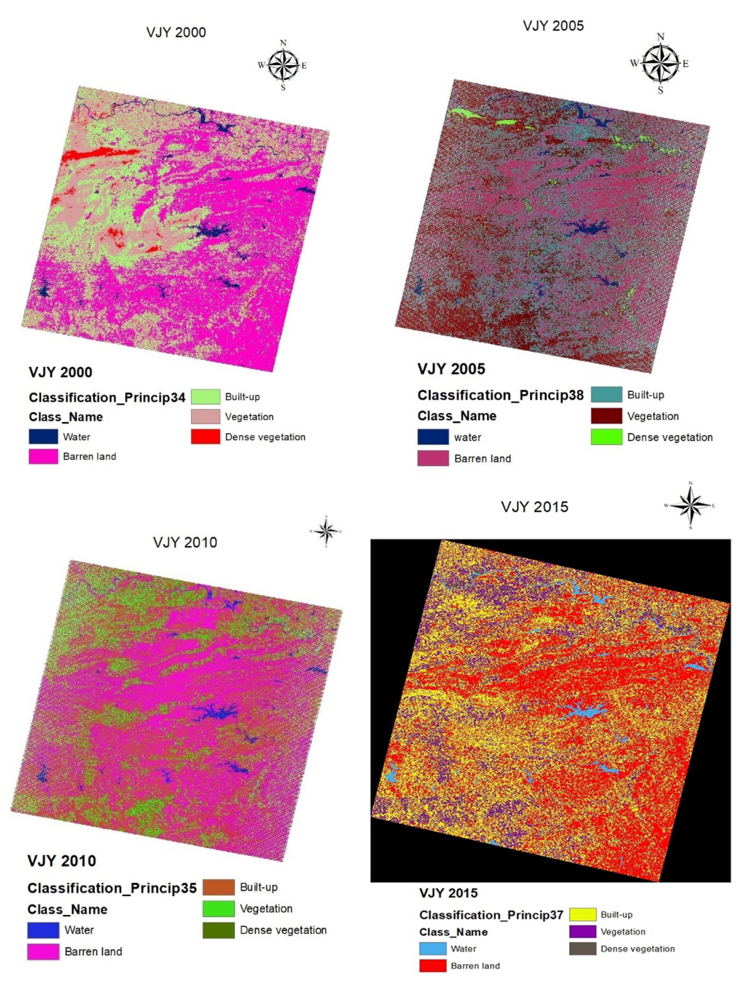
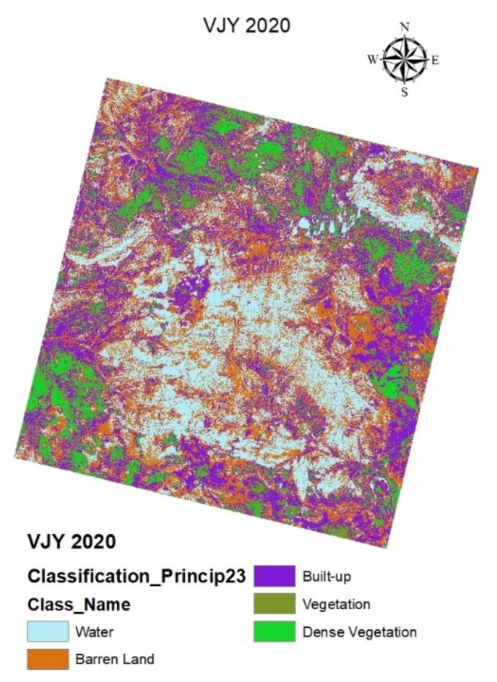
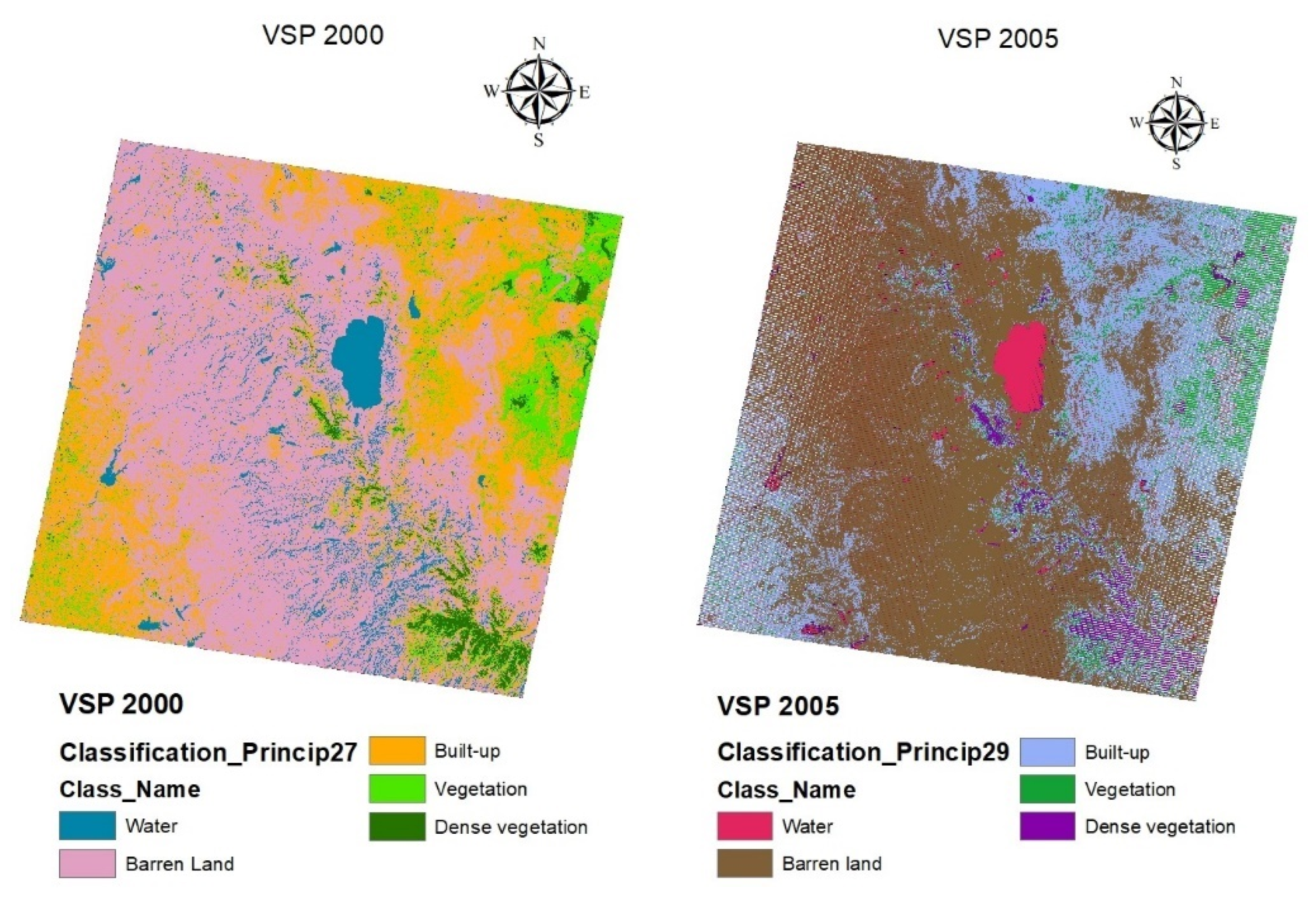
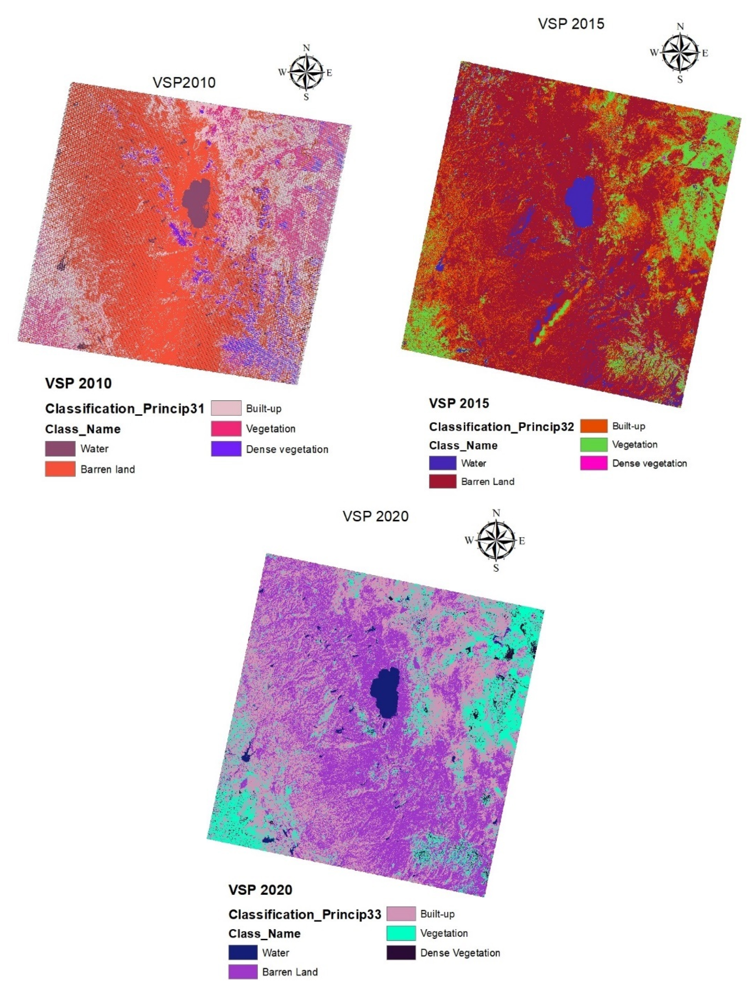
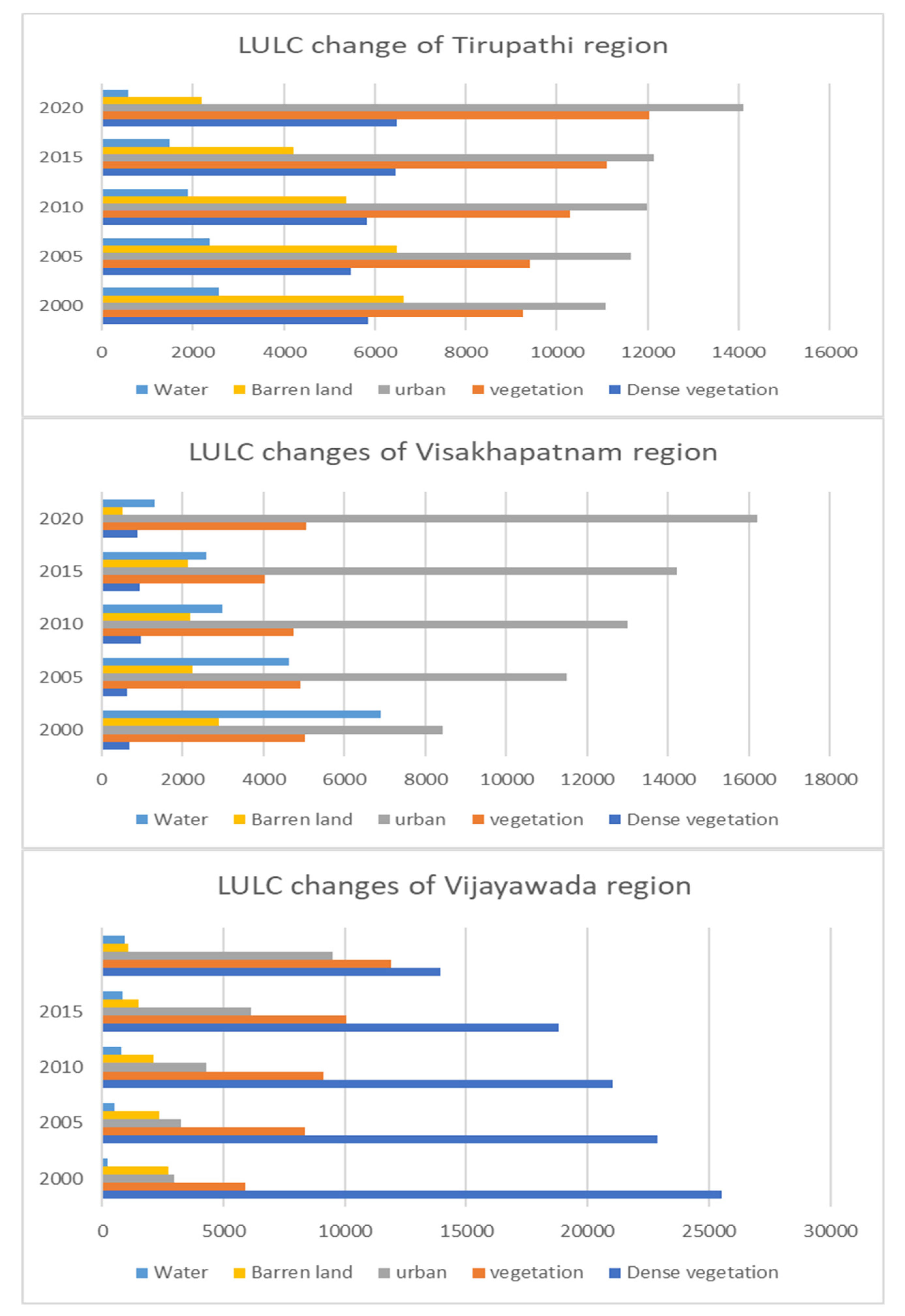
4.1. LULC Analysis
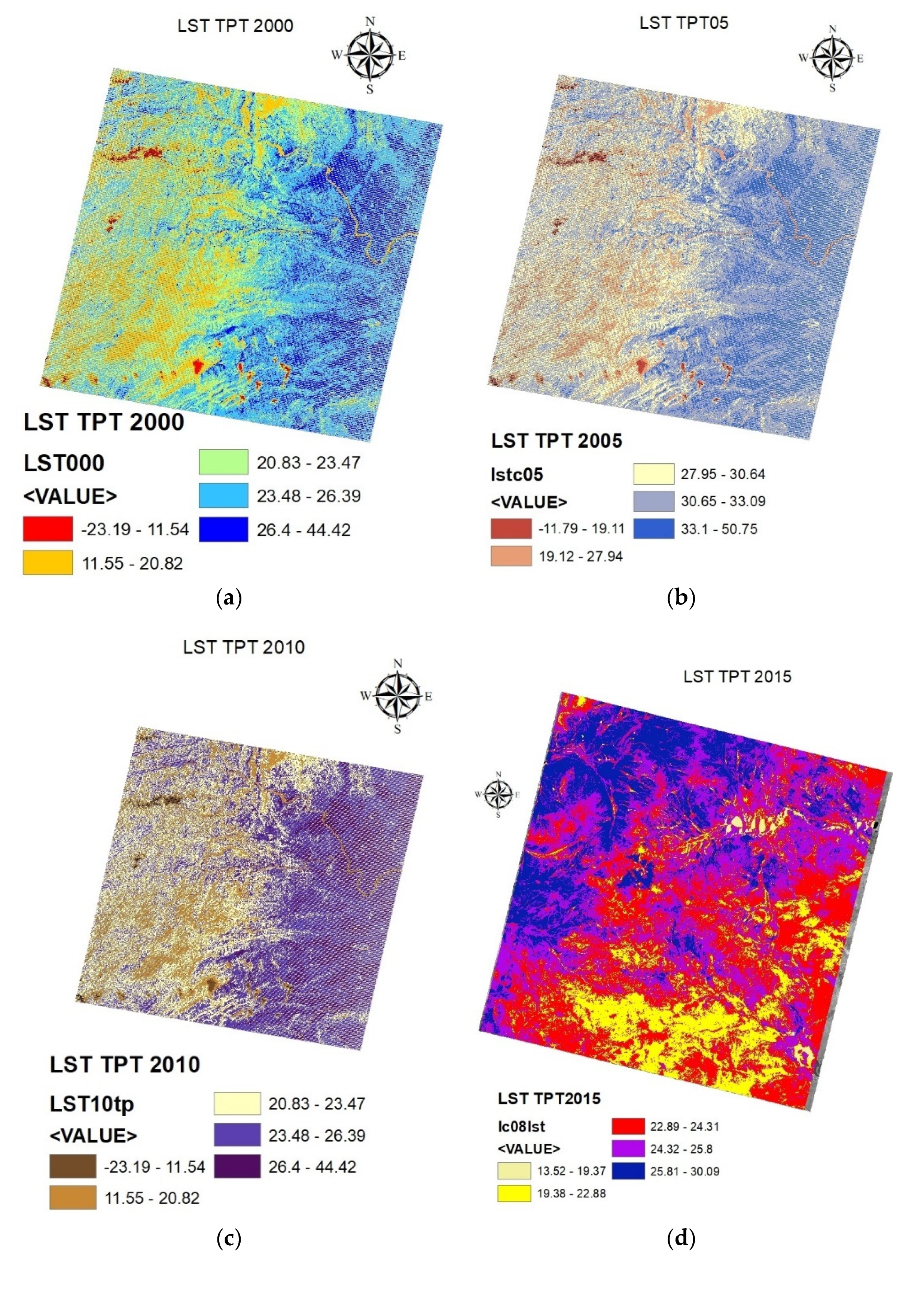
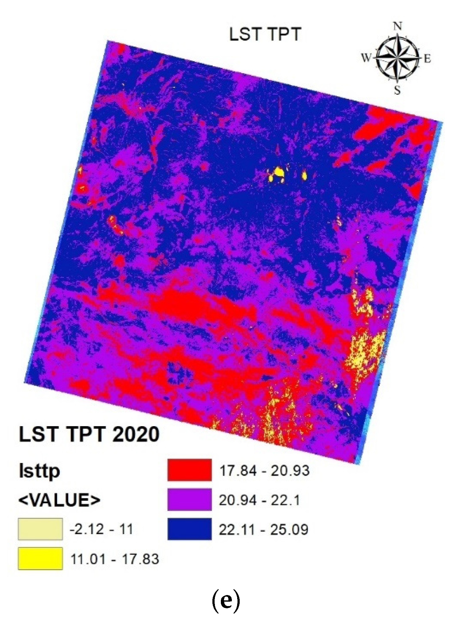
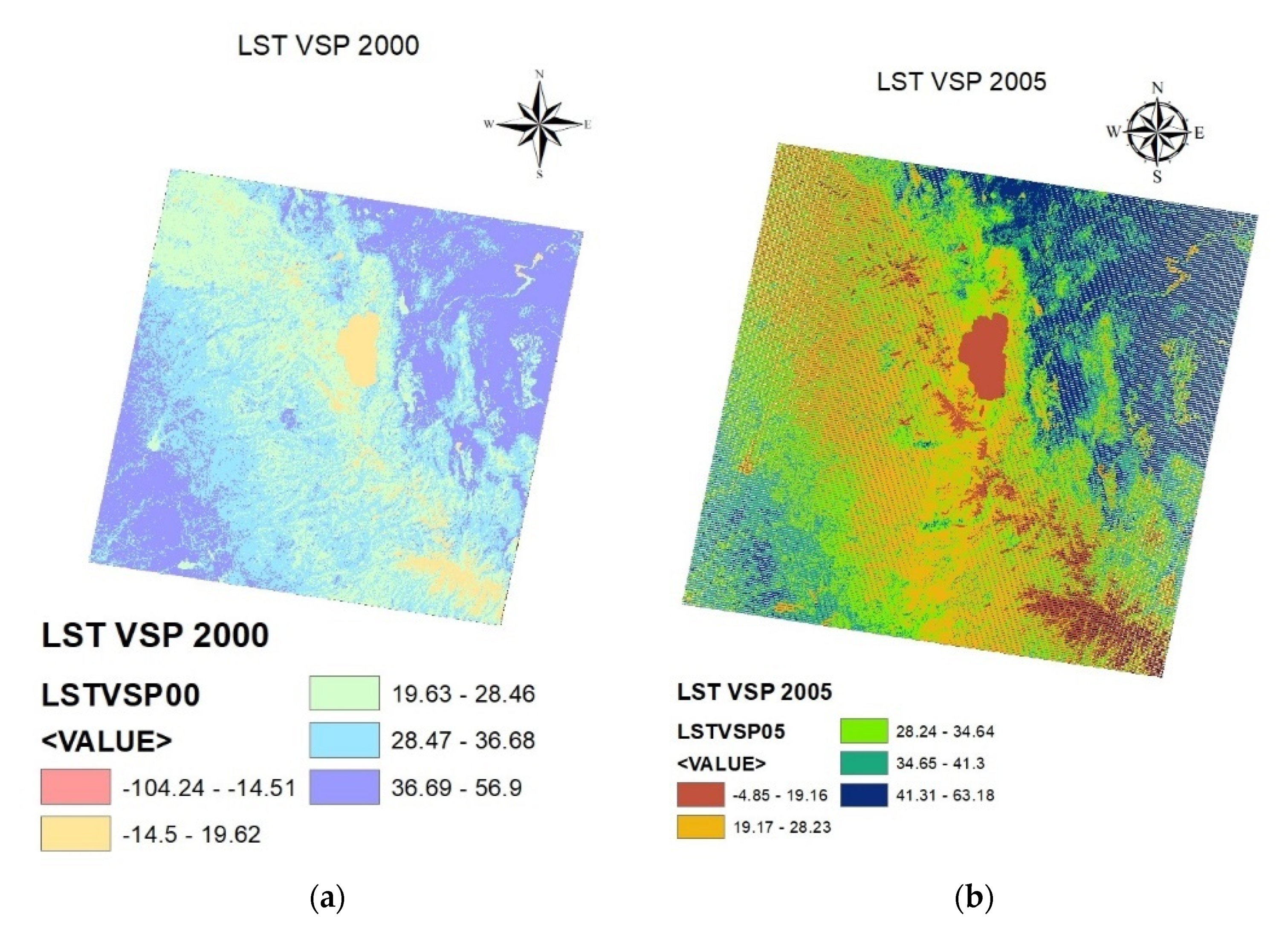
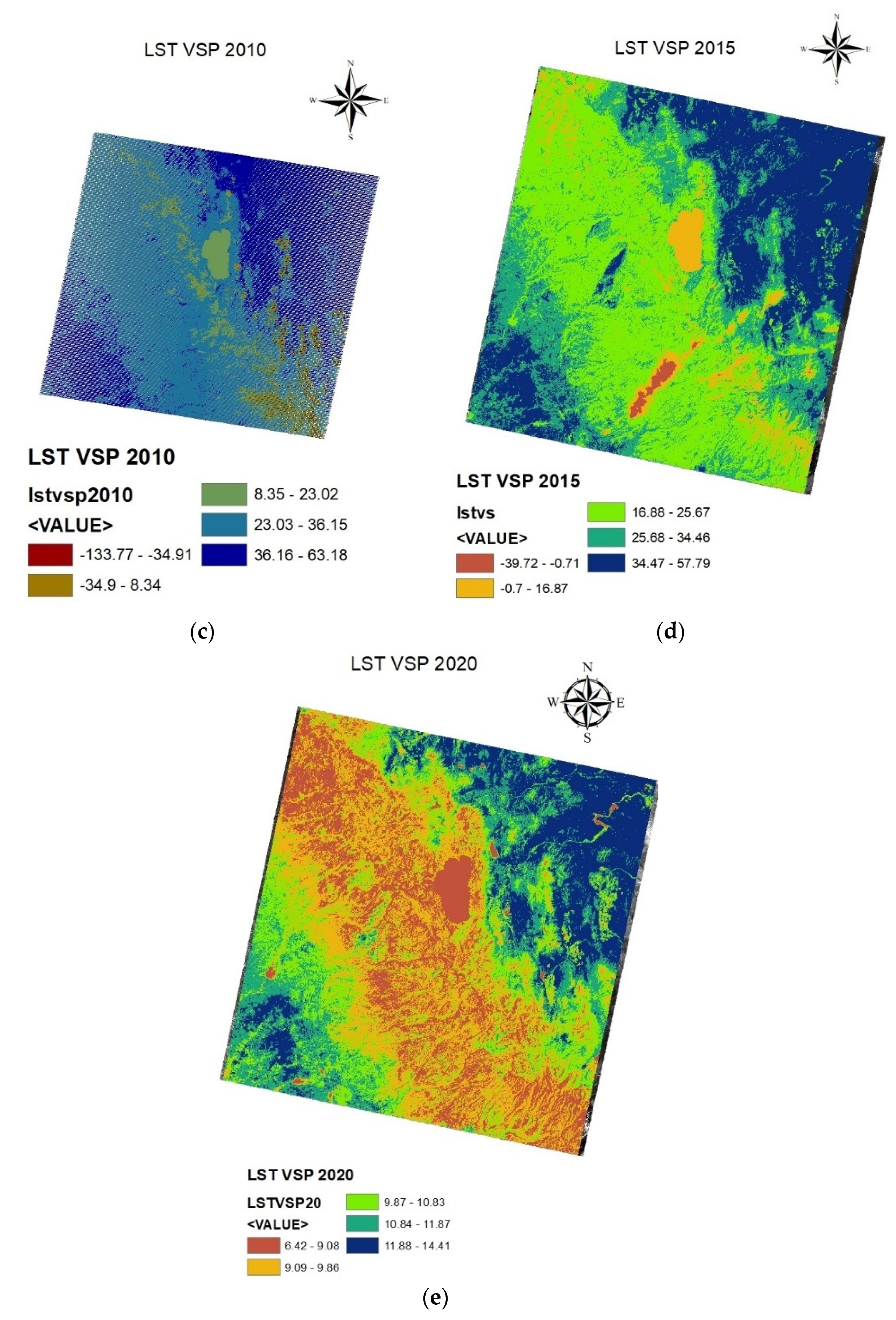
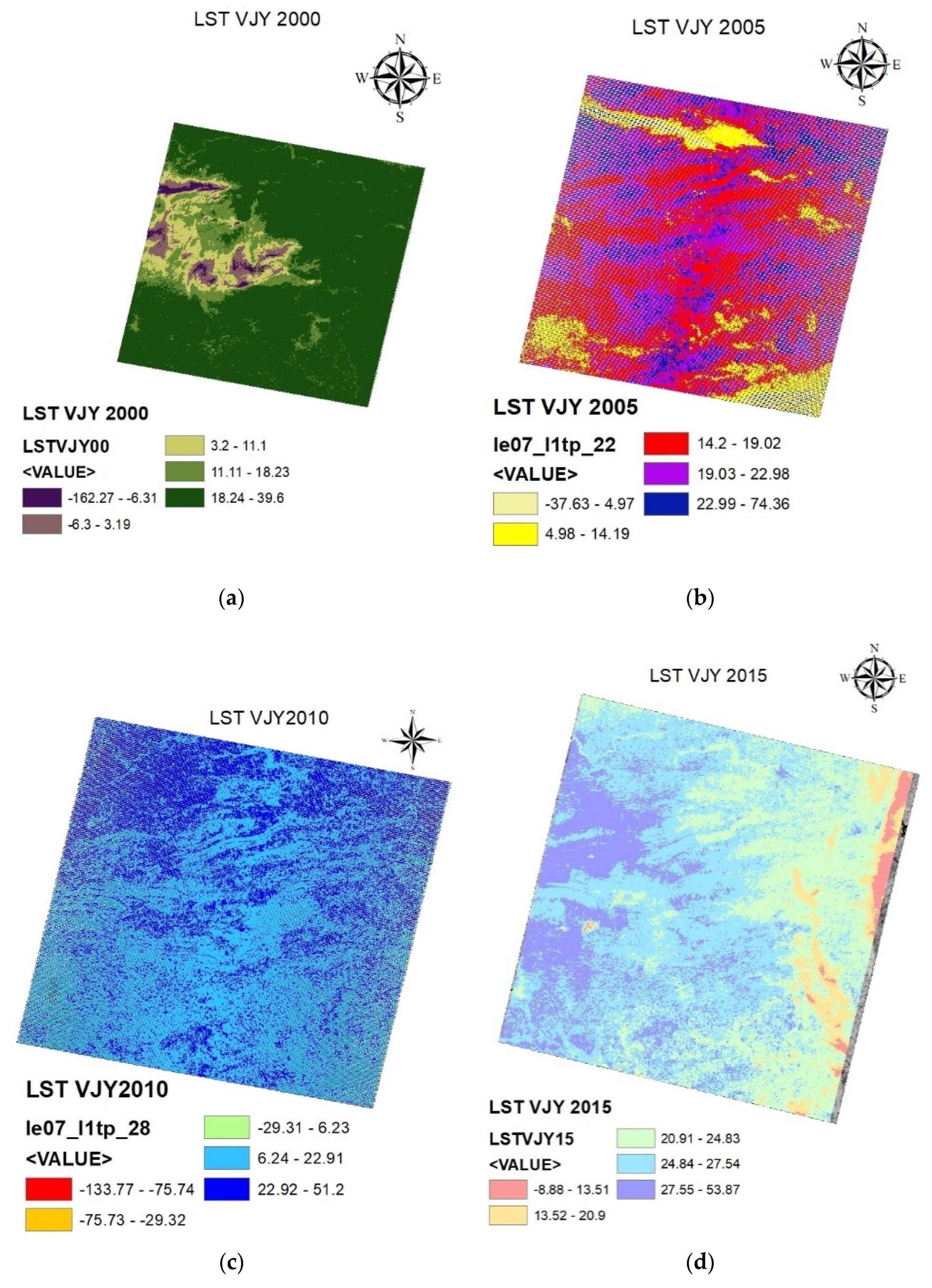
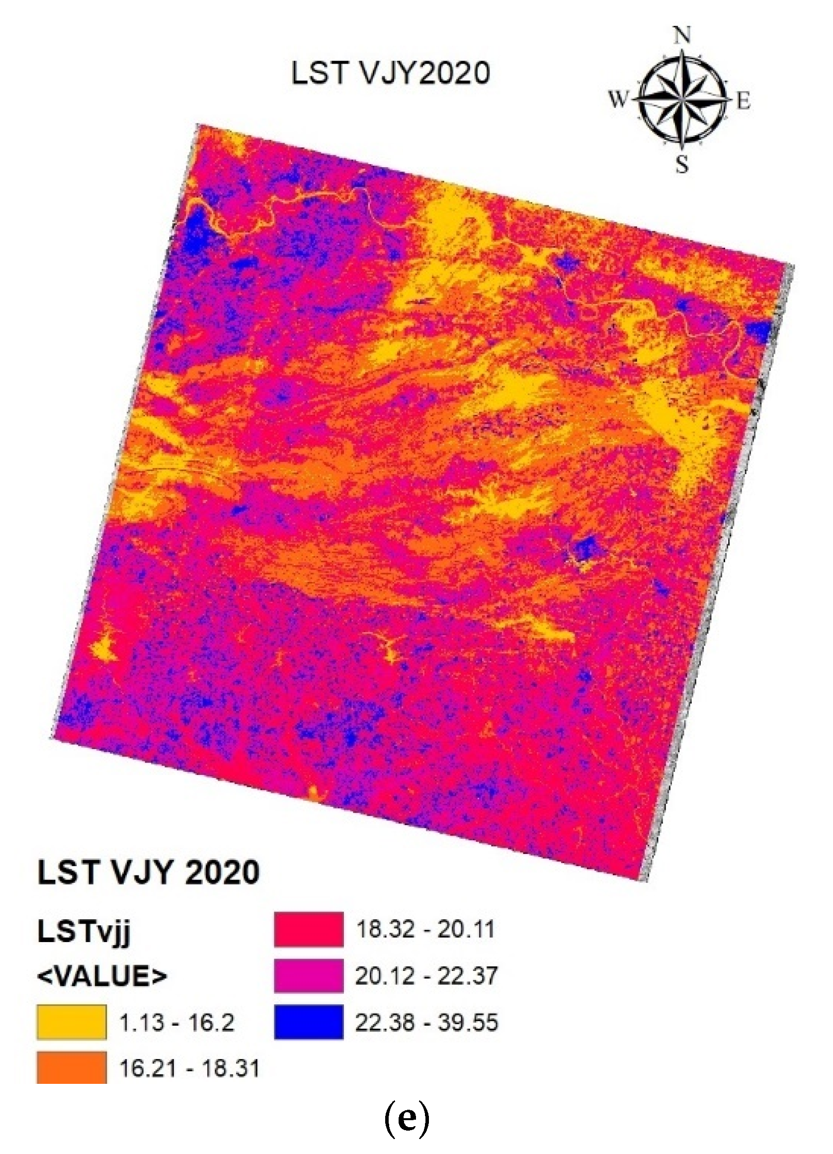
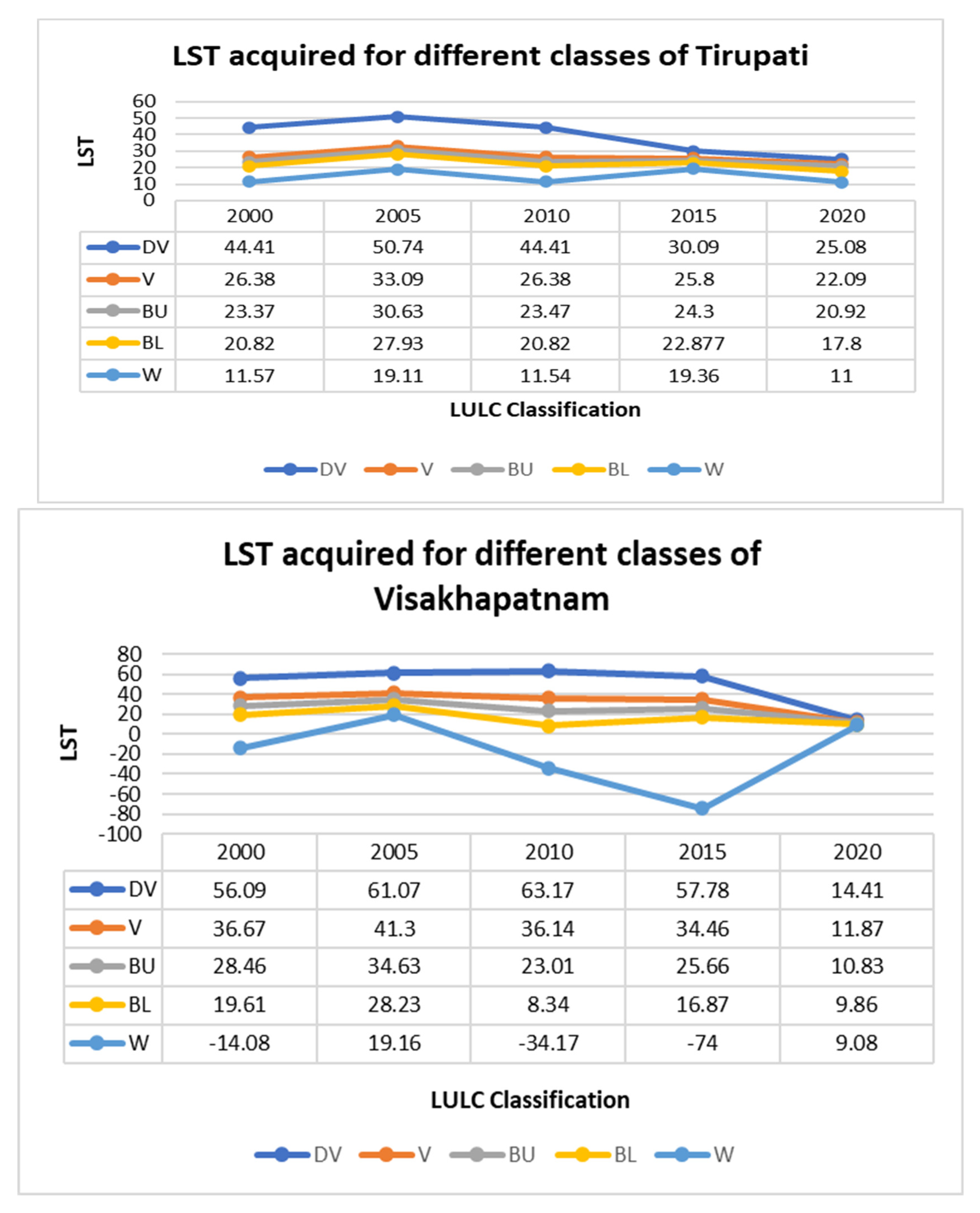
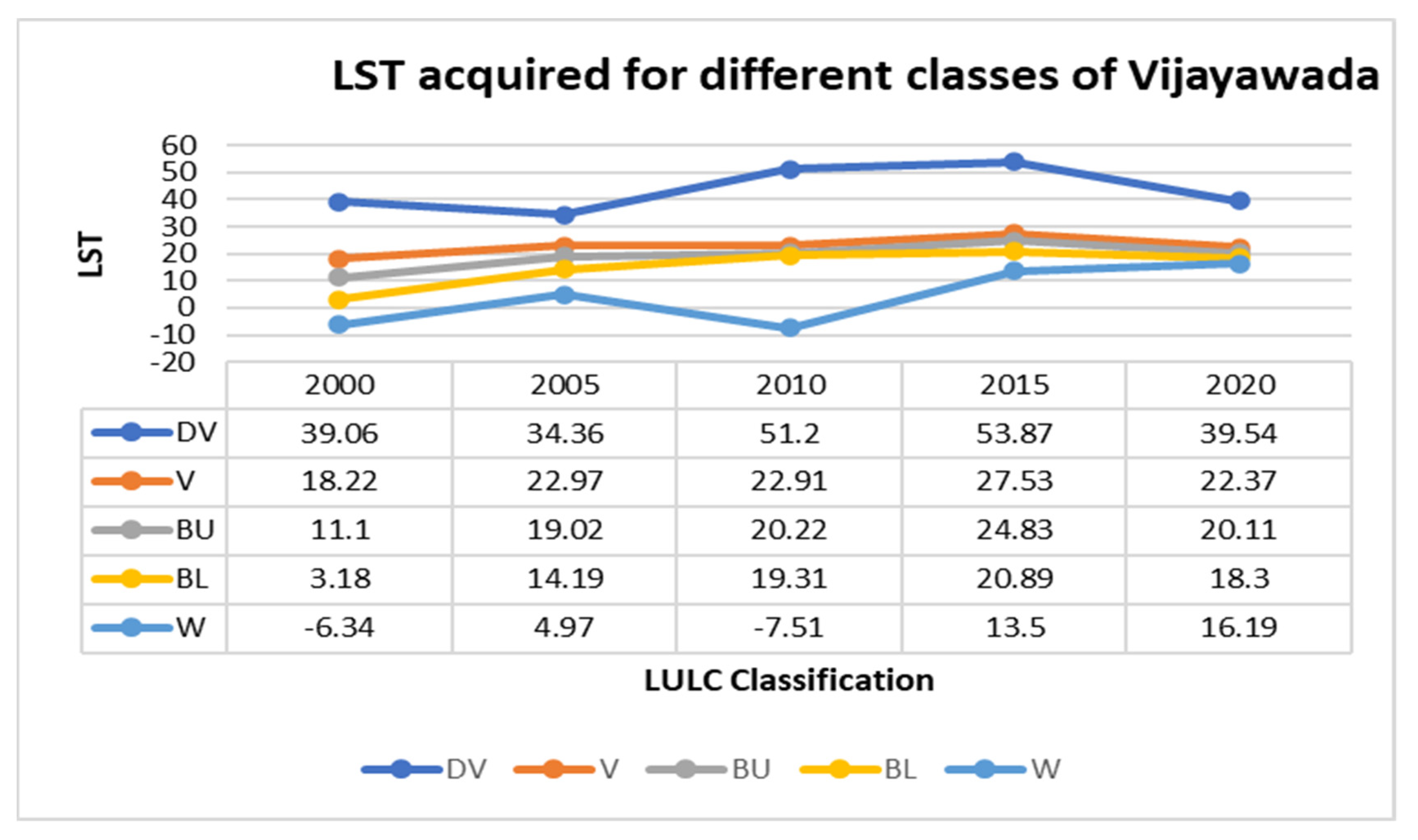
4.2. LST Analysis
5. Discussion
6. Conclusions
Author Contributions
Funding
Institutional Review Board Statement
Informed Consent Statement
Data Availability Statement
Conflicts of Interest
References
- Liping, C.; YuJun, S.; Saeed, S. Monitoring and predicting land use and land cover changes using remote sensing and GIS techniques—A case study of a hilly area, Jiangle, China. PLoS ONE 2018, 13, e0200493. [Google Scholar] [CrossRef] [PubMed]
- Rahaman, S.; Kumar, P.; Chen, R.; Meadows, M.E.; Singh, R.B. Remote Sensing Assessment of the Impact of Land Use and Land Cover Change on the Environment of Barddhaman District, West Bengal, India. Front. Environ. Sci. 2020, 8, 127. [Google Scholar] [CrossRef]
- Zhang, Y.; Zhao, H. Land–Use and Land-Cover Change Detection Using Dynamic Time Warping–Based Time Series Clustering Method. Can. J. Remote Sens. 2020, 46, 67–83. [Google Scholar] [CrossRef]
- Sexton, J.O.; Urban, D.L.; Donohue, M.J.; Song, C. Long-term land cover dynamics by multi-temporal classification across the Landsat-5 record. Remote Sens. Environ. 2013, 128, 246–258. [Google Scholar] [CrossRef]
- Vani, M.; Prasad, P.R.C. Assessment of spatio-temporal changes in land use and land cover, urban sprawl, and land surface temperature in and around Vijayawada city, India. Environ. Dev. Sustain. 2020, 22, 3079–3095. [Google Scholar] [CrossRef]
- Erle, E.; Robert, P. Land-use and land-cover change. In The Encyclopedia of Earth; Cleveland, C.J., Ed.; Environmental Information Coalition; National Council for Science and the Environment: Washington, DC, USA, 2010; pp. 142–153. [Google Scholar]
- Prakasam, C. Land use and land cover change detection through remote sensing approach: A case study of Kodaikanal taluk, Tamil Nadu. Int. J. Geomat. Geosci. 2010, 2, 150. [Google Scholar]
- Gupta, S.; Moupriya, R. Land Use/Land Cover classification of an urban area-A case study of Burdwan Municipality, India. Int. J. Geomat. Geosci. 2011, 4, 1014–1026. [Google Scholar]
- Quintas-Soriano, C.; Castro, A.J.; Castro, H.; García-Llorente, M. Impacts of land use change on ecosystem services and implications for human well-being in Spanish drylands. Land Use Policy 2016, 54, 534–548. [Google Scholar] [CrossRef]
- James, R.A. A Land Use and Land Cover Classification System for Use with Remote Sensor Data; US Government Printing Office: Washington, DC, USA, 1976; Volume 964, pp. 1–34.
- Brown, D.; Pijanowski, B.; Duh, J. Modeling the relationships between land use and land cover on private lands in the Upper Midwest, USA. J. Environ. Manag. 2000, 59, 247–263. [Google Scholar] [CrossRef]
- Sleeter, B.M.; Liu, J.; Daniel, C.; Rayfield, B.; Sherba, J.; Hawbaker, T.J.; Zhu, Z.; Selmants, P.C.; Loveland, T.R. Effects of contemporary land-use and land-cover change on the carbon balance of terrestrial ecosystems in the United States. Environ. Res. Lett. 2018, 13, 045006. [Google Scholar] [CrossRef]
- Miller, C.V.; Foster, G.D.; Majedi, B.F. Baseflow and stormflow metal fluxes from two small agricultural catchments in the Coastal Plain of the Chesapeake Bay Basin, United States. Appl. Geochem. 2003, 18, 483–501. [Google Scholar] [CrossRef]
- Fatemi, M.; Narangifard, M. Monitoring LULC changes and its impact on the LST and NDVI in District 1 of Shiraz City. Arab. J. Geosci. 2019, 12, 127. [Google Scholar] [CrossRef]
- Tan, K.C.; Lim, H.S.; MatJafri, M.Z.; Abdullah, K. Landsat data to evaluate urban expansion and determine land use/land cover changes in Penang Island, Malaysia. Environ. Earth Sci. 2010, 60, 1509–1521. [Google Scholar] [CrossRef]
- Al Kafy, A.-A.; Rahman, S.; Faisal, A.-A.; Hasan, M.M.; Islam, M. Modelling future land use land cover changes and their impacts on land surface temperatures in Rajshahi, Bangladesh. Remote Sens. Appl. Soc. Environ. 2020, 18, 100314. [Google Scholar]
- Pande, B.; Chaitanya, K.; Moharir, N.; Khadri, S.F.R. Assessment of land-use and land-cover changes in Pangari watershed area (MS), India, based on the remote sensing and GIS techniques. Appl. Water Sci. 2021, 11, 96. [Google Scholar] [CrossRef]
- Latha, M.H.; Varadarajan, S. Feature enhancement of multispectral images using vegetation, water, and soil indices image fusion. In Proceedings of the International Conference on ISMAC in Computational Vision and Bio-Engineering, Palladam, India, 16–17 May 2018; pp. 329–337. [Google Scholar]
- Baeza, S.; José, M.P. Land use/land cover change (2000–2014) in the Rio de la Plata grasslands: An analysis based on MODIS NDVI time series. Remote Sens. 2020, 12, 381. [Google Scholar] [CrossRef]
- Bonan, B.G. Forests and climate change: Forcings, feedbacks, and the climate benefits of forests. Science 2008, 320, 1444–1449. [Google Scholar] [CrossRef]
- Oliver, H.T.; Mike, D. Morecroft, Interactions between climate change and land-use change on biodiversity: Attribution problems, risks, and opportunities, Wiley Interdisciplinary Reviews. Clim. Chang. 2014, 5, 317–335. [Google Scholar]
- Goparaju, L. Geospatial Technology in Environmental Impact Assessments—Retrospective. Present Environ. Sustain. Dev. 2015, 9, 139–148. [Google Scholar] [CrossRef][Green Version]
- Ahmadi, M.; Mahdi, N. Land use change detection and its effects on the temperature range in the one Zone City of shiraz. J. Environ. Sci. 2015, 13, 111–120. [Google Scholar]
- Zhang, X.; Wang, D.; Hao, H.; Zhang, F.; Hu, Y. Effects of Land Use/Cover Changes and Urban Forest Configuration on Urban Heat Islands in a Loess Hilly Region: Case Study Based on Yan’an City, China. Int. J. Environ. Res. Public Health 2017, 14, 840. [Google Scholar] [CrossRef] [PubMed]
- Xing, H.; Zhu, L.; Chen, B.; Zhang, L.; Hou, D.; Fang, W. A novel change detection method using remotely sensed image time series value and shape based dynamic time warping. Geocarto Int. 2021, 1–18. [Google Scholar] [CrossRef]
- Alexander, C. Normalised difference spectral indices and urban land cover as indicators of land surface temperature (LST). Int. J. Appl. Earth Obs. Geoinf. 2020, 86, 102013. [Google Scholar] [CrossRef]
- Yangchen, U.; Ugyen, T.; Gudrun, W. Land use land cover changes in Bhutan: 2000–2013. In Proceedings of the International Conference on Climate Change, Environment and Development in Bhutan, Royal University of Bhutan (RUB), Thimphu, Bhutan, 2–3 April 2015; pp. 37–46. [Google Scholar]
- Dharani, M.; Sreenivasulu, G. Land use and land cover change detection using principal component analysis and morphological operations in remote sensing applications. Int. J. Comput. Appl. 2019, 43, 462–471. [Google Scholar] [CrossRef]
- Kogo, B.K.; Kumar, L.; Koech, R. Analysis of spatio-temporal dynamics of land use and cover changes in Western Kenya. Geocarto Int. 2021, 36, 376–391. [Google Scholar] [CrossRef]
- Kiranmai, S.V.; Ghai, D.; Kumar, S. A review on the classification of land use/land cover change assessment based on normalized difference vegetation index. J. Crit. Rev. 2020, 7, 2416–2431. [Google Scholar]
- Da Silva, V.S.; Salami, G.; Da Silva, M.I.O.; Silva, E.A.; Junior, J.J.M.; Alba, E. Methodological evaluation of vegetation indexes in land use and land cover (LULC) classification. Geol. Ecol. Landsc. 2020, 4, 159–169. [Google Scholar] [CrossRef]
- Shao, Z.; Sumari, N.S.; Portnov, A.; Ujoh, F.; Musakwa, W.; Mandela, P.J. Urban sprawl and its impact on sustainable urban development: A combination of remote sensing and social media data. Geo-Spat. Inf. Sci. 2021, 24, 241–255. [Google Scholar] [CrossRef]
- Dash, P.P.; Kakkar, R.; Shreenivas, V.; Prakash, P.J.; Mythri, D.J.; Kumar, K.H.V.; Singh, V.V.; Sahai, R.M.N. Quantification of Urban Expansion Using Geospatial Technology—A Case Study in Bangalore. Adv. Remote Sens. 2015, 4, 330–342. [Google Scholar] [CrossRef]
- Vivekananda, G.N.; Swathi, R.; Sujith, A.V.L.N. Multi-temporal image analysis for LULC classification and change detection. Eur. J. Remote Sens. 2021, 54, 189–199. [Google Scholar] [CrossRef]
- Vishwakarma, C.A.; Somnath, T.; Praveen, K.R.; Kamal, M.S.; Saumitra, M. Changing land trajectories: A case study from India using a remote sensing-based approach. Eur. J. Geogr. 2016, 7, 61–71. [Google Scholar]
- Sundarakumar, K.; Harika, M.; Begum, S.K.A.; Yamini, S.; Balakrishna, K. Land use and land cover change detection and urban sprawl analysis of Vijayawada city using multitemporal Landsat data. Int. J. Eng. Sci. Technol. 2012, 4, 170–178. [Google Scholar]
- Arveti, N.; Balaji, E.; Padmanava, D. Land use/land cover analysis based on various comprehensive geospatial data sets: A case study from Tirupati area, south India. Adv. Remote Sens. 2016, 5, 66473. [Google Scholar] [CrossRef]
- United Nations Population Fund (UNPF). Population, Resources and the Environment: The Critical Challenges; United Nations: New York, NY, USA, 1991. [Google Scholar]
- Sundara, K.; Bhaskar, U.; Padmakumari, K. Estimation of Land Surface Temperature to Study Urban Heat Island Effect Using Landsat Etm+ Image. Int. J. Eng. Sci. Technol. 2012, 4, 771–778. [Google Scholar]
- Yarrakula, K.; Kumar, K.S.; Krishna, K.L. Urban sprawl change detection analysis of Vijayawada city using multi-temporal remote sensing data. J. Chem. Pharm. Res. 2014, 11, 728–734. [Google Scholar]
- Rao, R.; Kumar, R. Land Cover classification Using Landsat-8 Optical Data and Supervised Classifiers. Int. J. Eng. Technol. 2018, 7, 101–104. [Google Scholar]
- Kiranmai, S.V.; Ghai, D.; Kumar, S. Land Use/Land Cover Change Analysis using NDVI, PCA. In Proceedings of the 2021 5th International Conference on Computing Methodologies and Communication IEEE, Erode, India, 8–10 April 2021; pp. 849–855. [Google Scholar]
- Available online: https://www.newindianexpress.com/states/andhra-pradesh/2020/jul/31/decks-cleared-for-three-capitals-in-andhra-pradesh-as-governor-gives-nod-to-bills-2177346.html (accessed on 31 July 2020).
- Andhra Pradesh Smart Cities to Be Ready by 2021. Available online: https://timesofindia.indiatimes.com/city/vijayawada/ap-smart-cities-to-be-ready-by-2021/articleshow/62286611.cms (accessed on 29 December 2017).
- Vishakhapatnam, India Page. Available online: http://www.fallingrain.com/world/IN/02/Vishakhapatnam.html (accessed on 12 December 2021).
- India Meteorological Department. Visakhapatnam Climatological Table Period: 1951–1980; Archived from the Original on 2 April 2015, Retrieved 25 March 2015; India Meteorological Department: New Delhi, India, 2015.
- Rajani, A.; Varadarajan, S. LU/LC change detection using NDVI & MLC through remote sensing and GIS for Kadapa region. In Cognitive Informatics and Soft Computing; Springer: Singapore, 2020; pp. 215–223. [Google Scholar]
- Lu, D.; Qihao, W. A survey of image classification methods and techniques for improving classification performance. Int. J. Remote Sens. 2007, 28, 823–870. [Google Scholar] [CrossRef]
- Dilawar, A.; Chen, B.; Trisurat, Y.; Tuankrua, V.; Arshad, A.; Hussain, Y.; Measho, S.; Guo, L.; Kayiranga, A.; Zhang, H.; et al. Spatiotemporal shifts in thermal climate in responses to urban cover changes: A-case analysis of major cities in Punjab, Pakistan. Geomatics. Nat. Hazards Risk 2021, 12, 763–793. [Google Scholar] [CrossRef]
- Guo, Y.-J.; Han, J.-J.; Zhao, X.; Dai, X.-Y.; Zhang, H. Understanding the Role of Optimized Land Use/Land Cover Components in Mitigating Summertime Intra-Surface Urban Heat Island Effect: A Study on Downtown Shanghai, China. Energies 2020, 13, 1678. [Google Scholar] [CrossRef]
- Qin, Z.; Karnieli, A. Progress in the remote sensing of land surface temperature and ground emissivity using NOAA-AVHRR data. Int. J. Remote Sens. 1999, 20, 2367–2393. [Google Scholar] [CrossRef]
- Lu, D.; Li, G.; Moran, E.; Hetrick, S. Spatiotemporal analysis of land-use and land-cover change in the Brazilian Amazon. Int. J. Remote Sens. 2013, 34, 5953–5978. [Google Scholar] [CrossRef] [PubMed]
- Rajani, A.; Varadarajan, S. Estimation and Validation of Land Surface Temperature by using Remote Sensing & GIS for Chittoor District, Andhra Pradesh. Turk. J. Comput. Math. Educ. 2021, 12, 607–617. [Google Scholar]
- Plourde, L.; Russell, G.C. Sampling method and sample placement. Photogramm. Eng. Remote Sens. 2003, 69, 289–297. [Google Scholar] [CrossRef]


| Area | Data Source | Sensor | PATH | ROW |
|---|---|---|---|---|
| Visakhapatnam | Landsat | ETM+, OLI/TIRS | 43 | 33 |
| Vijayawada | Landsat | ETM+, OLI/TIRS | 25 | 36 |
| Tirupati | Landsat | ETM+, OLI/TIRS | 96 | 78 |
| Constants | ETM+ | OLI |
|---|---|---|
| K1 | 666.09 | 774.8853 |
| K2 | 1282.71 | 1321.0789 |
| Lmax | 12.65 | 22.00180 |
| Lmin | 3.200 | 0.10033 |
| Qcal max | 255 | 65,535 |
| Qcal min | 1 | 1 |
| LULC Category | Area (Hectares) | Change in Area (Hectares) | Change in Area (%) | |||||||||
|---|---|---|---|---|---|---|---|---|---|---|---|---|
| Year (2000) | Area (%) | Year (2005) | Area (%) | Year (2010) | Area (%) | Year (2015) | Area (%) | Year (2020) | Area (%) | |||
| Dense vegetation | 5857.62 | 16.54 | 5482.53 | 15.49 | 5828.29 | 16.47 | 6467.46 | 18.27 | 6490.25 | 18.34 | 632.63 | 1.80 |
| Vegetation | 9268.07 | 26.18 | 9419.84 | 26.61 | 10,300.05 | 29.10 | 11,090.49 | 31.33 | 12,023.85 | 33.97 | 2755.78 | 7.79 |
| Urban | 11,074.08 | 31.28 | 11,637.09 | 32.88 | 11,981.78 | 33.85 | 12,129.59 | 34.27 | 14,094.56 | 39.82 | 3020.48 | 8.54 |
| Barren Land | 6629.97 | 18.73 | 6491.48 | 18.34 | 5380.86 | 15.20 | 4206.45 | 11.88 | 2205.70 | 6.23 | −4424.27 | −12.50 |
| Water | 2564.62 | 7.2 | 2363.42 | 6.68 | 1903.38 | 5.38 | 1500.38 | 4.24 | 579.99 | 1.64 | −1984.63 | −5.56 |
| Total | 35,394.38 | 35,394.38 | 35,394.38 | 35,394.38 | 35,394.38 | |||||||
| LULC Category | Area (Hectares) | Change in Area (Hectares) | Change in Area (%) | |||||||||
|---|---|---|---|---|---|---|---|---|---|---|---|---|
| Year (2000) | Area (%) | Year (2005) | Area (%) | Year (2010) | Area (%) | Year (2015) | Area (%) | Year (2020) | Area (%) | |||
| Dense vegetation | 688.04 | 2.88 | 630.83 | 2.64 | 973.39 | 4.07 | 925.48 | 3.87 | 880.28 | 3.68 | 192.24 | 0.80 |
| Vegetation | 5018.57 | 20.99 | 4910.27 | 20.53 | 4750.29 | 19.86 | 4040.93 | 16.90 | 5037.82 | 21.07 | 19.25 | 0.08 |
| Urban | 8425.71 | 35.23 | 11,501.08 | 48.09 | 12,997.44 | 54.35 | 14,221.88 | 59.47 | 16,200.84 | 67.75 | 7775.67 | 32.51 |
| Barren Land | 2888.00 | 12.08 | 2240.47 | 9.37 | 2198.72 | 9.19 | 2140.62 | 8.95 | 501.67 | 2.10 | −2386.33 | −9.98 |
| Water | 6893.29 | 28.83 | 4630.96 | 19.37 | 2993.76 | 12.52 | 2584.70 | 10.81 | 1292.99 | 5.41 | −5600.27 | −23.42 |
| Total | 23,913.62 | 23,913.62 | 23,913.62 | 23,913.62 | 23,913.62 | |||||||
| LULC Category | Area (Hectares) | Change in Area (Hectares) | change in Area (%) | |||||||||
|---|---|---|---|---|---|---|---|---|---|---|---|---|
| Year (2000) | Area (%) | Year (2005) | Area (%) | Year (2010) | Area (%) | Year (2015) | Area (%) | Year (2020) | Area (%) | |||
| Dense vegetation | 25,517.5 | 68.34 | 22,889 | 61.30 | 21,013.5 | 56.28 | 18,801.5 | 50.35 | 13,950.27 | 37.36 | −11,567.23 | −30.98 |
| Vegetation | 5908.07 | 15.82 | 8350.53 | 22.36 | 9136.9 | 24.47 | 10,045.1 | 26.90 | 11,898.7 | 31.87 | 5990.63 | 16.04 |
| Urban | 2950.24 | 7.90 | 3259.73 | 8.73 | 4288.4 | 11.48 | 6122.5 | 16.40 | 9503.3 | 25.45 | 6553.06 | 17.55 |
| Barren Land | 2754.47 | 7.38 | 2332.37 | 6.25 | 2123.17 | 5.69 | 1515.27 | 4.06 | 1075.1 | 2.88 | −1679.37 | −4.50 |
| Water | 209.09 | 0.56 | 507.74 | 1.36 | 777.4 | 2.08 | 855 | 2.29 | 912 | 2.44 | 702.91 | 1.88 |
| Total | 37,339.37 | 37,339.37 | 37,339.37 | 37,339.37 | 37,339.37 | |||||||
| Class ID | Reference Data | |||||||||||
|---|---|---|---|---|---|---|---|---|---|---|---|---|
| 1 | 2 | 3 | 4 | 5 | Ground Truth Points | User’s Accuracy (%) | Error of Commission | Specificity | F-Score (%) | False-Positive Rate | ||
| Classified Data | 1 | 98 | 3 | 2 | 0 | 0 | 103 | 95.1 | 4.8 | 0.98 | 95.5 | 0.02 |
| 2 | 4 | 96 | 2 | 0 | 0 | 102 | 94.1 | 5.8 | 0.98 | 94.1 | 0.02 | |
| 3 | 0 | 3 | 90 | 0 | 0 | 93 | 96.7 | 3.2 | 0.98 | 94.6 | 0.02 | |
| 4 | 0 | 0 | 3 | 91 | 0 | 94 | 96.8 | 3.1 | 1 | 98.3 | 0 | |
| 5 | 0 | 0 | 0 | 0 | 89 | 89 | 100 | 0 | 1 | 100 | 0 | |
| Ground truth points | 102 | 102 | 97 | 91 | 89 | 481 | ||||||
| Producer’s Accuracy (%) | 96 | 94.1 | 92.7 | 100 | 100 | |||||||
| Error of Omission | 3.9 | 5.8 | 7.2 | 0 | 0 | |||||||
| Region of Interest | 2000 | 2005 | 2010 | 2015 | 2020 | |||||
|---|---|---|---|---|---|---|---|---|---|---|
| Overall Accuracy (%) | Kappa Coefficient | Overall Accuracy (%) | Kappa Coefficient | Overall Accuracy (%) | Kappa Coefficient | Overall Accuracy (%) | Kappa Coefficient | Overall Accuracy (%) | Kappa Coefficient | |
| Vijayawada (VJY) | 88 | 0.86 | 91.5 | 0.89 | 93 | 0.91 | 94.5 | 0.93 | 96.4 | 0.95 |
| Visakhapatnam (VSP) | 89.3 | 0.87 | 92.5 | 0.9 | 93 | 0.91 | 94.5 | 0.92 | 97 | 0.96 |
| Tirupati (TPT) | 90.4 | 0.89 | 91 | 0.9 | 92.5 | 0.91 | 94.5 | 0.92 | 96.8 | 0.96 |
| Type of Land Cover | 2000 | 2005 | 2010 | 2015 | 2020 | ||||||||||
|---|---|---|---|---|---|---|---|---|---|---|---|---|---|---|---|
| VJY | VSP | TPT | VJY | VSP | TPT | VJY | VSP | TPT | VJY | VSP | TPT | VJY | VSP | TPT | |
| 1 | 87.5 | 86.8 | 89.1 | 91.8 | 91.2 | 90 | 92.5 | 92.5 | 91.2 | 93.8 | 93.8 | 93.8 | 95.1 | 97.6 | 99 |
| 2 | 89.4 | 88.6 | 89.4 | 92.7 | 89.6 | 93.8 | 91 | 91 | 89.6 | 94.4 | 93 | 93 | 94.1 | 96.4 | 95.2 |
| 3 | 85.3 | 88.7 | 88.7 | 88.8 | 92 | 90.9 | 92 | 92 | 92 | 91.6 | 94.8 | 94.8 | 96.7 | 98.8 | 97 |
| 4 | 87.5 | 91.6 | 91.6 | 92.7 | 95.8 | 90.7 | 95.8 | 95.8 | 95.8 | 96.2 | 94.8 | 94.8 | 96.8 | 96.4 | 97 |
| 5 | 91.8 | 91 | 93.4 | 91.3 | 93.9 | 91.3 | 94 | 94 | 93.9 | 97 | 95.9 | 95.9 | 100 | 97.6 | 97.8 |
| Type of Land Cover | 2000 | 2005 | 2010 | 2015 | 2020 | ||||||||||
|---|---|---|---|---|---|---|---|---|---|---|---|---|---|---|---|
| VJY | VSP | TPT | VJY | VSP | TPT | VJY | VSP | TPT | VJY | VSP | TPT | VJY | VSP | TPT | |
| 1 | 92.5 | 92.7 | 92.7 | 96.7 | 93.1 | 96.7 | 93.1 | 93.1 | 93.1 | 95.8 | 97.8 | 97.8 | 96 | 97.6 | 98 |
| 2 | 80.8 | 83.3 | 83.3 | 85.7 | 88.4 | 87.6 | 88.5 | 88.5 | 88.4 | 89.4 | 93.9 | 93.9 | 94.1 | 97.6 | 97 |
| 3 | 82.6 | 85.9 | 85.9 | 88 | 90.1 | 85.7 | 92.6 | 92.6 | 90.1 | 94.9 | 88.5 | 88.5 | 92.7 | 97.6 | 95 |
| 4 | 92.9 | 93.2 | 93.2 | 90.8 | 91.5 | 90.7 | 91.5 | 91.5 | 91.5 | 93.5 | 94.8 | 94.8 | 100 | 96.4 | 98 |
| 5 | 94.1 | 98.2 | 98.2 | 97.7 | 100 | 97.7 | 100 | 100 | 100 | 100 | 98 | 98 | 100 | 97.6 | 96 |
| Type of Land Cover | 2000 | 2005 | 2010 | 2015 | 2020 | ||||||||||
|---|---|---|---|---|---|---|---|---|---|---|---|---|---|---|---|
| VJY | VSP | TPT | VJY | VSP | TPT | VJY | VSP | TPT | VJY | VSP | TPT | VJY | VSP | TPT | |
| 1 | 12.5 | 13.1 | 10.85 | 8.1 | 8.7 | 10 | 7.4 | 7.4 | 8.7 | 6.1 | 6.1 | 6.1 | 4.8 | 2.3 | 1 |
| 2 | 10.5 | 11.3 | 10.56 | 7.2 | 10.3 | 6.1 | 8.9 | 8.9 | 10.3 | 5.5 | 7 | 7 | 5.8 | 3.5 | 6.5 |
| 3 | 14.6 | 11.2 | 11.29 | 11.1 | 8 | 9 | 8 | 8 | 8 | 8.3 | 5.1 | 5.1 | 3.2 | 1.1 | 3 |
| 4 | 12.5 | 8.3 | 8.33 | 7.2 | 4.1 | 9.2 | 4.1 | 4.1 | 4.1 | 3.7 | 5.1 | 5.1 | 3.1 | 3.5 | 3 |
| 5 | 8.13 | 8.9 | 6.5 | 8.6 | 6 | 8.6 | 6 | 6 | 6 | 3 | 4 | 4 | 0 | 2.3 | 2.1 |
| Type of Land Cover | 2000 | 2005 | 2010 | 2015 | 2020 | ||||||||||
|---|---|---|---|---|---|---|---|---|---|---|---|---|---|---|---|
| VJY | VSP | TPT | VJY | VSP | TPT | VJY | VSP | TPT | VJY | VSP | TPT | VJY | VSP | TPT | |
| 1 | 7.4 | 7.2 | 7.2 | 3.2 | 6.8 | 3.2 | 6.8 | 6.8 | 6.8 | 4.1 | 2.1 | 2.1 | 3.9 | 2.3 | 2 |
| 2 | 19.1 | 16.6 | 16.6 | 14.2 | 11.5 | 12.3 | 11.4 | 11.4 | 11.5 | 4.6 | 6.1 | 6.1 | 5.8 | 2.3 | 3 |
| 3 | 17.3 | 14 | 14 | 12 | 9.8 | 14.2 | 7.3 | 7.3 | 9.8 | 5.1 | 11.4 | 11.4 | 7.2 | 2.3 | 5 |
| 4 | 7.0 | 6.7 | 6.7 | 9.1 | 8.4 | 9.2 | 8.4 | 8.4 | 8.4 | 6.4 | 5.1 | 5.1 | 0 | 1.1 | 2 |
| 5 | 5.8 | 1.7 | 1.7 | 2.2 | 0 | 2.2 | 0 | 0 | 0 | 0 | 2 | 2 | 0 | 2.3 | 4 |
| Type of Land Cover | 2000 | 2005 | 2010 | 2015 | 2020 | ||||||||||
|---|---|---|---|---|---|---|---|---|---|---|---|---|---|---|---|
| VJY | VSP | TPT | VJY | VSP | TPT | VJY | VSP | TPT | VJY | VSP | TPT | VJY | VSP | TPT | |
| 1 | 0.97 | 0.98 | 0.98 | 0.99 | 0.98 | 0.97 | 0.98 | 0.98 | 0.98 | 0.98 | 0.99 | 0.99 | 0.98 | 0.99 | 1 |
| 2 | 0.94 | 0.95 | 0.95 | 0.95 | 0.97 | 0.98 | 0.97 | 0.97 | 0.97 | 0.97 | 0.98 | 0.98 | 0.98 | 0.99 | 1 |
| 3 | 0.95 | 0.94 | 0.96 | 0.96 | 0.97 | 0.97 | 0.98 | 0.98 | 0.97 | 0.98 | 0.97 | 0.97 | 0.98 | 0.99 | 0.98 |
| 4 | 0.98 | 0.98 | 0.98 | 0.97 | 0.97 | 0.97 | 0.97 | 0.97 | 0.97 | 0.98 | 0.98 | 0.98 | 1 | 0.99 | 0.98 |
| 5 | 0.98 | 0.99 | 0.99 | 0.99 | 1 | 0.98 | 1 | 1 | 1 | 1 | 0.99 | 0.99 | 1 | 0.99 | 0.99 |
| Type of Land Cover | 2000 | 2005 | 2010 | 2015 | 2020 | ||||||||||
|---|---|---|---|---|---|---|---|---|---|---|---|---|---|---|---|
| VJY | VSP | TPT | VJY | VSP | TPT | VJY | VSP | TPT | VJY | VSP | TPT | VJY | VSP | TPT | |
| 1 | 89.9 | 90.8 | 90.8 | 94.1 | 92.1 | 93.2 | 92.7 | 92.7 | 92.1 | 94.7 | 95.7 | 95.7 | 95.5 | 97.6 | 98.4 |
| 2 | 84.8 | 86.2 | 86.2 | 89.1 | 88.9 | 90.5 | 89.7 | 89.7 | 88.9 | 91.8 | 93.4 | 93.4 | 94.1 | 97 | 95.8 |
| 3 | 83.9 | 87.2 | 87.2 | 88.39 | 91.0 | 88.2 | 92.2 | 92.2 | 91.0 | 93.2 | 91.5 | 91.5 | 94.6 | 97.6 | 96 |
| 4 | 90.1 | 92.4 | 92.4 | 91.7 | 93.6 | 90.7 | 93.6 | 93.6 | 93.6 | 94.8 | 94.8 | 94.8 | 98.3 | 96.5 | 97.4 |
| 5 | 92.3 | 95.7 | 95.7 | 94.3 | 96.8 | 94.3 | 96.9 | 96.9 | 96.8 | 98.4 | 96.9 | 96.9 | 100 | 97.6 | 96.8 |
| Type of Land Cover | 2000 | 2005 | 2010 | 2015 | 2020 | ||||||||||
|---|---|---|---|---|---|---|---|---|---|---|---|---|---|---|---|
| VJY | VSP | TPT | VJY | VSP | TPT | VJY | VSP | TPT | VJY | VSP | TPT | VJY | VSP | TPT | |
| 1 | 0.03 | 0.02 | 0.02 | 0.01 | 0.02 | 0.03 | 0.02 | 0.02 | 0.02 | 0.02 | 0.01 | 0.01 | 0.02 | 0.01 | 0 |
| 2 | 0.06 | 0.05 | 0.05 | 0.05 | 0.03 | 0.02 | 0.03 | 0.03 | 0.03 | 0.03 | 0.02 | 0.02 | 0.02 | 0.01 | 0 |
| 3 | 0.05 | 0.06 | 0.04 | 0.04 | 0.03 | 0.03 | 0.02 | 0.02 | 0.03 | 0.02 | 0.03 | 0.03 | 0.02 | 0.01 | 0.02 |
| 4 | 0.02 | 0.02 | 0.02 | 0.03 | 0.03 | 0.03 | 0.03 | 0.03 | 0.03 | 0.02 | 0.02 | 0.02 | 0 | 0.01 | 0.02 |
| 5 | 0.02 | 0.01 | 0.01 | 0.01 | 0 | 0.02 | 0 | 0 | 0 | 0 | 0.01 | 0.01 | 0 | 0.01 | 0.01 |
| Author (Year) | Method | Type of Images Used | Evaluation Parameters | |
|---|---|---|---|---|
| Accuracy (%) | Kappa Coefficient | |||
| Sundarakumar et al. [36] (2012) | Obtained LULC changes and urban sprawl research of Vijayawada city of years 1990 and 2009 ML Classifier | Landsat ETM+ | 86.67 (1990) 85 (2009) | 0.8 (1990) 0.78 (2009) |
| K. Sundara et al. [39] (2012) | Estimated Land Surface Temperature of Landsat ETM+ images of year 2001using Mono Window Algorithm Obtained LULC changes with the help of ML Classifier | Landsat ETM+ | 80 | 0.729 |
| Kiran Yerrakula et al. [40] (2014) | Analyzed urban sprawl changes and detected LULC changes in Vijayawada city using Minimum Distance Classifier | Landsat8 | 67.19 | 0.6405 |
| Vani, M. et al. [3] (2018) | Assessed spatio-temporal modifications in LULC, urban sprawl, and LST in the vicinity of Vijayawada city in the years 1990, 2000, 2010, and 2018 using NDVI, ML Classifier | Landsat ETM+, Landsat8 | 94.33 (2018), 93.07 (2010), 92.0 (2000), and 87.0 (1990) | 0.94 (2018), 0.87 (2010), 0.88 (2000), and 0.81 (1990) |
| GN Vivekananda et al. [34] (2020) | Accuracy assessment of the Tirupati region was performed in 1978 and 2018 with the help of ML Classifier | Landsat TM, Landsat8 | 81.25 (1978) 87.46 (2018) | 0.785 (1978) 0.857 (2018) |
| Proposed Method | Accuracy assessment of Vijayawada, Visakhapatnam, and Tirupati region was performed for the years 2000, 2005, 2010, 2015, and 2020 with the help of Interactive supervised classification | Landsat TM, ETM+, Landsat8 | 97, 95, 92, 92, 90 (2000, 2005, 2010, 2015, 2020-Vijayawada) | 0.96, 0.94, 0.92, 0.9, 0.89 (2000, 2005, 2010, 2015, 2020-Vijayawada) |
| 97, 94.5, 92, 91, 90 (2000, 2005, 2010, 2015, 2020-Visakhapatnam) | 0.96, 0.93, 0.9, 0.89, 0.87 (2000, 2005, 2010, 2015, 2020-Visakhapatnam) | |||
| 97, 94.6, 92, 92, 91 (2000, 2005, 2010, 2015, 2020—Tirupati) | 0.96, 0.92, 0.91, 0.9, 0.89 (2000, 2005, 2010, 2015, 2020—Tirupati) | |||
| Location | Year | Land-Cover Type | LST Acquired Using the Proposed Method |
|---|---|---|---|
| Tirupati | 2000 | Dense Vegetation | 44.41 |
| Vegetation | 26.38 | ||
| Built-up | 23.37 | ||
| Barren Land | 20.82 | ||
| Water | 11.57 | ||
| 2005 | Dense Vegetation | 50.74 | |
| Vegetation | 33.09 | ||
| Built-up | 30.63 | ||
| Barren Land | 27.93 | ||
| Water | 19.11 | ||
| 2010 | Dense Vegetation | 44.41 | |
| Vegetation | 26.38 | ||
| Built-up | 23.47 | ||
| Barren Land | 20.82 | ||
| Water | 11.54 | ||
| 2015 | Dense Vegetation | 30.09 | |
| Vegetation | 25.8 | ||
| Built-up | 24.3 | ||
| Barren Land | 22.877 | ||
| Water | 19.36 | ||
| 2020 | Dense Vegetation | 25.08 | |
| Vegetation | 22.09 | ||
| Built-up | 20.92 | ||
| Barren Land | 17.8 | ||
| Water | 11 | ||
| Visakhapatnam | 2000 | Dense Vegetation | 56.09 |
| Vegetation | 36.67 | ||
| Built-up | 28.46 | ||
| Barren Land | 19.61 | ||
| Water | −14.08 | ||
| 2005 | Dense Vegetation | 63.18 | |
| Vegetation | 41.3 | ||
| Built-up | 34.63 | ||
| Barren Land | 28.23 | ||
| Water | 19.16 | ||
| 2010 | Dense Vegetation | 63.17 | |
| Vegetation | 36.14 | ||
| Built-up | 23.01 | ||
| Barren Land | 8.34 | ||
| Water | −34.17 | ||
| 2015 | Dense Vegetation | 57.78 | |
| Vegetation | 34.46 | ||
| Built-up | 25.66 | ||
| Barren Land | 16.87 | ||
| Water | −74 | ||
| 2020 | Dense Vegetation | 14.41 | |
| Vegetation | 11.87 | ||
| Built-up | 10.83 | ||
| Barren Land | 9.86 | ||
| Water | 9.08 | ||
| Vijayawada | 2000 | Dense Vegetation | 39.06 |
| Vegetation | 18.22 | ||
| Built-up | 11.1 | ||
| Barren Land | 3.18 | ||
| Water | −6.31 | ||
| 2005 | Dense Vegetation | 34.36 | |
| Vegetation | 22.97 | ||
| Built-up | 19.02 | ||
| Barren Land | 14.19 | ||
| Water | 4.97 | ||
| 2010 | Dense Vegetation | 51.2 | |
| Vegetation | 22.91 | ||
| Built-up | 6.22 | ||
| Barren Land | −29.31 | ||
| Water | −7.51 | ||
| 2015 | Dense Vegetation | 53.87 | |
| Vegetation | 27.53 | ||
| Built-up | 24.83 | ||
| Barren Land | 20.89 | ||
| Water | 13.5 | ||
| 2020 | Dense Vegetation | 39.54 | |
| Vegetation | 22.37 | ||
| Built-up | 20.11 | ||
| Barren Land | 18.3 | ||
| Water | 16.19 |
Publisher’s Note: MDPI stays neutral with regard to jurisdictional claims in published maps and institutional affiliations. |
© 2022 by the authors. Licensee MDPI, Basel, Switzerland. This article is an open access article distributed under the terms and conditions of the Creative Commons Attribution (CC BY) license (https://creativecommons.org/licenses/by/4.0/).
Share and Cite
Somayajula, V.K.A.; Ghai, D.; Kumar, S.; Tripathi, S.L.; Verma, C.; Safirescu, C.O.; Mihaltan, T.C. Classification and Validation of Spatio-Temporal Changes in Land Use/Land Cover and Land Surface Temperature of Multitemporal Images. Sustainability 2022, 14, 15677. https://doi.org/10.3390/su142315677
Somayajula VKA, Ghai D, Kumar S, Tripathi SL, Verma C, Safirescu CO, Mihaltan TC. Classification and Validation of Spatio-Temporal Changes in Land Use/Land Cover and Land Surface Temperature of Multitemporal Images. Sustainability. 2022; 14(23):15677. https://doi.org/10.3390/su142315677
Chicago/Turabian StyleSomayajula, Vimala Kiranmai Ayyala, Deepika Ghai, Sandeep Kumar, Suman Lata Tripathi, Chaman Verma, Calin Ovidiu Safirescu, and Traian Candin Mihaltan. 2022. "Classification and Validation of Spatio-Temporal Changes in Land Use/Land Cover and Land Surface Temperature of Multitemporal Images" Sustainability 14, no. 23: 15677. https://doi.org/10.3390/su142315677
APA StyleSomayajula, V. K. A., Ghai, D., Kumar, S., Tripathi, S. L., Verma, C., Safirescu, C. O., & Mihaltan, T. C. (2022). Classification and Validation of Spatio-Temporal Changes in Land Use/Land Cover and Land Surface Temperature of Multitemporal Images. Sustainability, 14(23), 15677. https://doi.org/10.3390/su142315677