Abstract
A novel model selection and averaging approach is proposed—through integrating the corrected Akaike information criterion (AICc), the Gibbs sampler, and the Poisson regression models, to improve tropical cyclone seasonal forecasting in the Australian and the South Pacific Ocean regions and sub-regions. It has been found by the new approach that indices which describe tropical cyclone inter-annual variability such as the Dipole Mode Index (DMI) and the El Niño Modoki Index (EMI) are among the most important predictors used by the selected models. The core computational method underlying the proposed approach is a new stochastic search algorithm that we have developed, and is named Metropolis–Gibbs random scan (MGRS). By applying MGRS to minimize AICc over all candidate models, a set of the most important predictors are identified which can form a small number of optimal Poisson regression models. These optimal models are then averaged to improve their overall predictability. Results from our case study of tropical cyclone seasonal forecasting show that the MGRS-AICc method performs significantly better than the commonly used step-wise AICc method.
1. Introduction
Tropical cyclones (TCs) are severe weather events which impact countries in tropical regions including Australia and Pacific Island nations [1,2]. Hazards associated with TCs include damaging winds, storm surges, and heavy rainfall, which often cause flooding and landslides, likely resulting in loss of life, economic losses and damage to the natural environment [3]. In the Southern Hemisphere, TC season usually starts in November and lasts six months to April next year; however, rare TC events occur outside of the season. It is of great importance to accurately forecast TC seasonal activities and increase preparedness ahead of the coming TC season [4].
The pioneering studies by Nicholls [5,6] and Gray [7,8] discovered the relationship between TC seasonal activity and the El Niño-Southern Oscillation (ENSO) in the Australian region and the Atlantic basin, respectively; since then several TC seasonal prediction models have been developed using linear regression based on ENSO indices. Nicholls [9] developed the Poisson regression model to improve TC seasonal forecasting in the Australian region, becoming a popular choice in TC seasonal activity analysis. The Niño 3.4 (NINO3.4) and the Southern Oscillation Index (SOI) are the two most commonly used indices to describe ENSO’s state. McDonnell and Holbrook [10] used the Poisson regression to investigate the tropical cyclogenesis for the Australia–Southwest Pacific Ocean region with different sets of potential variables. Jagger and Elsner [11] applied the Bayesian model averaging approach with the Poisson model to improve the hindcast performance of U.S hurricane counts. Kuleshov et al. [12] used the principal component analysis (PCA) to derive a new climatic index, called 5VAR, to describe TC activity. Wijnands et al. [13] introduced the machine learning method based on support vector regression (SVR) to TC seasonal forecasting.
In addition to statistical models, other techniques were developed such as dynamical climate models which demonstrated their skill in seasonal TC forecasting in some basins [14,15]. For example, since 2017, the ECMWF seasonal forecasts are produced with SEAS5 [16] whose real-time component consists of a 51-member ensemble of 7-month forecasts produced on the 1st of each month at a 36 km resolution. These forecasts are issued over each WMO ocean basin, except for the North Indian Ocean because of the lack of skill over this basin. The SEAS5 model displays skill in predicting TC inter-annual variability, particularly over the regions in the Northern Hemisphere. However, predictive skill over the regions in the Southern Hemisphere is low. A methodology for a hybrid statistical/dynamical TC seasonal forecasting [17] has been also developed. For detailed description of currently employed TC forecasting methodologies to predict TC seasonal basin wide activity and regional activity refer to [18].
In the Southern Hemisphere regions, operational meteorological agencies such as the Australian Bureau of Meteorology and the Fiji Meteorological Service employ statistical techniques which use statistical relationship to predict TC number in a coming season using ENSO indices [4].
These statistical models use a small set of specifically selected indices based on prior knowledge of the relationship between TC activity and key climate drivers. This study aims to explore a large set of 36 potential variables based on 12 potential climate indices using data available for three months (August, September and October) prior to the Southern Hemisphere TC season (November to April inclusive). There are two main goals:
- Identify the most important climate indices that greatly influence TC seasonal activity.
- Improve the forecast utility using the approach of model averaging from the best models selected in (i).
In this study, potential variables were selected based on recommendations from earlier studies [19,20,21] which identified the Indian Ocean Dipole (IOD) and the ENSO as key climate drivers which modulate TC activity in the regions of the Southern Hemisphere on seasonal to inter-annual time scales. While many of the selected potential variables are representative of ENSO, it should be noted that this phenomenon has various modes. There are several different types of El Niño events, e.g., the canonical eastern Pacific El Niño and the central Pacific El Niño–Modoki types being the two that were studied in detail.
We also choose the Poisson regression widely used in predicting TC seasonal activity to achieve those goals. Our contributions are twofold. First, we use the corrected Akaike information criterion (AICc) [22] to select the best models. Here we implement model selection by a new stochastic variable search algorithm, called Metropolis–Gibbs sampling with random scan (MGRS), which improves over the Gibbs sampler method in [23] by injecting Metropolis sampling sequentially [24] on a permutation of all univariate conditional distributions in Gibbs sampling. Second, a model averaging approach is conducted on the set of top models selected by MGRS based on using the extended smooth-AICc weights.
2. Data
2.1. Study Area and TC Data
The study area is the Australian region (AR; S to S, E to E) and the South Pacific Ocean region (SPO; S to S, E to W) (Figure 1). These definitions of the AR and the SPO region are broadly consistent with definition of storm basins as defined by WMO. However, exact boundaries are defined based on the regions’ definitions by the Australian Bureau of Meteorology (see http://www.bom.gov.au/climate/cyclones/australia/ and http://www.bom.gov.au/climate/cyclones/south-pacific/ for detail; accessed on 13 November 2022).
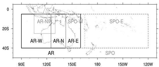
Figure 1.
Study area: the Australian region (AR) and the South Pacific Ocean region (SPO), and their sub-regions: northwestern AR (AR-NW), western AR (AR-W), northern AR (AR-N), eastern AR (AR-E), western SPO (SPO-W), and eastern SPO (SPO-E).
In this study, we use TC best track data for 45 seasons (1970/71 to 2014/15) from the Southern Hemisphere TC archive developed by the Australian Bureau of Meteorology in close collaboration with international partners: Regional Specialised Meteorological Centres (RSMCs) Nadi (Fiji) and La Reunion (France); and Tropical Cyclone Warning Centres (TCWCs) Brisbane, Darwin and Perth (Australia), and Wellington (New Zealand) [25]. To the best of our knowledge, the Southern Hemisphere TC data archive consists of the most accurate historical data records for occurrences of TCs in our study area for so-called “satellite era”, i.e., from the 1970s when satellite remote sensing data from geostationary and polar-orbiting meteorological satellites became available for operational use at meteorological services of Australia, New Zealand and Pacific Island countries [25,26,27]. Using these satellite remote sensing data, this study developed a novel methodology for improving accuracy of TC seasonal forecasting in the AR and the SPO region. The number of TCs for each season was obtained from the Southern Hemisphere TC archive via the Pacific Tropical Cyclone Data Portal of the Australian Bureau of Meteorology (http://www.bom.gov.au/cyclone/history/tracks/ (last assessed on 8 August 2022)). Note that in the Southern Hemisphere TC season coincides with the austral summer, typically starting in November and ending in April. As such, Southern Hemisphere TC season is described using two years, e.g., the season starting in 1970 and ending in 1971 is denoted as 1970/71.
TC intensity is usually defined in terms of maximum mean wind speed or minimum central pressure. To keep consistency with previous studies, the genesis of a TC is defined when a cyclonic system first attains a central pressure equal to or less than 995 hPa. Examining TC best track data in the Southern Hemisphere for “satellite era” (from the 1970s), it was recommended to classify a tropical system as a TC when this system attains minimum central pressure of 995 hPa or lower which corresponds to Category 1 on Australian tropical cyclone intensity scale [28]. In this study, the total number of tropical systems which attained TC intensity (995 hPa or lower) during TC season was used as a metric to calculate TC number for that season.
The Australian Bureau of Meteorology has operational responsibilities to issue TC seasonal outlooks for both AR and SPO regions and to provide Australians and the population of countries in the South Pacific Ocean with early warning advice about TC activity expected in the coming season [4,25]. These outlooks use the statistical relationships between TC numbers and two indicators: the SOI and the Niño3.4 sea surface temperature (SST) anomaly. These two indicators provide a measure of the atmospheric and oceanic state, respectively, of ENSO. Over the entire AR (S to S, E to E), this statistical relationship has proven to be highly accurate, or a skilful way to forecast TC activity. However, across the sub-regions this relationship, and thus forecast skill, can vary. Some regions have much higher forecast skill than others. The North-western sub-region (S to S, E to E) has good skill, while the Western (S to S, E to E) and Eastern (S to S, E to E) regions both have low skill and the Northern region (S to S, E to E) has very low skill (http://www.bom.gov.au/climate/cyclones/australia/#tabs=Further-information; accessed on 13 November 2022). The statistical model used for the SPO region outlook has a high level of accuracy predicting cyclone numbers in the western sub-region (S to S, E to E), but a very low level of accuracy for the eastern sub-region (S to S, E to W) (http://www.bom.gov.au/climate/cyclones/south-pacific/#tabs=Further-information; accessed on 13 November 2022). Low forecasting skill in sub-regions of the AR and the SPO region is identified as a deficiency of currently employed statistical TC forecasting methods. In this study, we attempt to improve statistical methodology for TC seasonal forecasting in the AR and the SPO region by selecting and averaging models via Metropolis–Gibbs sampling. There is an overlap between the two areas under investigation. This overlap is considered in this study; if a TC is recorded in both AR and SPO regions, we include it in our analysis for both areas.
To summarise, the focus of our study is on finding those climate indices which can significantly improve skill of TC seasonal forecasting in the AR and the SPO regions.
2.2. Model Covariates
Relationships between TC inter-annual variability in the regions of the Southern Hemisphere and key climate drivers – ENSO and IOD – were examined in [4,13,19,21,29]. These earlier studies have demonstrated that in the South Pacific Ocean TCs tend to form more towards the north-east of the region in El Niño years compared with La Niña years. In the south-west Indian Ocean, during positive (negative) phase of the IOD TC genesis is enhanced (suppressed) over the western (south-eastern) equatorial Indian Ocean. The results of [20,29] demonstrate that warm SSTs, enhanced atmospheric convection, increased relative humidity and reduced vertical wind shear are critical components in determining areas favourable for TC genesis in the Southern Hemisphere.
In the AR and the SPO region which are two regions under investigation in this study, ENSO significantly affected not only TC spatial distribution but also total annual number of TCs. In La Niña years, on average 10.3 TCs affected the AR while in El Niño years its average annual number was reduced to 8.2. In the SPO region, an increase in TC activity was observed in El Niño years (9.1 TCs on average) and a decrease in La Niña years (6.9 TCs on average) [4]. This modulation of TC activity by ENSO is based on changes in physical characteristics of atmospheric and oceanic environment. Warmer than normal SSTs, positive relative humidity anomalies and reduced vertical wind shear are found in the eastern (western) part of the SPO region during El Niño (La Niña) events, helping to explain the observed cyclogenesis.
As ENSO is a coupled ocean-atmosphere phenomenon, several indices which capture relative changes in both the atmospheric and oceanic environment potentially favourable for TC genesis over a large domain covering the equatorial central and eastern Pacific regions, were selected as potential variables to be examined in this study. These indices are described in Table 1 and considered in this analysis as the model covariates.

Table 1.
List of the observed climate variables, in August, September and October each year, in this study.
Variables Niño1+2 (hereafter, N12 ), Niño3 (N3), Niño3.4 (N34) and Niño4 (N4), as well as the El Niño Modoki Index (EMI) describe SST anomalies in various parts of the equatorial Pacific Ocean. Data for N12, N3, N34, and N4 come from the National Climatic Data Center (NCDC) (www.ncdc.noaa.gov/data-access/marineocean-data/extended-reconstructed-sea-surface-temperature-ersst-v5; accessed on 13 November 2022). Data for EMI come from the Japan Agency for Marine-Earth Science and Technology (JAMSTEC) (www.jamstec.go.jp/frsgc/research/d1/iod/DATA/emi.monthly.txt; accessed on 13 November 2022).
The Southern Oscillation Index (SOI) measures the ENSO-event-related atmospheric pressure differences. Specifically, SOI is a standardized index based on the observed mean sea level pressure (MSLP) differences between Tahiti and Darwin. Data for SOI, Tahiti MSLP, and Darwin MSLP were obtained from the Bureau of Meteorology (http://www.bom.gov.au/clim-ate/current/soi2.shtml; accessed on 13 November 2022).
Similar to the ENSO, the IOD is a coupled ocean-atmosphere phenomenon in the Indian Ocean. A positive IOD event is characterised by warmer than average SSTs in the western equatorial Indian Ocean and cooler than average SSTs in the south-eastern equatorial Indian Ocean. Typically, SSTs in the north Australian–Indonesian region and in the Coral Sea are also cooler than average during a positive IOD event. Associated with a westward shift of warmer ocean waters, the area of increased convection also shifts from the eastern to the western equatorial Indian Ocean. These coupled ocean–atmosphere changes during a positive IOD mode bring less favourable conditions for TC genesis to the AR and the western SPO region. On the other hand, during a negative IOD event, warmer than average SSTs over the south-eastern equatorial Indian Ocean, the Australian–Indonesian region and the Coral Sea lead to increased atmospheric convection over these regions and an associated increase in mid-tropospheric relative humidity creating a favourable environment for enhanced tropical cyclogenesis over this area. These relative changes in the oceanic and atmospheric environment associated with negative and positive phases of the IOD which impact on TC activity suggest that the Dipole Mode Index (DMI) which describes IOD’s status could be one of the key predictors for statistical models.
The DMI describes SST gradient between the western equatorial Indian Ocean (E–E and S–N) and the southeastern equatorial Indian Ocean (E–E and S–N). In this study, DMI, DMI West and DMI East indices which describe IOD’s state were selected as potential variables to be examined. Data for DMI, DMI West and DMI East were obtained from NOAA’s Physical Sciences Laboratory (PSL) (https://psl.noaa.gov/gcos_wgsp/Timeseries/DMI/; accessed on 13 November 2022).
The Quasi-Biennial oscillation (QBO) is characterized by downward propagating alternating easterly and westerly winds in the equatorial lower stratosphere with a period of approximately 28 months. Although the QBO is a stratospheric phenomenon, it has been linked to changes in many aspects of tropical convection, including variations in TC frequency and tracks in the Atlantic basin [30,31]. Moreover, QBO and ENSO are found to have combined influence on TC activity over the North Atlantic Ocean [32]. The emerging relationship between the QBO and the Madden–Julian oscillation (MJO) has been recently found [33]. Besides dominating sub-seasonal variability of rainfall and surface winds across the Indo-Pacific warm pool, the MJO drives variations in TC activity [34,35] and so is an important source of sub-seasonal climate predictability. As a potential indicator of TC seasonal activity in the Southern Hemisphere, QBO was not previously evaluated, and it was included in this study to be examined. Data for QBO is obtained from the National Oceanic and Atmospheric Administration (NOAA) (https://psl.noaa.gov/data/correlation/qbo.data; accessed on 13 November 2022).
3. Methods
Traditional statistical method of TC seasonal forecasting uses a particular small set of specifically selected indices based on prior knowledge of the relationship between TC activity and key climate drivers (e.g., SOI and Niño3.4 in the Australian Bureau of Meteorology’s operational model). This means that this traditional model has not included in it all important climate variables influencing TC activity in the best way. Improved seasonal forecasting results would be obtained by an improved operational model. This paper concerns finding the most important climate variables influencing TC activity and using them to establish a better model for seasonal TC forecasting. Model evaluation and hindcast analysis late in Section 4 confirm that our new approach improves TC seasonal forecasting.
We achieve improved TC seasonal forecasting by a new variable selection and model averaging approach. Variable selection is performed on Poisson regression model space by our stochastic search algorithm MGRS. Model averaging integrates and accordingly improves the forecasting performance of a small number of optimal Poisson models determined from variable selection.
3.1. Poisson Regression Model
We use the Poisson regression model to predict the TC number in a coming season in each given region. The Poisson distribution, describing the response variable (i.e., TC number) in the model, is widely used to describe count data, especially for events that happen in a fixed period, such as tropical cyclone numbers/counts, cold spells or frequency of droughts ([36]). Log-linear regression for Poisson-distributed data is a popular model used to study the associations between TC counts and various climate index covariates and to forecast seasonal TC activities. We assume the response variable Y is the tropical cyclone count in each season from to , and follows a Poisson distribution , where is the mean of Y.
Let be a column vector of p covariates. Here covariates are used, containing the August, September and October observations preceding each TC season for all the climate variables listed in Table 1. The Poisson log-linear regression takes the following form to model the relationship between Y and :
where is the unknown coefficient vector. Normally the coefficient is estimated by the maximum likelihood method but a Bayesian approach can also be applied to estimate the posterior distribution of (see e.g., [11]).
By fitting the seasonal TC data in Section 2 to the Poisson regression model (1), we obtain an estimate of the mean of Y at each given : . This estimate is actually a forecast of seasonal TC count for the season following the one when is observed. Confidence interval for this forecast can be subsequently calculated based on the standard error of each .
3.2. Model Selection and Averaging
We proceed to present statistical and computational details underpinning model selection and averaging. Let be a binary vector. Define a subset of , denoted , as such that if and only if . Namely, the jth element of indicates whether the jth covariate is included in the underlying candidate Poisson regression model. The candidate model specified by or equivalently by , denoted by , is written as
where is a sub-vector of indexed by which can also be estimated by the maximal likelihood method. Let be the space of all candidate models:
Now we can use to represent the corresponding candidate model . By model selection we mean to find the best model or or in the candidate model space.
To evaluate the utility of a candidate model (2), the Akaike information criterion (AIC) ([37]) is a popular and widely used choice (e.g., [38]). It is efficient and intends to select a model having the smallest predictive mean square errors. That is, the model with the minimal AIC value will have the best prediction performance. However, AIC has a tendency of over-fitting, especially in cases with small samples. Recall that there are only 45 samples in the seasonal tropical cyclone data set in Section 2. This suggests an improvement to be made on AIC. One such improvement, called corrected AIC (AICc), is developed in [22] and is defined for each model as
where is the log likelihood for model evaluated at the maximal likelihood estimator , n is the sample size, and is the number of parameters included in the model .
Treating AICc as a function on the candidate model space , finding the best model is equivalent to finding the minimal value of . When p is small, it is feasible to apply an all subset selection procedure to calculate for every model . However, the number of candidate models grows with p exponentially, and it becomes infeasible to perform all subset selection even when p is moderately large. A step-wise selection method has been used to tackle the difficulty which, however, cannot guarantee the selection of the globally best model but a locally optimal model instead, see [39].
To address the aforementioned difficulties, in this paper we turn to consider computationally feasible stochastic search approaches which is capable of finding the globally best model with probability 1 in the limit. Specifically, we propose a stochastic search algorithm of Metropolis–Gibbs sampling with random scan, denoted by MGRS, for model selection from . This new algorithm is motivated by the Gibbs sampler variable selection method developed in [23] but improves the computing performance over the latter. We proceed to describe the new algorithm in the following.
Define a probability distribution on the candidate model space by
where is a normalization constant, and is a tuning parameter. Clearly it is difficult to directly calculate the normalization constant Z when is enormous. On the other hand, the conditional distribution for each is Bernoulli, which does not involve Z and has the probability of “success”:
where . Generating samples of from the joint distribution can be achieved by Gibbs sampling through generating all conditional distributions in sequence at random and progressively, . By [24], each conditional distribution can be generated, rather than directly, but by Metropolis acceptance sampling, resulting in the aforementioned MGRS Algorithm 1.
Four remarks for the Metropolis–Gibbs random scan algorithm MGRS are made here.
First, from the definition of the probability distribution , it is obvious that the best model with the minimal AICc value will have the largest probability.
Second, for the tuning parameter k, a large k will put more probabilities on the better models having relatively small AICc values and expedites the equilibrium of the generated Markov chain, while it tends to hold on to a local best model. The converse is true for small k. In practice, a pilot run of the algorithm is often needed to determine a plausible range for k. In the current seasonal TC forecasting study, we find it sufficient to set k between and 10.
Third, the permutation is used to harness random scan. That is, the order by which the components of are randomly and sequentially updated in each round is determined by the current permutation. This way the generated Markov chain will be recurrent and reversible, so that the globally best model can be selected with probability 1 in the limit.
Last, the Metropolis sampling used in updating each component in Gibbs sampler is in effect generating with a probability larger than the conditional probability of specified by the corresponding conditional distribution in the Gibbs sampler. This implies the resultant generated Markov chain will converge to the equilibrium faster than the one generated by using Gibbs sampler alone.
| Algorithm 1: Metropolis–Gibbs sampling with random scan (MGRS) |
|
Let be the generated Markov chain sequence. It can be shown that S is an irreducible and reversible Markov chain with its stationary distribution being , because satisfies the detailed balance condition, cf. [40].
Practically, we choose to use the I-chart method to determine whether the sample sequence S reaches equilibrium after taking a burn-in period ([41]). It is equivalent to checking whether the corresponding sequence of the AICc values has reached equilibrium. With this generated AICc sequence, we can plot a modified individual point control chart or I-chart to do the checking. Knowing that AICc is actually a function of the random variable which follows the probability distribution defined on , it can be easily proved that
for any . Using this result, the lower control limit of the I-chart can be set to be , the minimum of the AICc series. The upper control limit of the I-chart can be chosen to be , where , , and are, respectively, the sample variance, the sample mean, and the sample minimum of the second half of the AICc series.
The generated AICc sequence is always above the lower control limit. On the other hand, when this sequence reaches equilibrium and , , and are consistent estimates, there would be less than of the AICc sequence over the upper control limit. Therefore, we can claim that there is no significant statistical evidence that the AICc sequence, and accordingly the generated model sequence S, have not reached equilibrium. Consequently, we will treat the model sequence S as though they were generated from the probability distribution , and then perform model selection and model averaging based on S and the associated AICc sequence. The I-chart proposed here will be said to be created by a level rule. Usually we use a level 90% rule to create the I-chart, corresponding to setting b equal .
Suppose the n generated models have formed a Markov chain in equilibrium, which is also true for the sequence . It is easy to find a model , named the estimated optimal model, such that . Given a small positive integer s, it is also feasible to identify the top s models from , denoted , such that .
In addition to being used for finding the best models, and the associated AICc sequence can be used to rank the importance to the response Y of each covariate component of . The importance of each covariate is determined by the frequency of the event appearing in . This frequency gives a consistent estimate of the marginal probability of with respect to the probability distribution . The marginal distribution of with respect to is Bernoulli with the probability of “success”:
which is the probability of covariate being included in a model generated by the MGRS algorithm. Note that using covariate importance ranking for model selection is similar to Bayesian variable selection ([42]).
Let be the sub-chain of consisting of all the ith components of . Although may not be a Markov chain when , the sampling distribution of converges to the marginal distribution of with respect to , where the probability of “success” is estimated by
Now we can use to represent the importance of covariate regarding its effect to the response Y. The most important covariates in are therefore determined by those having the largest values among ’s. Specifically, we can identify those important covariates by a pre-specified threshold such that .
In cases where the top s models from do not have a clear-cut winner, model averaging may be a better approach to finding a new model having improved predicting performance. Recall the top s models that have their respective coefficient estimates as . We define an extended smooth-AICc weight for each model in by
When , the ’s become the Akaike weights used in [43], which are commonly used among the model averaging methods. Here we choose the same k value used in the MGRS algorithm. Then the Poisson averaged regression model is defined as
When the prediction is the goal, it is recommended to use the model averaging method rather than the best model strategy ([44]). Model (6) is obtained by a Gibbs sampling induced model averaging approach, and is thus named the GMA model.
3.3. Model Evaluation
The leave-one-out cross-validation (LOOCV) approach is adopted in [45] to evaluate the predicting performance of a particular model characterizing Australian seasonal rainfall. We follow the same approach here. Namely, each season in the data is treated as a single fold, and the prediction of TC count in each season is obtained based on the fitted model using the data in all other seasons.
The mean square error (MSE) and the forecast skill score (SS) of a forecasting scheme in climatology defined by [36] are used in this paper:
where is the standard deviation of the TC counts y, and is the mean square error of the climatology model.
4. Results
4.1. Model Selection
This section presents and discusses the results of model selection and variable selection from analyzing the seasonal TC frequency data in AR and SPO regions across 1970/71 to 2014/15 seasons by the proposed MGRS algorithm and also the widely used step-wise selection method. We denote by BEST the best Poisson regression model selected by MGRS, and by STEP the final Poisson regression model selected by the step-wise method. In implementing MGRS we set the tuning parameter , and generate a sequence of models which is shown to achieve the equilibrium.
Figure 2 presents the level 90% I-charts for the generated AICc sequence in the Australian and South Pacific ocean regions and sub-regions. There is no significant statistical evidence to suggest that the generated AICc sequence has not reached equilibrium.
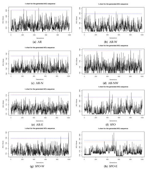
Figure 2.
The I-chart for the generated AICc sequence in each region. The blue dashed line is the upper control limit for generations 1:1000, and the red dotted line is for generations 1:500.
AICc values of the BEST models selected by MGRS from the generated model sequences for all regions are listed in Table 2, together with AICc values of the corresponding STEP models selected by the step-wise method. Table 2 shows that each model BEST always outperforms the corresponding model STEP by having a smaller AICc value.
Table 2.
The AICc values for the models STEP and BEST in each region.
For each model generated by MGRS for each region, we plot its frequency of occurrence in the generated model sequence against its AICc value. Results for all the generated models are displayed in Figure 3. Figure 3a–e shows that each BEST model has not only the smallest AICc value but also the highest sampling frequency within its respective AR sub-region. This conforms to what the probability distribution in (4) suggests.
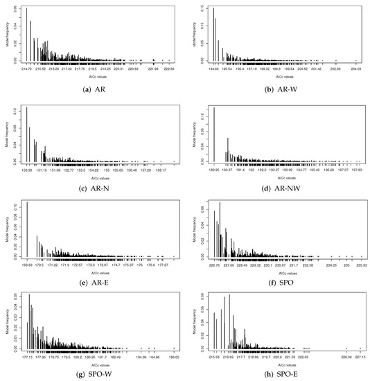
Figure 3.
Sampling frequency of each model present in the generated model sequence versus its AICc value for each sub-region.
Moreover, from both Table 2 and Figure 3 we see the model STEP selected by the step-wise method for most regions is far from being top ranked regarding the AICc value. For example, for sub-region AR-E, the model STEP has an AICc value equal to while we see is located in the middle of the AICc range from Figure 3e. The model BEST for AR-E has a much smaller AICc value equal to . This shows the step-wise model selection method does not work well in AR-E region and fails to find a model even close to the best model. Similar conclusions on the performance of the step-wise method can be drawn about the other AR sub-regions based on Figure 3a,c,d.
For the South Pacific Ocean region and sub-regions, Figure 3f–h displays the sampling frequencies for all generated models together with their AICc values. Unlike what is seen in the AR regions, both the BEST model and another model have the largest sampling frequency in SPO; the BEST model does not have the largest frequency in sub-region SPO-W; and only in SPO-E we see model BEST has the largest sampling frequency. This illustrates the uncertainty involved in model selection.
The marginal probability estimate given in (5) can be used to assess the importance of predictor in impacting the response variable y. Figure 4a–h display the 10 most important predictors with the associated 10 largest marginal probabilities in their impacting the seasonal TC frequency in each of AR and SPO sub-regions.
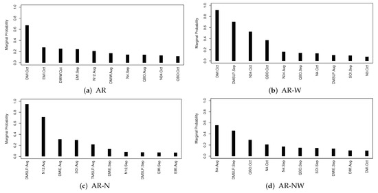

Figure 4.
The marginal probabilities for top ten predictors in each region.
For the AR region, DMI.Oct is the only one most important predictor with the marginal probability larger than , the next two EMI.Oct and DMIW.Oct are highly correlated. In summary, DMI and EMI are the two most important indices for seasonal TC forecasting in AR. For the AR-W sub-region, DMI.Oct is the most important and DMSLP.Sep is the second. Then we see DMI.Oct is the most important index in both AR and AR-W regions. For AR-N sub-region, DMSLP.Aug and N12.Aug are the top two important indices. However, for AR-NW and AR-E, no index has its marginal probability larger than , showing the limitation of the variable selection approach.
Figure 4f–h shows the top ten predictor indices with largest marginal probabilities for the SPO regions. For SPO we find EMI.Sep, DMI.Aug and TMSLP.Sep are the top three indices. For SPO-W we find N12.Sep and DMIW.Oct are the top two indices, while for SPO-E there are seven indices that have marginal probabilities greater than , including DMI.Oct having a marginal probability of nearly 1.
Finally, we can conclude DMI and EMI are among the most important indices for most regions. No other indices seem to be universally important across all sub-regions.
4.2. Hindcast Analysis
This section considers hindcast analysis of seasonal TC forecasting for AR and SPO and their sub-regions. Besides using the best models STEP and BEST selected by the step-wise method and the MGRS algorithm, we use two other models for assessing the performance of hindcast analysis. The first one is a weighted averaging Poisson model based on (6), denoted GMA, which averages the top log-linear regression models selected by MGRS to calculate the forecasting. The second one, denoted by X5VAR, is the Poisson regression model containing only the single index variable 5VAR proposed in [12] to calculate the forecasting.
Performance of the hindcast analysis by each of the aforementioned four models is evaluated by the three statistics nRMSE, MAE and SS defined in Section 3.3, which are computed using leave-one-out cross-validation (LOOCV). The results are summarized in Table 3, Table 4 and Table 5, where the best results for nRMSE and MAE are underlined.
Table 3.
nRMSE statistic for the hindcast analysis under LOOCV. The best result for each region is underlined.
Table 4.
MAE statistic for the hindcast analysis under LOOCV. The best result for each region is underlined.
Table 5.
Forecast skill score (SS) for the hindcast analysis under LOOCV.
Table 3 and Table 4 show that the model X5VAR has the worst performance among the four models in that it has the largest nRMSE and MAE and the smallest SS everywhere except for AR-NW with second largest MAE. Generally, it suggests the model X5VAR is not a good candidate for forecasting the seasonal TC activities, especially in SPO regions.
Regarding models STEP and BEST, their performances of hindcast analysis are close to each other. Table 3 and Table 4 show that model BEST performs better only in regions AR-W, AR-N, AR-E, SPO and SPO-W. However, the results from Section 4.1 show that model BEST has a smaller AICc value than model STEP in every region. Thus, model BEST does not always perform better than model STEP regarding the hindcast analysis under LOOCV.
For the model averaging approach, from Table 3 and Table 4, we see that the model GMA always has the minimal nRMSE and MAE, except in AR-NW where model STEP has the minimal MAE. From Table 5, model GMA improves much over the climatology model, especially in AR and AR-W, with SS values and , respectively. For the other regions, its SS values are over except in AR-NW. Moreover, for AR-NW, all models do not perform well with small SS values not more than .
In summary, the model GMA has the best performance of hindcast analysis on forecasting seasonal TC activities in AR and SPO regions. Figure 5, a visualization of the results in Table 5, displays the seasonal TC count observations and the hindcast values from models X5VAR and GMA under LOOCV. Among the four methods X5VAR, STEP, BEST and GMA, both Table 5 and Figure 5 show that X5VAR performs worst and GMA performs best across all regions.
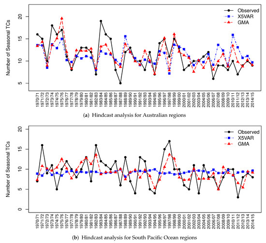
Figure 5.
The hindcast analysis results for AR and SPO regions.
5. Summary
In this paper, we have developed a Metropolis–Gibbs random scan algorithm MGRS for modelling and forecasting seasonal TC activities in AR and SPO regions and sub-regions. We have the following results:
- We have identified the most important climate indices impacting seasonal TC frequency in each region and find DMI and EMI are among the most important ones in most regions.
- Finding the best model with minimal AICc values is computationally feasible where the MGRS algorithm is superior to the step-wise method.
- The MGRS algorithm is used to find a small set of top models with relatively small AICc values which, by a Gibbs sampling induced approach of model averaging, forms a GMA model. The GMA model is shown to have improved the performance of hindcast analysis of seasonal TC frequency in all regions.
In general, our new method has significantly better performance than the traditional one. There are three possible reasons for this: (i) all potentially important covariates can be included for selection; (ii) MGRS is computationally feasible for finding the globally optimum solution; (iii) model averaging improves the forecast performance. The most important reason is believed to be (ii).
We also find that forecasting seasonal TC activities in the SPO regions is more challenging than in the AR regions, because in the former case there exist no clear-cut best models and it is difficult to identify the most important climate indices. Regarding the hindcast analysis performance, the model averaging approach is found superior to the model selection and variable selection approaches. However, it becomes more involved to interpret the influence of a climate index on seasonal TC activity for the model averaging approach. Finally, further research should be undertaken when more potential climate indices are discovered, especially in the SPO regions.
Author Contributions
Conceptualization, G.Q. and Y.K.; methodology, G.Q. and L.C.; software, L.C.; validation, G.Q., L.C. and Y.K.; formal analysis, G.Q. and L.C.; investigation, G.Q. and Y.K.; data curation, Y.K.; writing—original draft preparation, L.C.; writing—review and editing, G.Q. and Y.K.; visualization, L.C.; supervision, G.Q. and Y.K. All authors have read and agreed to the published version of the manuscript.
Funding
This research received no external funding.
Acknowledgments
We thank the four anonymous reviewers for valuable comments which helped us to improve quality of the manuscript and its presentation.
Conflicts of Interest
The authors declare no conflict of interest.
References
- Kuleshov, Y.; Spillman, C.; Wang, Y.; Charles, A.; deWit, R.; Shelton, K.; Jones, D.; Hendon, H.; Ganter, C.; Watkins, A.; et al. Seasonal prediction of climate extremes for the Pacific: Tropical cyclones and extreme ocean temperatures. J. Mar. Sci. Technol. 2012, 20, 675–683. [Google Scholar] [CrossRef]
- Kuleshov, Y.; McGree, S.; Jones, D.; Charles, A.; Cottrill, B.; Prakash, B.; Atalifo, T.; Nihmei, S.; Seuseu, F.L.S.K. Extreme weather and climate events and their impacts on island countries in the Western Pacific: Cyclones, floods and droughts. Atmos. Clim. Sci. 2014, 4, 803–818. [Google Scholar] [CrossRef]
- Do, C.; Kuleshov, Y. Multi-hazard Tropical Cyclone Risk Assessment for Australia. Nat. Hazards Earth Syst. Sci. Discuss. 2022, preprint. [Google Scholar] [CrossRef]
- Kuleshov, Y.; Gregory, P.; Watkins, A.B.; Fawcwtt, R.J.B. Tropical cyclone early warnings for the regions of the Southern Hemisphere: Strengthening resilience to tropical cyclones in small island developing states and least developed countries. Nat. Hazards 2020, 104, 1295–1313. [Google Scholar] [CrossRef]
- Nicholls, N. A possible method for predicting seasonal tropical cyclone activity in the Australian region. Mon. Weather Rev. 1979, 107, 1221–1224. [Google Scholar] [CrossRef]
- Nicholls, N. The Southern Oscillation, sea-surface-temperature, and interannual fluctuations in Australian tropical cyclone activity. J. Climatol. 1984, 4, 661–670. [Google Scholar] [CrossRef]
- Gray, W.M. Atlantic seasonal hurricane frequency. Part I: El Niño and 30-mb quasi biennial oscillation influences. Mon. Weather Rev. 1984, 112, 1649–1668. [Google Scholar] [CrossRef]
- Gray, W.M. Atlantic seasonal hurricane frequency. Part II: Forecasting its variability. Mon. Weather Rev. 1984, 112, 1669–1683. [Google Scholar] [CrossRef]
- Nicholls, N. Recent performance of a method for forecasting Australian seasonal tropical cyclone activity. Aust. Meteorol. Mag. 1992, 40, 105–110. [Google Scholar]
- McDonnell, K.A.; Holbrook, N.J. A Poisson regression model of tropical cyclogenesis for the Australian–southwest Pacific Ocean region. Weather Forecast. 2004, 19, 440–455. [Google Scholar] [CrossRef]
- Jagger, T.H.; Elsner, J.B. A consensus model for seasonal hurricane prediction. J. Clim. 2010, 23, 6090–6099. [Google Scholar] [CrossRef]
- Kuleshov, Y.; Qi, L.; Fawcett, R.; Jones, D. Improving preparedness to natural hazards: Tropical cyclone prediction for the Southern Hemisphere. In Advances in Geosciences: Volume 12: Ocean Science (OS); Gan, J., Ed.; World Scientific Publishing: Singapore, 2009; pp. 127–143. [Google Scholar] [CrossRef]
- Wijnands, J.; Qian, G.; Shelton, K.; Fawcett, R.; Chan, J.; Kuleshov, Y. Seasonal forecasting of tropical cyclone activity in the Australian and the South Pacific Ocean regions. Math. Clim. Weather Forecast. 2015, 1, 21–42. [Google Scholar] [CrossRef]
- Vitart, F.; Stockdale, T.N. Seasonal Forecasting of Tropical Storms Using Coupled GCM Integrations. Mon. Weather Rev. 2001, 129, 2521–2537. [Google Scholar] [CrossRef]
- Camargo, S.J.; Barnston, A.G. Experimental dynamical seasonal forecasts of tropical cyclone activity at IRI. Weather Forecast. 2009, 24, 472–491. [Google Scholar] [CrossRef]
- Johnson, S.J.; Stockdale, T.N.; Ferranti, L.; Balmaseda, M.A.; Molteni, F.; Magnusson, L.; Tietsche, S.; Decremer, D.; Weisheimer, A.; Balsamo, G.; et al. SEAS5: The new ECMWF seasonal forecast system. Geosci. Model Dev. 2019, 12, 1087–1117. [Google Scholar] [CrossRef]
- Vecchi, G.; Zhao, M.; Wang, H.; Villarini, G.; Rosati, A.; Kumar, A.; Held, I.; Gudgel, G. Statistical-dynamical predictions of seasonal North Atlantic hurricane activity. Mon. Weather. Rev. 2011, 139, 1070–1082. [Google Scholar] [CrossRef]
- Klotzbach, P.; Blake, E.; Camp, J.; Caron, L.; Chan, L.C.J.; Kang, N.; Kuleshov, Y.; Lee, S.; Murakami, H.; Saunders, M.; et al. Seasonal Tropical Cyclone Forecasting. Trop. Cyclone Res. Rev. 2019, 8, 134–149. [Google Scholar] [CrossRef]
- Kuleshov, Y.; Qi, L.; Fawcett, R.; Jones, D. On tropical cyclone activity in the Southern Hemisphere: Trends and the ENSO connection. Geophys. Res. Lett. 2008, 35. [Google Scholar] [CrossRef]
- Kuleshov, Y.; Chane Ming, F.; Qi, L.; Chouaibou, I.; Hoareau, C.; Roux, F. Tropical cyclone genesis in the Southern Hemisphere and its relationship with the ENSO. Ann. Geophys. 2009, 27, 2523–2538. [Google Scholar] [CrossRef]
- Wijnands, J.S.; Qian, G.; Kuleshov, Y. Variable selection for tropical cyclogenesis predictive modeling. Mon. Weather Rev. 2016, 144, 4605–4619. [Google Scholar] [CrossRef]
- Hurvich, C.M.; Tsai, C.L. Regression and time series model selection in small samples. Biometrika 1989, 76, 297–307. [Google Scholar] [CrossRef]
- Qian, G.; Field, C. Using MCMC for logistic regression model selection involving large number of candidate models. In Monte Carlo and Quasi-Monte Carlo Methods 2000; Springer: Berlin/Heidelberg, Germany, 2002; pp. 460–474. [Google Scholar]
- Liu, J.S. Metropolized Gibbs Sampler: An Improvement; Technical Report; Department of Statistics, Stanford University: Stanford, CA, USA, 1996. [Google Scholar]
- Kuleshov, Y. Climate Change and Southern Hemisphere Tropical Cyclones International Initiative: Twenty Years of Successful Regional Cooperation. In Climate Change, Hazards and Adaptation Options: Handling the Impacts of a Changing Climate; Leal Filho, W., Nagy, G.J., Borga, M., Chávez Muñoz, P.D., Magnuszewski, A., Eds.; Springer International Publishing: Cham, Swizerland, 2020; pp. 411–439. [Google Scholar] [CrossRef]
- Dowdy, A.; Kuleshov, Y. An analysis of tropical cyclone occurrence in the Southern Hemisphere derived from a new satellite-era dataset. Int. J. Remote Sens. 2012, 33, 7382–7397. [Google Scholar] [CrossRef]
- Broomhall, M.; Berzins, B.; Grant, I.; Majewski, L.; Willmott, M.; Burton, A.; Paterson, L.; Santos, B.; Jones, D.; Kuleshov, Y. Investigating the Australian Bureau of Meteorology GMS Satellite Archive for use in Tropical Cyclone Reanalysis. Aust. Meteorol. Oceanogr. J. 2014, 64, 167–182. [Google Scholar] [CrossRef]
- Kuleshov, Y.; Fawcett, R.; Qi, L.; Trewin, B.; Jones, D.; McBride, J.; Ramsay, H. Trends in tropical cyclones in the South Indian Ocean and the South Pacific Ocean. J. Geophys. Res. Atmos. 2010, 115, D01101. [Google Scholar] [CrossRef]
- Gray, W.M. Environmental influences on tropical cyclones. Aust. Meteorol. Mag. 1988, 36, 127–139. [Google Scholar]
- Gray, W.M.; Landsea, C.W.; Mielke, P.W.J.; Berry, K.J. Predicting Atlantic basin tropical cyclone activity by 1 June. Weather. Forecast. 1994, 9, 103–115. [Google Scholar] [CrossRef]
- Camargo, S.J.; Sobel, A. Revisiting the influence of the quasi-biennial oscillation on tropical cyclone activity. J. Clim. 2010, 23, 5810–5825. [Google Scholar] [CrossRef]
- Jaramillo, A.; Dominguez, C.; Raga, G.; Quintanar, A.I. The combined QBO and ENSO influence on tropical cyclone activity over the North Atlantic Ocean. Atmosphere 2021, 12, 1588. [Google Scholar] [CrossRef]
- Klotzbach, P.; Abhik, S.; Hendon, H.; Bell, M.; Lucas, C.; Marshall, A.; Oliver, E. On the emerging relationship between the stratospheric Quasi-Biennial oscillation and the Madden-Julian oscillation. Sci. Rep. 2019, 9, 2981. [Google Scholar] [CrossRef]
- Klotzbach, P.J. The Madden-Julian oscillation’s impacts on worldwide tropical cyclone activity. J. Clim. 2014, 27, 2317–2330. [Google Scholar] [CrossRef]
- Camp, J.; Wheeler, M.; Hendon, H.; Gregory, P.; Marshall, A.; Tory, K.; Watkins, A.; MacLachlan, C.; Kuleshov, Y. Skilful multiweek tropical cyclone prediction in ACCESS-S1 and the role of the MJO. Q. J. R. Meteorol. Soc. 2018, 144, 1337–1351. [Google Scholar] [CrossRef]
- Wilks, D.S. Statistical Methods in the Atmospheric Sciences; Academic Press: Cambridge, MA, USA, 2011; Volume 100. [Google Scholar]
- Akaike, H. A new look at the statistical model identification. IEEE Trans. Autom. Control 1974, 19, 716–723. [Google Scholar] [CrossRef]
- Magee, A.D.; Lorrey, A.M.; Kiem, A.S.; Colyvas, K. A new island-scale tropical cyclone outlook for southwest Pacific nations and territories. Sci. Rep. 2020, 10, 1–13. [Google Scholar] [CrossRef]
- Miller, A.J. Selection of subsets of regression variables. J. R. Stat. Soc. Ser. A 1984, 147, 389–410. [Google Scholar] [CrossRef]
- Robert, C.P.; Casella, G. Monte Carlo Statistical Methods; Springer: Berlin/Heidelberg, Germany, 2004; Volume 2. [Google Scholar]
- Qian, G.; Zhao, X. On time series model selection involving many candidate ARMA models. Comput. Stat. Data Anal. 2007, 51, 6180–6196. [Google Scholar] [CrossRef]
- George, E.I.; McCulloch, R.E. Approaches for Bayesian variable selection. Stat. Sin. 1997, 7, 339–373. [Google Scholar]
- Buckland, S.T.; Burnham, K.P.; Augustin, N.H. Model selection: An integral part of inference. Biometrics 1997, 53, 603–618. [Google Scholar] [CrossRef]
- Burnham, K.P.; Anderson, D.R. Multimodel inference: Understanding AIC and BIC in model selection. Sociol. Methods Res. 2004, 33, 261–304. [Google Scholar] [CrossRef]
- Drosdowsky, W.; Chambers, L.E. Near-global sea surface temperature anomalies as predictors of Australian seasonal rainfall. J. Clim. 2001, 14, 1677–1687. [Google Scholar] [CrossRef]


Publisher’s Note: MDPI stays neutral with regard to jurisdictional claims in published maps and institutional affiliations. |
© 2022 by the authors. Licensee MDPI, Basel, Switzerland. This article is an open access article distributed under the terms and conditions of the Creative Commons Attribution (CC BY) license (https://creativecommons.org/licenses/by/4.0/).