Liquefied Natural Gas and Hydrogen Regasification Terminal Design through Neural Network Estimated Demand for the Canary Islands

Abstract

This publication explores how the existing synergies between conventional liquefied natural gas regasification and hydrogen hydrogenation and dehydrogenation processes can be exploited. Liquid Organic Hydrogen Carrier methodology has been analyzed for hydrogen processes from a thermodynamic point of view to propose an energy integration system to improve energy efficiency during hybridization periods. The proposed neural network can acceptably predict power demand using daily average temperature as a single predictor, with a mean relative error of 0.25%, while simulation results based on the estimated natural gas peak demand show that high-pressure compression is the most energy-demanding process in conventional liquefied natural gas regasification processes (with more than 98% of the total energy consumption). In such a scenario, exceeding energy from liquid organic hydrogen carrier processes have been used as a Rankine’s cycle input to produce both power for the high-pressure compressors and the liquefied natural gas heat exchangers, generating energy savings up to 77%. The designed terminal can securely process up to 158,036 kg/h of liquefied natural gas and 11,829 kg/h of hydrogen.

1. Introduction

Due to recent events, the security of energy supply has become a priority issue for most European countries: greater diversification of supply sources, the guarantee of not being dependent on a single supplier and the inflationary crisis resulting from high energy prices are becoming strategic questions for preserving the continent’s industrial competitiveness and social welfare.

All the above become even more palpable in territories that act as energy islands. Their little or non-existent interconnection capacity and the absence, in most cases, of energy resources originating in these territories mean that these regions tend to have more polluting electricity generation mixes.

Within this paradigm, natural gas and LNG (Liquefied Natural Gas) midstream infrastructures—mainly materialized in regasification terminals—emerge as technical solutions. These facilities can provide a very significant improvement in the probability of supply interruption, greater stability and operational ease of the electricity grid plus an environmental improvement of emissions by displacing the use of heavier fossil fuels. With a high degree of technological development, these facilities can store LNG at very low temperatures (−160 °C) and returning it to its gaseous state through the application of heat exchange processes, enabling it to be imported from LNG carriers and injected into the transmission network after the corresponding compression stages (Figure 1).

Moreover, hydrogen is becoming a renewable alternative with a significant role to play in replacing natural gas in energy systems, as the existing natural gas assets has great potential to be reused with this new energy vectors due to its evident synergies. Nevertheless, the introduction of hydrogen in this type of facility still presents numerous technological challenges (due to its extremely low liquefaction temperature) for which no clear solution has yet been found [1,2,3]: although there are certain methods based on thermodynamic cycles [4,5,6] that have led to the development of recent liquid hydrogen transport projects [7], most of them require the design of complex conversion reactors to take advantage of ortho-hydrogen and para-hydrogen thermal properties. To avoid the abovementioned complexity, this paper proposes a chemical liquefaction method based on the use of Liquid Organic Hydrogen Carriers (LOHCs) through hydrogenation and dehydrogenation stages.

These processes rely on an unsaturated organic chemical agent in liquid state that can chemically retain the hydrogen atoms thanks to saturation reactions. These systems allow to release hydrogen by carrying out the opposite chemical reaction (generally varying the conditions of pressure and temperature of the process). Due to this, the LOHC adds several advantages compared to traditional hydrogen liquefaction systems:

• They allow to store the hydrogen in normal liquid conditions, rather than in extremely heat-insulated tanks.
• They widely simplify the liquefaction processes for hydrogen applications.
• They do not need as many resources (for example liquid nitrogen in traditional cryogenic solutions) as other methods. This also implies a significant decrease in OPEX.

On the other hand, neural networks have been used to model complex variables in many engineering and other science fields since its conception [8]. Nevertheless, their use today is still far from being considered as a mainstream tool in most of the basic engineering stages, even though they constitute a widely proven solution that can correctly assist to improve project’s results.

In this publication, the design of a hybrid regasification plant (capable of jointly managing hydrogen and natural gas) is carried out through the basic engineering of the traditional process together with a hydrogen chemical-liquefaction system using LOHCs, performing an energy integration analysis between both stages to achieve an optimization of the plant operation. The selected location for the plant is the Canary Islands (a clear example of an energy island), whose energy demand has been previously modeled to establish a defined neural network architecture that is able to predict the long-term power demand considering the daily temperature of the territory. The results are used to calculate the LNG and hydrogen demand as a design basis to perform the sizing general calculations for all the proposed processes. For the sake of clarity, a block diagram including all abovementioned study stages can be observed in Figure 2.

2. Materials and Methods

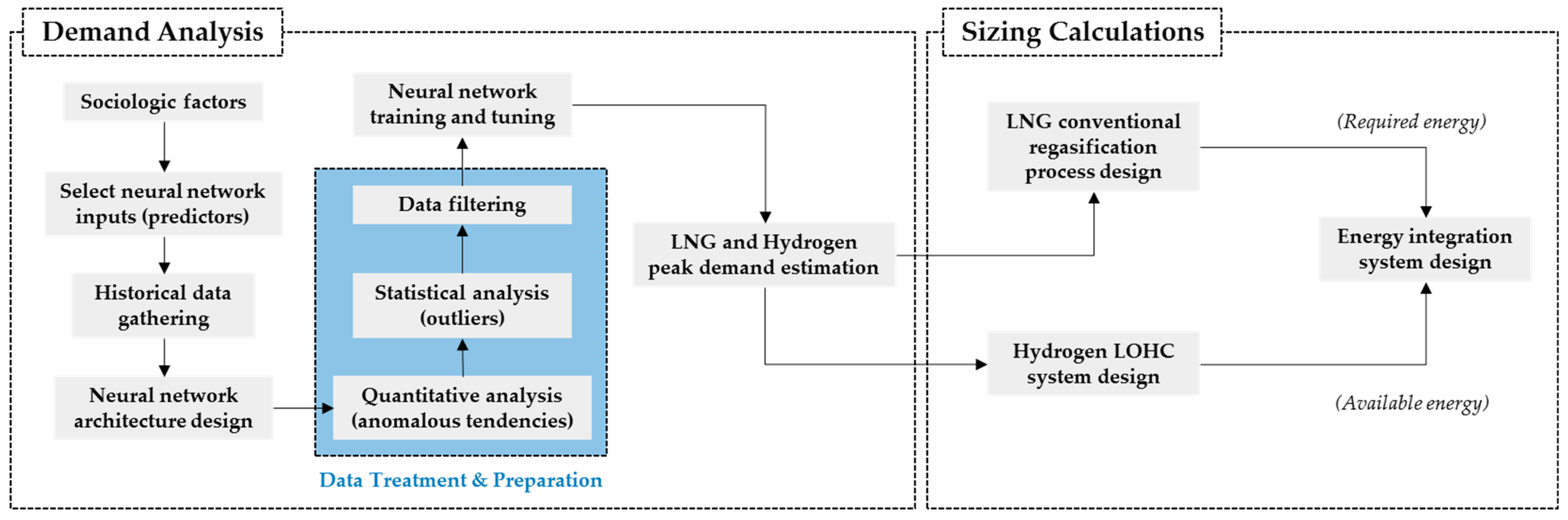
2.1. Demand Modeling

2.1.1. Sociologic Factors

From a general point of view, energy consumption is clearly affected by the number of customers that are located on a defined territory. For this reason, factors such as demographical tendencies should be considered whenever a demand scenario is being built, particularly when it comes to support predictive calculations results.

In this case, public data from Statistics Institute of the Canary Islands [9] are collected for the last 21 years including the total population and its rate of change, which will be used to validate from a qualitative perspective the results of the predicted peak power demand that will be used as a base to perform the sizing calculations.

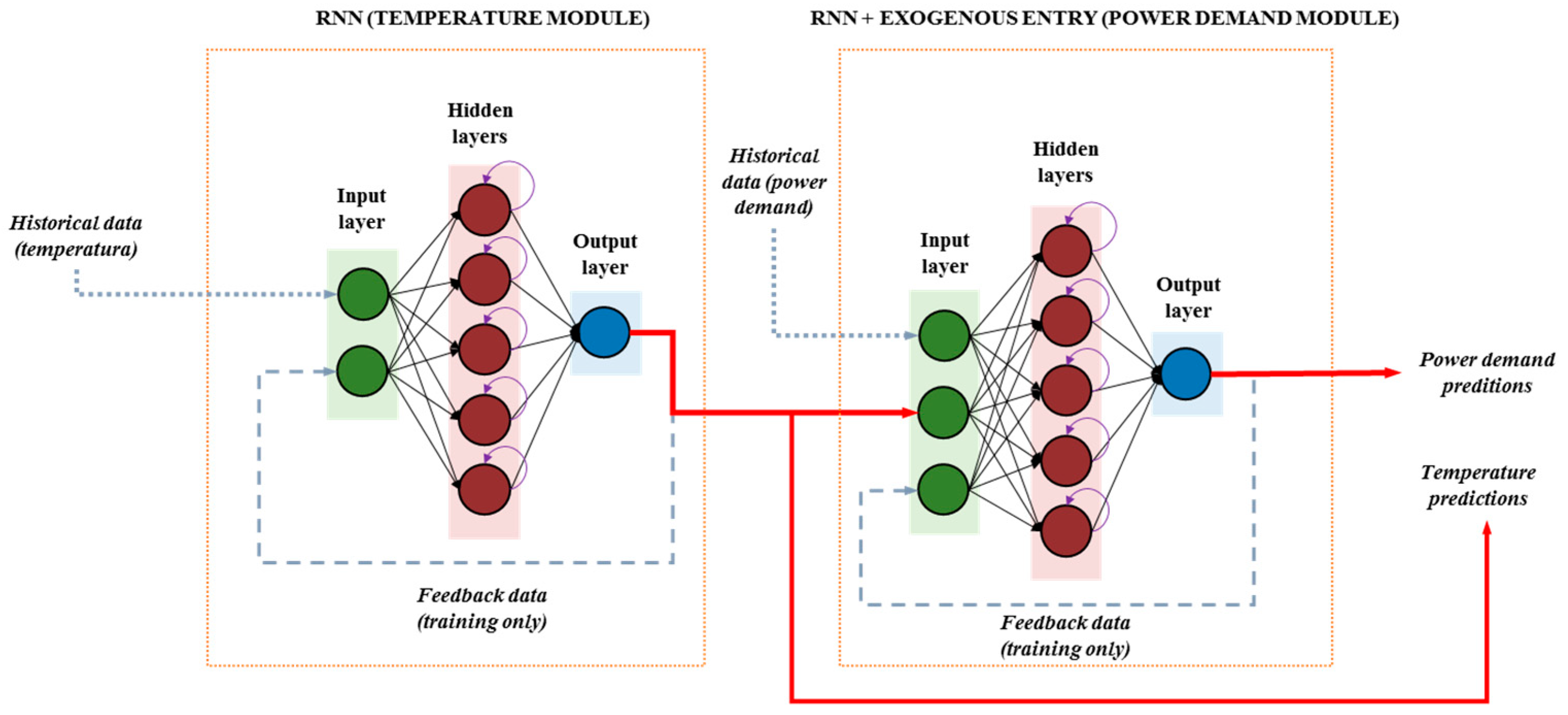
2.1.2. Neural Network Architecture and Inputs

A neural network is a connectionist model whose basic unit of transmission/reception of information and calculation is called a neuron. The main advantage that these systems add comparing to other common predictive methods (such as SARIMA models) lies in their autonomous ability to learn from historical data by applying certain algorithms that tend to reduce the difference between the desired output—the real historical data- and the actual output of the network, through the training process.

In this paper, and as the objective of the whole neural network is to precisely predict the peak power demand, only Recurrent Neural Networks (RNN) are going to be considered, as they give better results than other networks architectures when referring to time series analysis [10,11,12].

Even though these systems are a well-known and effective tool to predict complex systems using many variables, previous studies [12,13] show that acceptable results can be reached by using temperature data as a single predictor for energy demand forecasting.

On the other hand, it should not be ignored that both temperature and power demand are clear examples of self-regressive variables [14], which implies that their values as a generic nonlinear mathematical function y on a certain time t significantly depend on its previous values up to some past instant n:

y(t) = f(y(t − 1), y(t−2), …, y(t − n)),

(1)

With that being said, the optimal neural network model for this kind of applications must be able to group the two abovementioned principles while providing a statistically precise forecast. For that reason, the proposed architecture concatenates two different neural networks that act as independent modules, as can be seen in Figure 3.

The first module acts as a nonlinear autoregressive neural network that predicts future values for temperature depending on the historical data, while the second uses those predicted values as an exogenous input for another nonlinear autoregressive neural network to calculate the future values of power demand.

This modular scheme adds some advantages when compared to conventional neural network designs:

• Due to the independency of the modules between each other, parameters such as the delay or the percentages of samples that are used for training, validation and testing processes could be different.
• Each of the designed neural networks could be easily reused for other applications, once correctly trained and tuned.
• More predictors and/or exogenous inputs could be added in the future without modifying drastically the original scheme if the performance starts to drop.
• The specified parameters for each module can be found in

  Table 1. Neural network architecture parameters.

  Neural Network Module	Training Algorithm	Delay (d)	Number of Neurons (n)
  Temperature	Levenberg–Marquardt	5	35
  Power demand	Bayesian regularization	5	30

  .

Namely for this study, the delay values represent the amount of equally spaced previous data values (depending on raw data frequency) that are considered to adjust values predicted by the neural network during the training process, while the number of neurons show the network’s processing power (higher values imply more time for training processes and may lead to overfitting phenomena in case that excessively less generalization in predictions is reached [15]).

2.1.3. Data Treatment and Preparation

As the training process requires a significant amount of historical data to correctly tune the neural network, values from Red Eléctrica de España (Spain’s Transmission System Operator for the power grid) [16] and meteorological data [17] have been gathered for the last 10 years, including total power demand per day for the Canary Islands grid and average daily temperature respectively, both on a daily basis.

Firstly, a qualitative analysis of the conditions in which data occurred must be conducted, meaning that if some periods are under certain constrictions that are not likely going to happen in the future they must not be considered, just to protect the network of learn from unrepresentative data. Namely in this case, two different periods have been identified that can lead to a non-convergence loop during the training process:

• The significant decrease that weekends or festivities causes on power demand.
• The outbreak and subsequent restrictions of COVID-19 during the first half of 2020, which also affected drastically the power demand, eventually worsening the correlation between temperature and power demand itself.

Due to the abovementioned reasoning, from all the initially collected data pool, non-working days and data from dates ahead of 2020 are not considered.

Afterwards, a statistical analysis is carried out to determine from a quantitative point of view the outliers that remains basically to identify statistically anomalous data once raw data are free from long-term periods with externally affected causes. For this study, the application of a Tukey test [18] is proposed for its reliability with significantly long datasets and its great versatility to code in most of programming language. This test is essentially based on calculating the quartiles of each input pool, discriminating data depending on the deviation that the value represents from the interquartile ranges considering that a certain data can be classified as an outlier if it meets one of the following conditions [19]:

Value < Q₁ − 3 · (Q₃ − Q₁) [for downward outliers],

(2)

Value < Q₃ + 3 · (Q₃ − Q₁) [for upside outliers],

(3)

This statistical analysis is performed for both historical datasets. However, as each of these data corresponds to a certain date, whenever an outlier is detected, its corresponding pair must be also not considered in order to maintain time-data coherence between temperature and power demand time series.

By this point, the application of a smoothing method is carried out to improve the response and convergence of the neural network. Even though there are numerous models available, the Savitzky–Golay filtering [20,21] algorithm is proposed as the optimal solution in this application for several reasons:

• It is a widely tested solution in data sets that present high rates of variation in short intervals of time. In consequence, this type of approach has applications in many fields, such as analytical chemistry or sensor electronics [21].
• It does not significantly alter the general shape of the processed signal.
• Implies that the filtered data must be discretely and equally time spaced.
• It is relatively easy to code through standard programming.

This filtering stage will basically identify those data that, although they are not statically anomalous, represent a significant disruption in the general tendencies (such as heat or cold waves in temperature data set) that may lead to unrealistically repeat those patterns in the calculated predictions. As the Savitzky–Golay approach generally maintains the critical points location, it will simply increase or decrease those just to get rid of stational micro-patterns that may not occur in the same date for future periods.

Lastly, it is also worth mentioning that the neural network training process uses a standard sampling fraction [22] distinguishing randomly between:

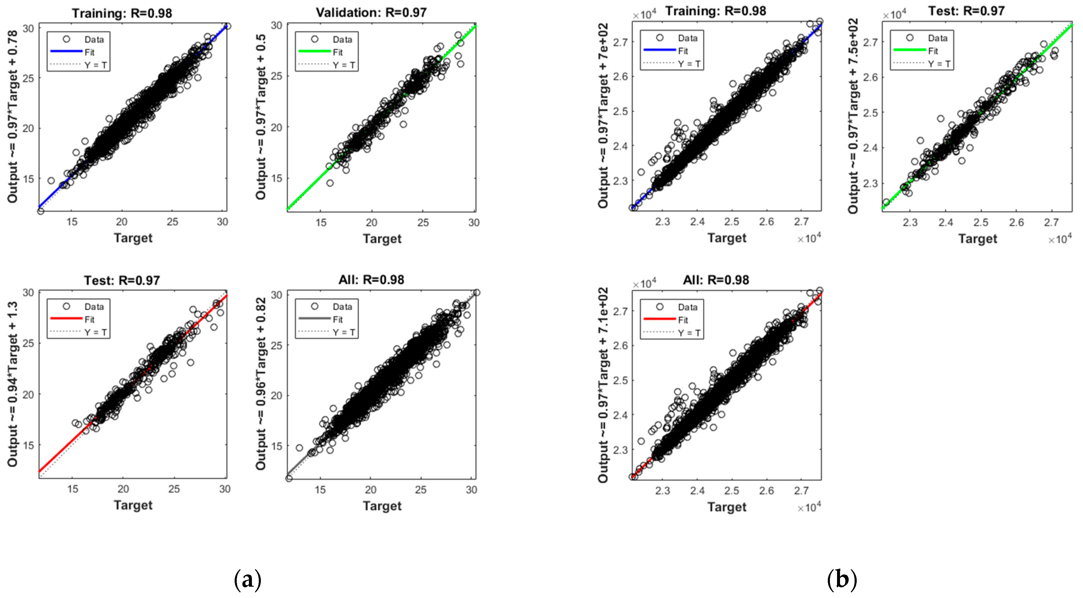
• Training samples (70% of each dataset): as the samples that are presented to the network during the whole training process. The tune of the whole architecture is adjusted according to its error regarding the real historical data.
• Validation samples (15% of each dataset): as the samples used to measure the network’s generalization. They are also used to halt the training process once the results stop improving.
• Testing samples (15% of each dataset): as the samples that are not used on the training and validations processes, and consequently, provide an independent measure of the network performance during and after the training process itself.

This distribution between the different types of samples has been chosen by the authors as the length of the input datasets is considered enough to provide an acceptable response. No further development has been carried out in this direction as overtraining phenomena (which occurs when the neural network is not able to recognize the underlying trends, resulting in poor generalization) need to be avoided as much as possible.

2.1.4. Considered Hypothesis for NG/LNG and Hydrogen Demand Estimation

Fossil fuels—mostly oil and its derivatives—are widely consumed on the Canary Islands nowadays due to its nature as an energy island [23]. In this context, the main idea of the terminal designed in this paper is to provide a reliable infrastructure to progressively replace the use of those heavy fuels by the combined use of hydrogen and natural gas (blending mixtures) to reduce the emissions of the territory, as environmental policies tighten to achieve increasingly ambitious climate goals in the upcoming years [24]. Therefore, it is assumed that the demand for both energy vectors will maintain a similar segmentation by sector as the demand that heavy fuels have nowadays [23,25]:

• Conventional demand: as the group that adds all residential and domestic consumption.
• Industrial and other services demand: in reference to touristic services (such as hotels, restaurants, small businesses, etc.) and industry (milk production, tobacco, refinery, etc.) of the islands.
• Power generation demand: grouping all the uses of natural gas for electricity production (mainly combined cycle plants).
• LNG and natural gas new uses: which include the potential demand due to the switching in certain sectors, such as maritime fuel in vessels, ships and ferries that transit the islands regularly.

Furthermore, and as the facility to be designed as a planned useful life of more than 35 years (2025 to at least 2060), a set of general long-term hypotheses must be established:

• The population amount, the distribution of consumers and their location within the islands will remain stable over time.
• Hydrogen as an energy vector will progressively replace the demand for gas and LNG from 2040, coexisting in a hybrid way with it until 2060, at which time the entire demand will be covered through gas of renewable origin.
• There will be no significant variation in the internal productive structure of the Canary Islands, as it will continue to be made up mainly of the services sector.
• If there were a drastic increase in power demand, its amount would be fully covered through renewable energies.

With that said, the peak demand for natural gas and hydrogen (D_NG,peak,year and D_H,peak,year, respectively) will be calculated at five years intervals depending on the peak power demand (D_{Power,peak,year}) forecasted by the neural network and a certain percentage (P_{NG,sector,year} and P_{NG,sector,year}, respectively) for each demand segment, by using the following expressions:

D_NG,peak,year = D_{Power,peak,year} · P_{NG,sector,year},

(4)

D_H,peak,year = D_{Power,peak,year} · P_{H,sector,year}

(5)

Percentages considered for each group of years and sectors for natural gas and hydrogen can be found in

Table 2. P_{NG,sector,year} values.

Year	Conventional	Industry and New Uses	Power Generation
2025	0.72%	7.97%	135.20% 1
2030	1.44%	23.06%	146.86% 1
2035	1.44%	30.09%	151.72% 1
2040	1.45%	30.37%	158.05% 1
2045	1.49%	25.22%	143.72% 1
2050	1.02%	17.88%	109.27% 1
2055	0.59%	11.36%	79.61%
2060	0.09%	4.18%	54.67%

¹ Note that p values above 100% for power generation implies an efficiency factor of 50% for combined cycle plants in days where thermal gap is very significant. The renewable capacity deployment in the near future at the Canary Islands do not affect these values, as p represents the peak consumption day (for example, a day with barely or non-existent wind resource).

and

Table 3. P_{H, sector, year} values.

Year	Conventional	Industry and New Uses	Power Generation
2045	0.00%	5.78%	17.60%
2050	0.44%	12.40%	48.30%
2055	0.89%	19.56%	81.27%
2060	1.37%	26.22%	103.53% 2

² As is the case for natural gas’ power generation segment, p values above 100% for power generation implies an efficiency factor of 50% for combined cycle plants that use hydrogen-ready turbines.

.

Standard properties [26] of natural gas and LNG used to perform conversion calculations are listed in

Table 4. Natural gas, LNG and hydrogen properties.

Component	Density (kg/m3)	Gross Calorific Value (kWh/Nm3)
Natural gas	0.69	11.63
LNG	431.07	- *
Hydrogen	0.09	3.08 **

* LNG’s GCV (Gross Calorific Value) is not considered, as the LNG mass flow will be calculated only using the relation between natural gas and LNG densities. ** Hydrogen’s GCV [27] considers a density of 0.089 kg/m³ and a Wobbe Index of 11.29 kWh/Nm³.

.

2.2. Sizing and Simulation

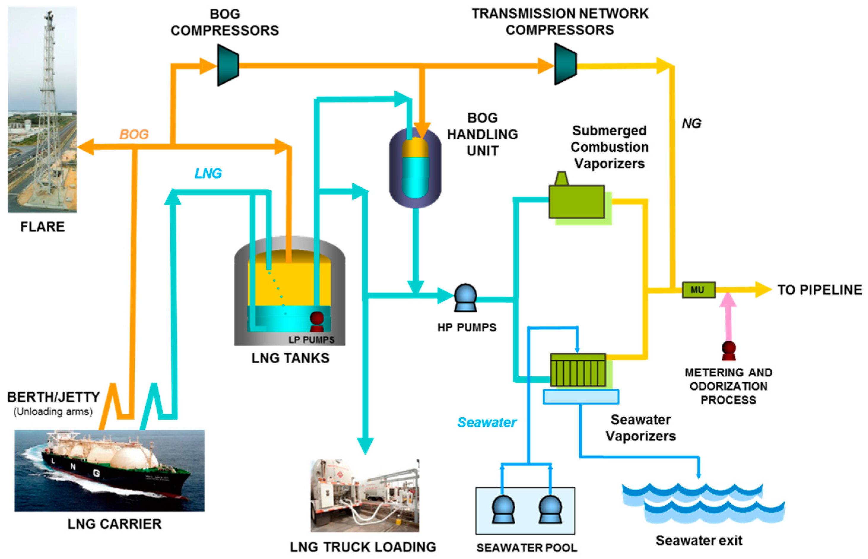
2.2.1. Regasification Processes

For the traditional regasification process (Figure 1), this paper proposes a simplified scheme in ASPEN HYSYS to size and simulate the main equipment of the facility [28,29], considering the following stages:

• Storage stage: as the part of the plant in charge of receiving the unloaded or reliquefied LNG and maintaining its temperature to avoid its involuntary evaporation (boil-off gas formation). It basically consists of the cryogenic tanks and the associated pressurization units (submerged LNG pumps).
• Liquefaction stage: referred to the part of the terminal responsible for liquefying BOG (Boil-Off Gas). It consists of open heat exchange units capable of withstanding very low temperatures and a small compressor.
• Regasification stage: associated with the entire process of heating the LNG coming from the storage and/or liquefaction stage, bringing together the heat exchange processes for the temperature increase and ensuring its correct vaporization. It consists of the heat exchange equipment using seawater as the hot fluid.
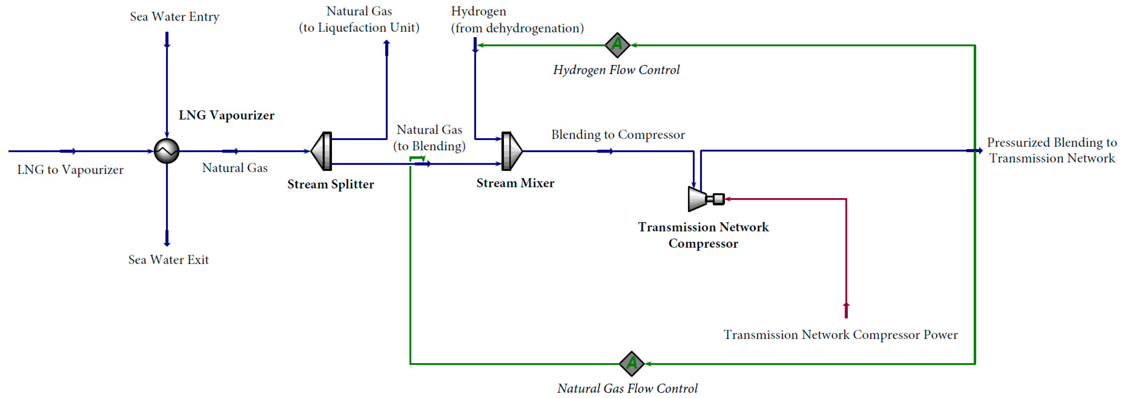
• Compression stage: to pressurize natural gas into transmission network. It basically consists of a group of high-pressure compressors.

With that said, the simulated PFD (Process Flow Diagram) model can be found in Figure 4 including certain particularities:

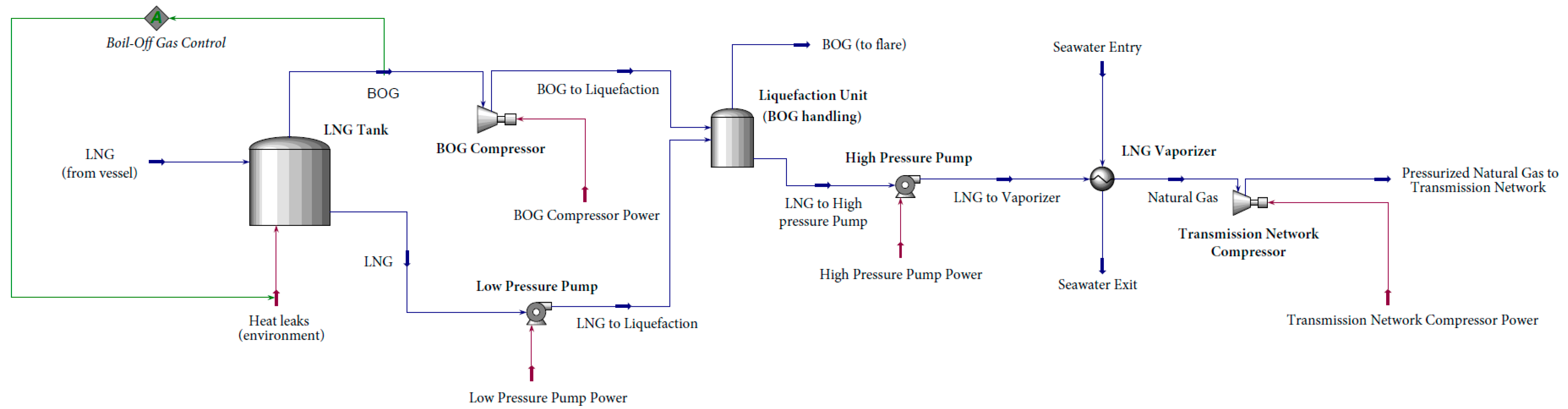
• HYSYS differentiate between material streams (mass flows, marked in blue in PFDs) and energy streams (energy flows, marked in red in PFDs). Note how an energy stream has been added to the storage stage just to represent the heat leak that the tanks suffer, producing the BOG by involuntarily vaporizing the LNG.
• Control streams (marked in green in PFDs) have been used to calculate the maximum limit of heat that the tanks can exchange with the environment to produce a defined amount of BOG (in terms of mass flows).
• The liquefaction unit is modeled as a tank unit as HYSYS do not have any specific system to simulate open heat exchangers. In practical terms, this means that BOG will be turned into LNG by simply getting in contact with the LNG withdrawn from the storage unit. Non-liquefied BOG will be directed to flare.

Regarding the specified parameters, the simulated model considers the following design requirements:

• The LNG and natural gas composition is assumed as 97.85% of pure methane (CH₄), 0.85% of diatomic nitrogen (N₂) and 1.3% of carbon dioxide (CO₂). Unloading LNG temperature and pressure are fixed at −164 °C and 0.875 bar, respectively.
• The storage unit dimensions must be able to store at least an amount of LNG equal to the peak regasification capacity of the facility working in full rate for 15 days, maximizing the security of supply [30].
• The maximum BOG rate allowed is defined as an 0.75% (on a mass per day basis) of the total LNG stored [31].
• The vaporizer design will be carried out by minimizing seawater consumption considering that seawater cannot be returned to the sea if its temperature is below 11 °C in the whole Spanish territory, as the minimum temperature allowed is 10 °C [32].
• The entry pressure of the transmission network is fixed at 60 bar [33], as it is considered a high-pressure network.
• The whole design will be resolved using Soave–Redlich–Kwong (SRK) equation-of-state [34,35,36].

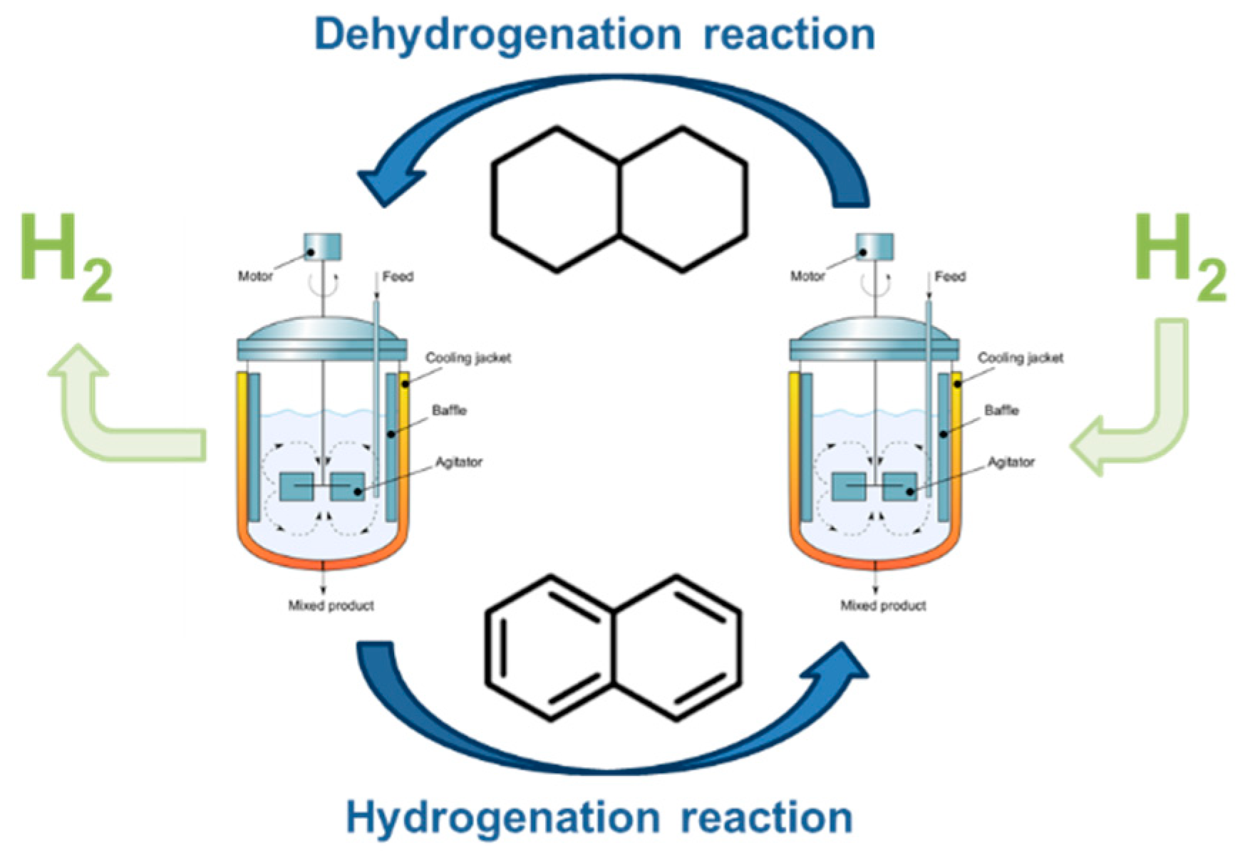
2.2.2. Hydrogen LOHC Hydrogenation and Dehydrogenation System

Hydrogen liquefaction processes had always supposed a technical challenge due to its low condensation temperature (approximately at −253 °C).

Although there are several significant lines of research about this methodology [37,38], there are already a considerable number of organic components available that can meet these needs in a very solvent way. In this case, the simulated process will use a naphthalene-decalin system as the LOHC for hydrogen chemical liquefaction, whose simplified process can be found in Figure 5.

Contrary to the LNG regasification conventional process, hydrogen’s LOHC processes will be modeled and resolved in ASPEN PLUS, as a more accurate thermodynamic solution is required, considering the following stages:

• LOHC saturation reaction: strongly exothermic by breaking the double bonds of the unsaturated LOHC to add hydrogen atoms to the resulting molecule (usually referred to as LOHC+).
• LOHC desaturation reaction: once desired, the LOHC+ formation reaction can be reversed by removing hydrogen from the saturated chain and forcing the appearance of the multiple bonds of the original LOHC molecule (strongly endothermic).
• LOHC recovery: after a considerable number of reaction cycles, it is advisable to replace all or part of the LOHC used in the system to prevent the occurrence of parasitic chemical reactions. This implies the existence of separation units that allow to effectively remove the LOHC from the gas hydrogen once the dehydrogenation reaction took place.

With that said, the simulated PFD model can be found in Figure 6 including the following particularities:

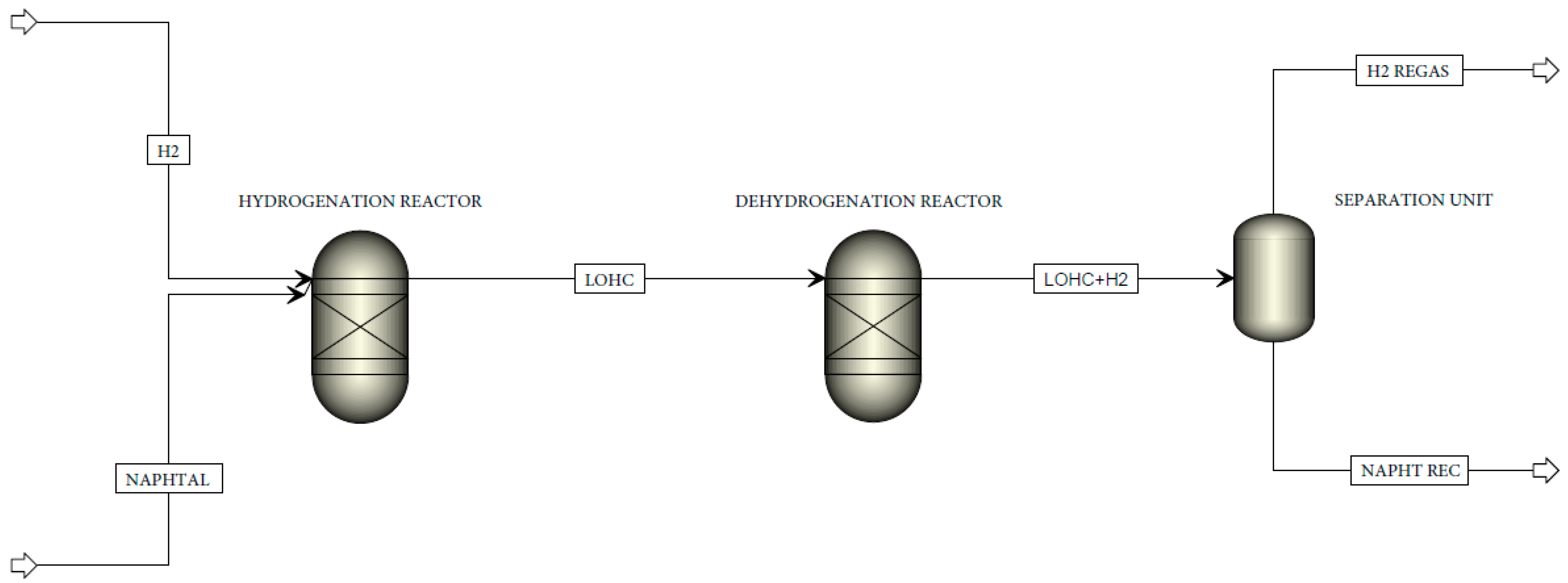
• ASPEN PLUS does not only resolve material streams (mass flows). Therefore, no energy streams are defined as energy requirements will be calculated once the simulation process solves the case.
• Both reactors’ units (hydrogenation and dehydrogenation) will use a Gibb’s free energy formation minimization algorithm to predict the LOHC conversion to saturated and unsaturated states.
• The separation unit will be modeled as a flash column, only being defined by temperature and pressure conditions to separate both fluid phases.

Regarding the specified parameters, the simulated model considers the following design requirements:

• Input streams are considered pure for both LOHC and hydrogen. Additionally, these streams are processed at 25 °C and 1 bar.
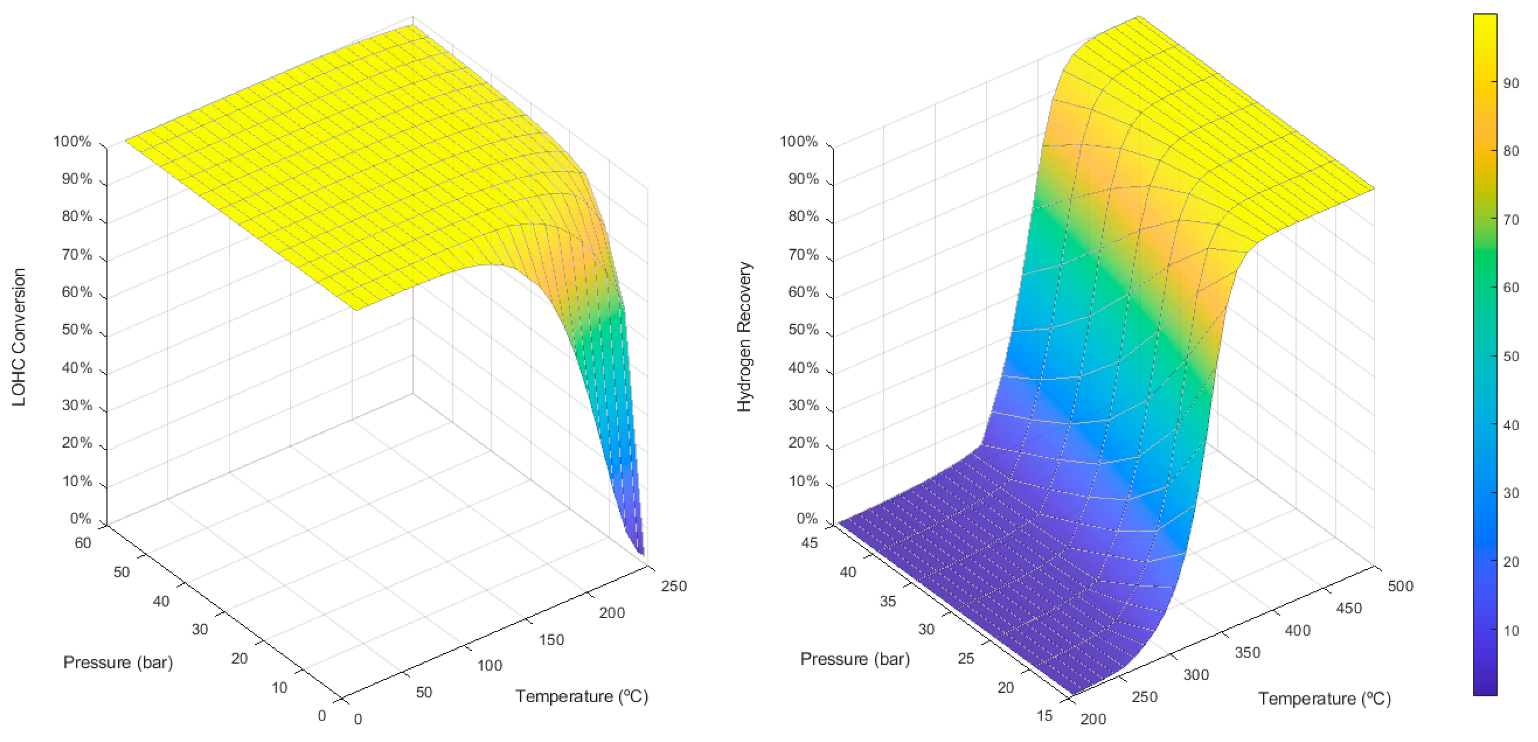
• A sensibility analysis will be carried out to optimize the reaction conditions (namely pressure and temperature) for both reactions.
• Conditions in separation unit are calculated to not vary the chemical composition of the gas and liquid phases that comes from the dehydrogenation reactor. Only physical separation between both phases is required.
• The whole design will be resolved using the Peng–Robinson equation of state, as it is the most widely used thermodynamic model [39,40] to predict liquid phases behavior.

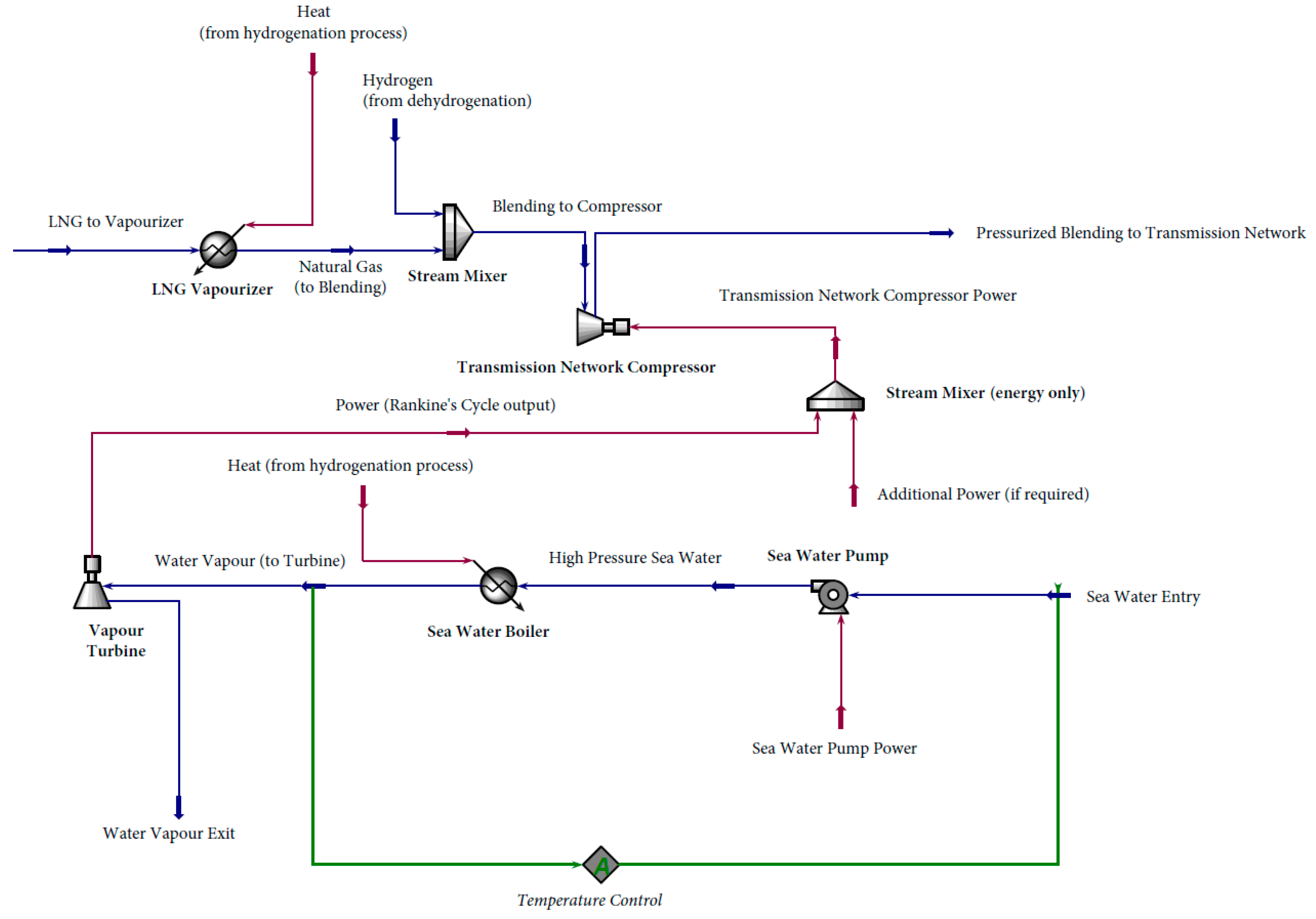
2.2.3. Energy Integration System

Once the hydrogen LOHC system have been fully designed, an energy integration analysis between the LNG regasification processes and the hydrogen organic reactions is carried out.

The main idea behind this study is based on achieving the greatest possible energy savings within the LNG regasification stage thanks, to a large extent, to the energy provided by the strong exothermic reaction produced by saturating the LOHC bonds in the hydrogenation reactor.

In this regard, the most energy demanding process must be identified, as it will be the one more suitable to apply energy efficiency measures. For most LNG regasification terminals, the highest energy consumption is at compression stages [41,42]. Due to this, a power demand analysis is proposed by modifying the PFD on Figure 4 by including a new stream material of pure hydrogen that is mixed with the regasified LNG until a specified molar fraction of hydrogen in the blending mixture is reached, as can be seen in Figure 7.

Once HYSYS resolve the proposed system, the available energy to be used on this compression process (E_available) can be estimated by adding the heat produced at hydrogenation (Q_hydro) reactor plus the amount of cooling needed to reach the temperature conditions at the separation (Q_separ) unit by using the following expression:

E_available = |Q_hydro| + |Q_separ|,

(6)

Despite the fact this may represent a significant quantity of available energy, it cannot be directly reused to power the compression stage as it must be converted to mechanical or electrical energy. To perform this energy conversion, this study proposes the addition of a simplified Rankine cycle, where the power turbine will be shaft-coupled with the transmission network compressor, providing as much energy as produced by the cycle directly to the compression stage (Figure 8).

Lastly, if there is still available energy, it can be used to reduce the seawater consumption during the LNG heat exchange stages (represented by the substitution of the seawater material streams for just one energy stream on LNG Vaporizer). Regarding the specified parameters, the simulated model considers the following design requirements:

• Seawater input stream is at 15 °C and 1 bar.
• One control stream is added to ensure that seawater does not surpass 600 °C at the turbine’s entry. Once this temperature is reached, the rest of the available heat will be used for LNG heat exchange energy savings.
• An extra energy stream is added to the one produced by the Rankine’s turbine just to solve the cases that more energy is required to pressurize the blending mixture.
• The whole design will be resolved using Soave–Redlich–Kwong equation of state, to maintain coherence between the results from the conventional LNG regasification processes results.

3. Results and Discussion

3.1. Demand Estimation

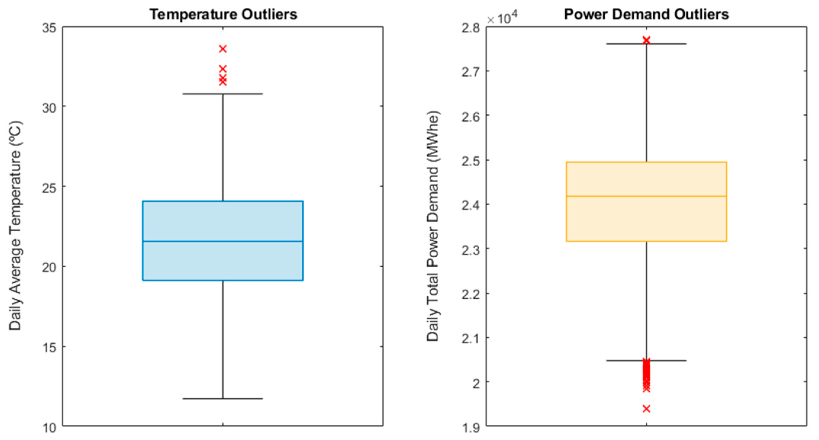
3.1.1. Data Outliers’ Determination

The outlier’s determination analysis (described by Tukey’s test equations previously mentioned) results are presented as standard box plots in Figure 9.

The median for each dataset is illustrated as the horizontal line inside the box, whose limits corresponds to Q₃ and Q₁ (in other words, the box defines the interquartile range). The whiskers, on the other hand, represent the Q₀ and Q₄, meaning the lowest and highest data point in the dataset, respectively, excluding any outliers. All data that do not fit into those limits are noted with a red cross and qualified as an outlier.

The test results show that only four values of the whole temperature dataset represent a statistically anomalous behavior, all of them being considered as upside outliers. For the power demand data series, a total of 38 values are identified, labeling 4 of them as upside outliers and the other 34 as downside outliers.

As has already been explained, to maintain time coherence between both temperature and power demand datasets, all identified outliers from one data series and its corresponding pair (date-coupled values) are not considered in further stages.

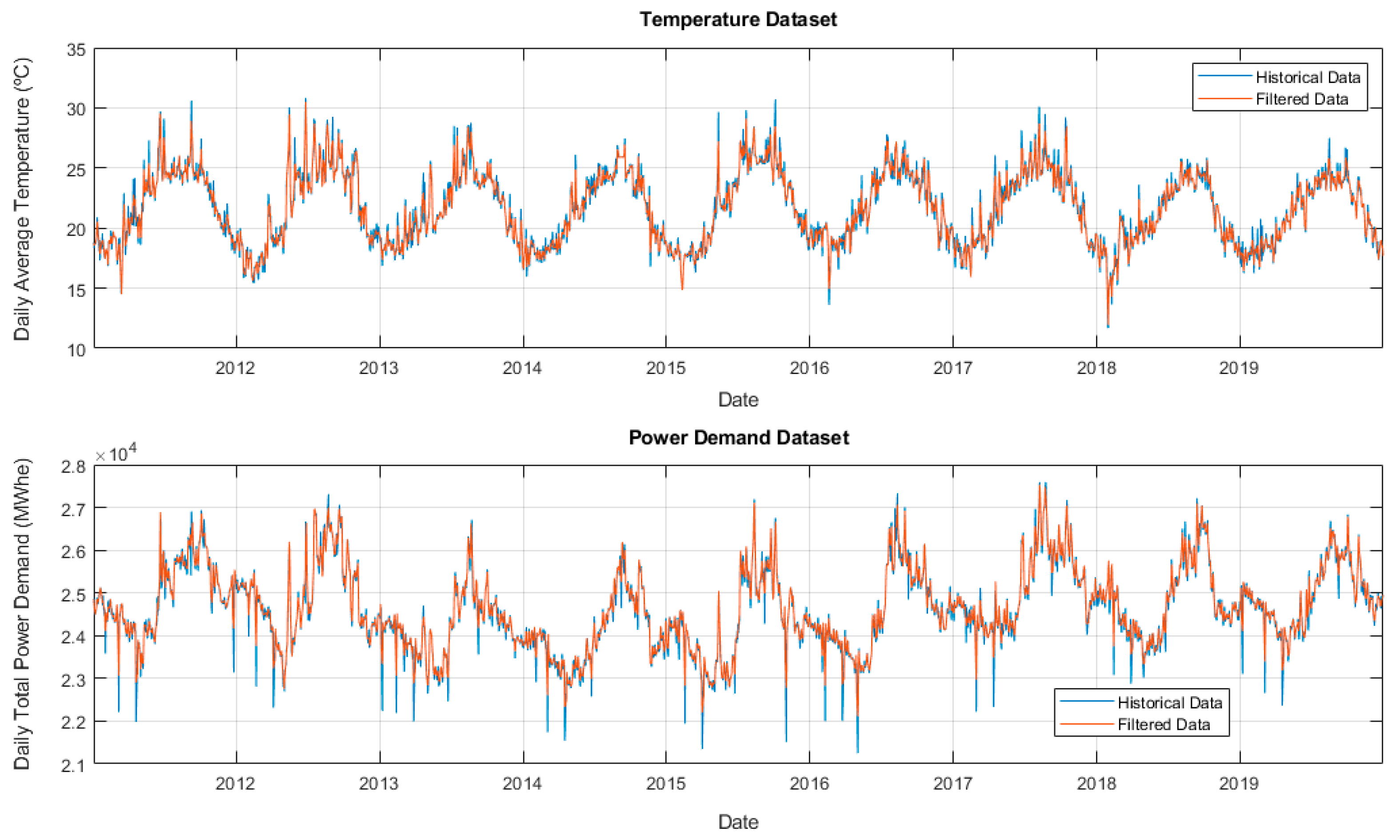
3.1.2. Filtering Process

The Savitzky–Golay filtering process results are displayed in Figure 10 individually for each dataset.

As expected, the filtering process does not significantly modify the general shape of both series, maintaining an acceptable location of turning points. Nevertheless, it is remarkable how power demand historical data show several minimum values that do not correspond with weekend periods or with the main festivities, which may be due to many reasons:

• Local festivities that have not been identified (as, for example, the Holy Week period that varies its dates of celebration each year).
• Conjunctural conditions to the Canary Islands energy system that influence the demand, such as for example national strike callings.
• Power shortages or energy distribution failures that may had occurred.

In any case, and even though the Savitzky–Golay approach allows to recognize these data as minimums, their values are generally increased to reduce their impact on the neural network training process. By correcting these minimums closer to the general range of values of the power demand data, the variance ratio of the filtered data is considerably reduced, and consequently, a better (and faster, in most of the cases) statistically acceptable accuracy during the neural network tune can be reached.

For the maximum values, the case is simply the opposite, as they are the most important values in which predictions must be based on. For this reason, the filter process firmly maintains most of the original historical data, adding minuscule corrections.

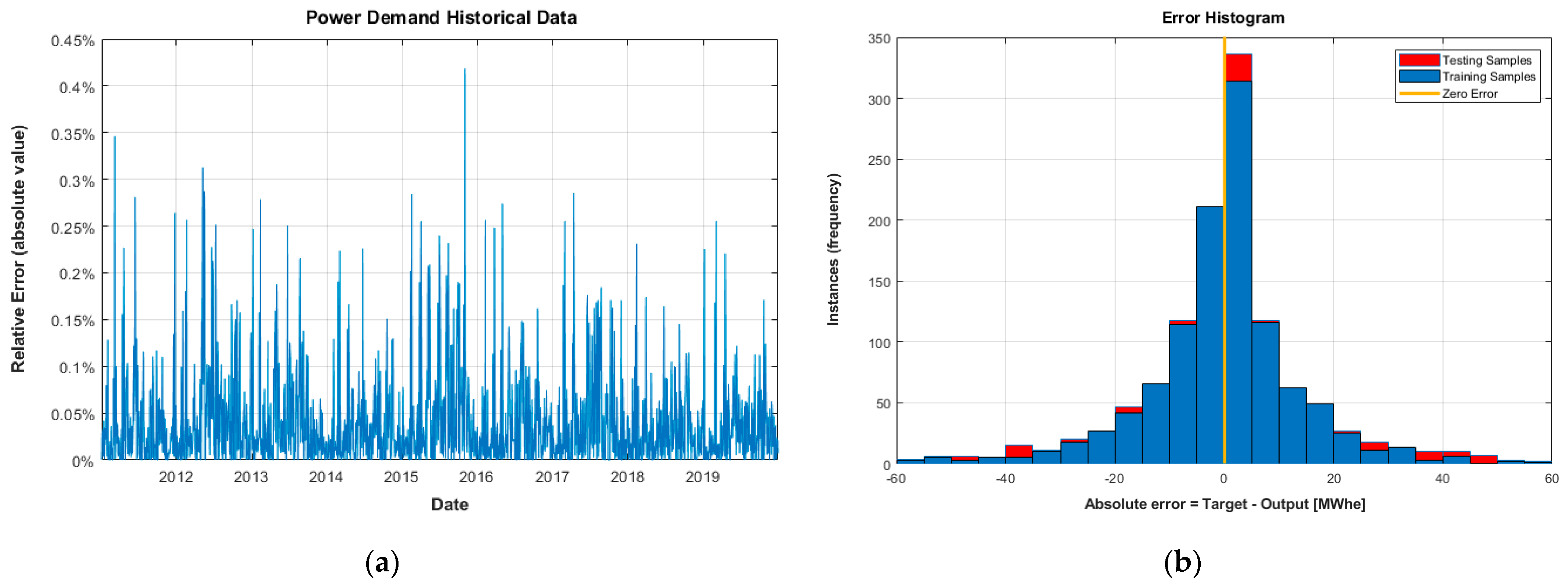
3.1.3. Neural Network Training Process

As the architecture parameters considered for each module is fixed as described previously, all that is left is to check that the whole system can reach enough accuracy regarding the historical data during a reasonable time of training. The main results of the process are collected in

Table 5. Neural network’s training algorithm performance.

Neural Network Module	Training Algorithm	Number of Iterations	Time of Training (s)	Average MSE (Training, Validation & Testing Samples) 3
Temperature	Levenberg–Marquardt	12	1	0.33 [°C]
Power Demand	Bayesian regularization	847	53	268.29 [MWhe] 4

³ The mean squared error (MSE) is usually used as the main risk function to calculate the performance of a neural network [43]. Values closer to zero means a perfect prediction in which the model can exactly predict the training data. ⁴ For the case of the power demand module, the average MSE calculations considered a value of 0 for validation samples because of the Bayesian regularization algorithm. The average MSE represents 1.08% of the average power demand historical data, which is considered an acceptable convergence.

.

As can be seen, the neural network reaches an acceptable solution in less than 1 min of training in the case of the power demand module. The significant differences between the number of iterations and the time of training for each module simply responds to the architecture: for the temperature module, the network must process only non-coupled values of the historical data, as there are no other inputs, while in the case of the power demand module the network must deal with the paired data by the exogenous entry. This could be corrected using lighter—in terms of computing power requirements—training algorithms for the power demand stage (such as for example the scaled conjugate gradient algorithm), generally implying worse quality of predictions. Regarding the MSE values, both are considered as good enough for the application that this paper proposes.

In addition, all samples are regressed individually (Figure 11) depending on whether it is easily proven that the random sampling methodology is working properly and there is not any group that presents a significant deviation in respect to the others. No anomalous tendencies were observed in this regard, so the sampling process is considered correct.

Lastly, absolute and relative errors for the historical data are calculated (Figure 12). The results shown a mean relative error of 0.039% and a highly zero-centered absolute error histogram with equally upside and downside distribution. The main contribution to the absolute error comes from the training samples (more than 80% of the instances), basically due to the higher percentage of the sampling distribution for this type.

Due to the abovementioned reasonings and results, the neural network is considered reliable enough to provide a trustworthy prediction to be used as a base for the design stage.

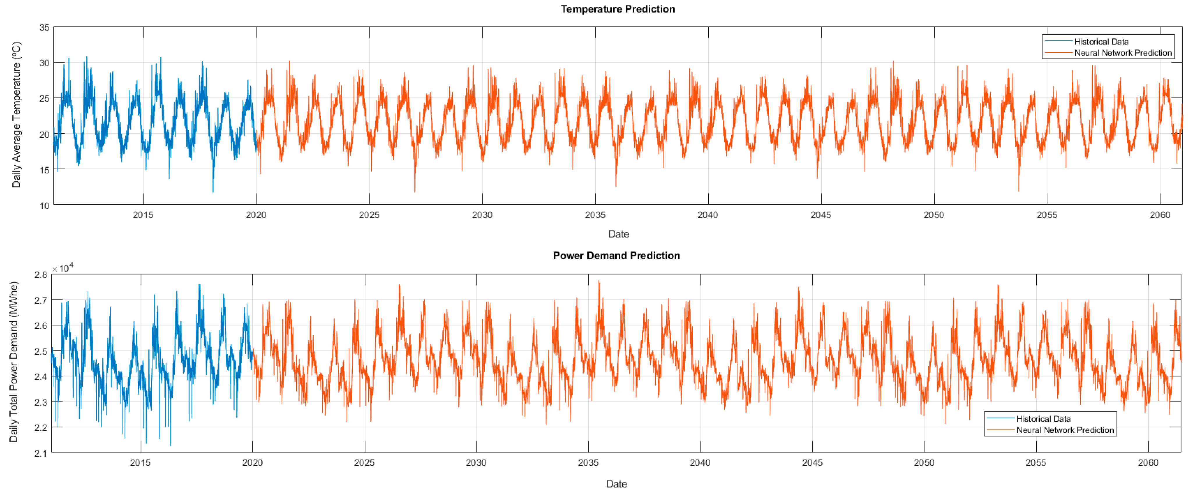
3.1.4. Power Demand Predictions

By the time neural network training process conclude, the whole system is set up to start predictive calculations. The given solution can be observed in Figure 13 for the years 2020 to first half of 2060.

The results showed a clear steadiness in both variables, which is considered as a reasonable outcome for many reasons:

• No increase in population is expected on the Canary Islands, as most of the territory is already being used (and a significant part of the area is environmentally protected) [44].
• Industrial expansion is barely expected, as their economic model is mainly based on tourism and vessel traffic in the main ports [45,46].
• The temperature is highly influenced by the thermal inertia of the ocean and, therefore, heat or cold waves are punctual phenomena [47].

With that being said, the peak power demand for five-year-long groups (starting with the predicted data at 2020) is listed in

Table 6. Peak power demand predicted by the neural network.

Year	Predicted Peak Power Demand (GWhe)
2025	27.59
2030	27.75
2035	27.75
2040	27.49
2045	26.93
2050	27.57
2055	27.01
2060	27.47

.

3.1.5. NG/LNG and Hydrogen Peak Demand

Once the power demand prediction has been obtained, and by applying the equations and percentages defined for each year that has been previously described, the natural gas and hydrogen peak demand can be calculated. Namely, this peak demand adds the individual peak demand of each considered sector, which in other words implies that no simultaneity coefficients have been applied (the designed terminal will be able to supply all the different demand sectors even if their corresponding peak demand occurs during the same day, which is one of the common principles of this kind of plants [48]). The results for five-year-long groups are presented in

Table 7. Peak demand estimation for natural gas and hydrogen.

Energy Resource	Year	NG Peak Demand (Nm3/h)	LNG Peak Demand (kg/h)	Maximum BOG Production (Nm3/h)	Hydrogen Peak Demand 5
					(Nm3/h)	(kg/h)
Natural Gas only	2025	156.456	84.750	1.000	-	-
	2030	187.393	143.958	1.200	-	-
	2035	200.398	153.917	1.500	-	-
	2040	205.718	158.036	2.000	-	-
Natural Gas plus Hydrogen	2045	180.901	138.959	1.375	23.240	2.068
	2050	139.273	106.994	1.042	62.223	5.538
	2055	97.449	74.863	750	101.391	9.024
	2060	63.791	49.006	458	132.910	11.829

⁵ No peak demand for hydrogen has been calculated for the period between 2025 and 2040 as this paper considers that hydrogen will be introduced as a massive energy resource at the Canary Islands by 2045, as further renewable energy deployment is needed to reach such hydrogen production capacities.

.

It also must be noted that, from a practical point of view, once this demand is estimated designers may opt to select the closest peak demand value to perform sizing calculations, making successive modifications to increase the capacity of the terminal in case of need if the demand follows the forecasted way, just to obtain better profitability during the early years of functioning or to avoid excessive oversizing costs [49]. In this case, the sizing calculations will be based on the peak demand of 2040 for the natural gas conventional regasification processes, while hydrogen LOHC processes will be assessed individually by using all the above-presented peak demand values.

3.2. Sizing and Simulation

3.2.1. Regasification Processes

By the time natural gas’ peak demand has been already obtained, it is directly specified in the HYSYS simulation environment as the mass flow for the LNG (from vessel) material stream (refer to the previous Figure 4). Once this stream is fully defined, the software solves all energy mass balances and sizes all the required units for the conventional regasification process. The main results can be found in

Table 8. Energy balance results for the conventional LNG regasification process.

Max. LNG Tank Heat Gain (kW)	BOG Compressor Power (kW)	Low-Pressure Pump Power (kW)	High-Pressure Pump Power (kW)	High-Pressure Compressor Power (kW)	Total Energy Input 6 (kW)
35.62	15.34	8.19	179.44	18,040.61	18,243.58

⁶ The LNG tanks maximum heat gain has not been considered as a necessary energy input, as it is an amount of energy that is freely introduced in the system only driven by the difference of temperatures between the environment and the surface of the cryogenic tank itself.

and

Table 9. Sizing results for conventional LNG regasification process.

Liquefier		Vaporizer
Volume (m3)	50.32	Cold side (LNG tubes)	Length (m)	6
Height (m)	5.23		Outside diameter (mm)	20
Diameter (m)	3.49		Inside diameter (mm)	16
Type	Cilindric body		Thickness (mm)	2
Orientation	Vertical		Tubes per rack	160
			Passes per rack	2
			Angle arrangement	Triangular (30°)
			Orientation	Horizontal
			Thermal conductivity (W/m·K)	45
			Fouling factor	0.00018
			TEMA heat exchanger equivalent	AEL
		Hot side (seawater in open rack)	Seawater consumption (kg/h)	3,417,000
			Number of racks	1
			Deflector type	Single
			Deflector orientation	Horizontal
			Deflector cut (area %)	0.21
			Deflector spacing (mm)	800
			Body diameter (mm)	739
			Total exchange area (m2)	60.34
			Fouling factor	0.00018
		Heat transfer coefficients	U (kJ/h·m2·°C)	9.447
			U·A(kJ/h·°C)	569.900
			Flow type	Countercurrent

.

As expected, and as can be clearly appreciated by the energy balance results, the main consumption is represented by the high-pressure compressor (more than 98.8% of the total required energy). Pumps do not show significant consumptions as the pressure gaps that they must provide (between 1 and 1.5 bar) are less significant than the ones needed at the entry of the transmission network (between 50 and 55 bar), plus that the fact that methane is a considerably small molecule [50], which in other words implies that its compressibility factor plays a significant role when it comes to pressurization processes. It is also worth mentioning that the listed results represent the worst operational scenario (in terms of mass flows), which is a peak demand set point, while a maximum BOG generation is simultaneously happening, as the sizing process must be assessed to guarantee that the facility is able to process the required flows even in such conditions.

In the other hand, liquefaction unit sizing results proposes a cylindric and horizontal body as the optimal solution, which seems logic as this stage essentially works as an open heat-exchanger between the BOG coming from LNG storage and the actual LNG mass flow set point, implying that close contact must be carried out between gas and liquid phases inside the equipment. Even though the establishing of the technical minimum of LNG mass flow that has to be regasified to maintain the terminal under secure conditions is out of the scope of this publication, it has been checked that the proposed dimensions are able to fully liquify maximum BOG flows even with less than the half of the estimated natural gas peak demand for 2025, implying that the possibility of having to burn BOG excess at the terminal flare is also very low.

Regarding vaporizer results, LNG is set to flow inside the tubes while seawater would run outside them conforming each rack’s module. It also must be noted that standard fouling factors [51] have been considered, notwithstanding that correct maintenance plans may reduce the value by internally minimizing salt depositions. It can be noted that the significant seawater consumption is due to temperature legal restrictions that have been already explained [32]. Lastly, it has been checked that the heat exchange stage can fully regasify LNG flows corresponding with more than 10% of the peak demand of natural gas for the 2040 (in case of need) with the proposed dimensions as a security factor.

3.2.2. Hydrogen LOHC Hydrogenation and Dehydrogenation System

As previously detailed, hydrogen units are resolved by using the LOHC chemical approach. The simulations are carried out regardless the previous solutions of the LNG regasification process, as no input from them is needed. The results obtained for both mass and energy balances are listed in

Table 10. Energy and mass balances results for LOHC (decalin-naphthalene system) hydrogen processes.

Year	Hydrogen Production (kg/h)	LOHC Consumption (kg/h)	Hydrogenation Heat (MW)	Dehydrogenation Heat (MW)	Separation Heat (MW)
2045	2.070	22.276	−15.34	25.14	−10.24
2050	5.540	70.496	−41.13	67.41	−27.45
2055	9.025	114.972	−66.99	109.84	−44.75
2060	11.830	150.604	−87.82	143.96	−58.63

and

Table 11. LOHC (decalin-naphthalene system) hydrogen processes efficiencies.

Year	Hydrogenation Efficiency 7	Dehydrogenation Efficiency 8	Flash Conditions
			Pressure (bar)	Temperature (°C)
2045	99.11%	99.98%	1	15
2050	99.32%	99.83%	1	15
2055	99.84%	99.84%	1	15
2060	99.97%	99.84%	1	15

⁷ Hydrogenation efficiency is defined as conversion for the saturated chemical form of LOHC after the first reaction between hydrogen and naphthalene. ⁸ Dehydrogenation efficiency is defined as the percentage of hydrogen mass flow recovery once the second reaction (naphthalene to decalin) has concluded.

.

The values provided by ASPEN PLUS show that, on average, the required LOHC mass flow is more than 12.2 times the mass flow of hydrogen that must be processed. This significant relation between both streams seems to be the weakest point of the LOHC methodology use, as it is inherent to its molecular structure due to the stoichiometric proportion between hydrogen and naphthalene (5:1, respectively) and the difference between molecular weights (128:2 g/mol, respectively), implying eventually that storage facilities must consider tanks of considerable volume. In regard of energy streams, the process provides a significant amount of heat coming mainly from the exothermic reaction of saturation of the hydrogenation stage and the reduction of temperature that is required to reach the conditions at the separation unit.

On the other hand, LOHC methodology shows practically a full efficiency for both processes. These results imply, accordingly, that practically the whole naphthalene mass flow can be reprocessed several times until it must be replaced with a fresh batch and that the resulting hydrogen stream does not need any special separation unit to reach an acceptable purity (as it will only contain LOHC traces).

Lastly, the sensibility analysis results to optimize reaction conditions are presented in Figure 14.

For the hydrogenation process, the observed tendency aims to low pressure and temperature conditions, which seems to be reasonable, as most of saturation reactions are spontaneous processes as they produce more thermodynamically stable compounds than the reactants and, ergo, they do not need any additional energy input in form of pressure or temperature. The case is just the opposite for the dehydrogenation process, in which mainly a high temperature seems to be enough to drive the reaction to release the hydrogen, with no significant influence on the pressure from 15 bar and onwards.

With that said, the simulated conditions of 1 bar and 15 °C and 15 bar and 380 °C for the hydrogenation and dehydrogenation reactors, respectively, are considered optimized enough to provide a comprehensive view of the effectiveness of the methodology.

3.2.3. Energy Integration System

As high-pressure compression has already been identified as the most energy-demanding process, the results for the power demand analysis defined by the PFD in Figure 7 are shown in

Table 12. LOHC (decalin-naphthalene system) hydrogen processes efficiencies.

Year	Hydrogen Mole Fraction (Blending Mixture)	High-Pressure Compressor Power (MW)
2045	13.72%	33.81
2050	29.77%	36.74
2055	49.67%	41.98
2060	66.40%	46.66

.

As can be observed, higher presence of hydrogen in the blending mixture implies a higher power demand for compression. The explanation of such fact lays simply behind the reasoning detailed at Section 3.2.1 for natural gas high-pressure compression energy demand—if methane is such a small molecule hydrogen is even a wider case and, consequently, whenever its mole fraction increases the compressibility factor of the mixture follows the same path, requiring more energy to reach the same pressure gaps.

Once the energy need is quantified, the available energy of the hydrogenation process and the separation unit can be obtained by simply applying Equation (6) on data listed in Table 10 (Q_hydro and Q_separ must be identified as hydrogenation heat and separation heat rows, respectively), as described in Section 2.2.3. The results are presented in

Table 13. Available energy from hydrogen LOHC processes.

Year	Available Energy for Integration Process (MW)
2045	25.58
2050	68.58
2055	111.74
2060	146.45

.

In view of the results, the available energy eventually increases over the years. This tendency is mainly justified by indicating that all this values essentially come from the hydrogen-related process as a consequence of its increasing demand (Table 7), which collaterally implies that energy need for hydrogenation reaction and separation will also be higher, leading to more availability of this energy excess that can be reused at the facility.

At this point, simulation on ASPEN HYSYS for the PFD that includes the Rankine’s cycle (Figure 8) is solved considering that additional energy values introduced at the system, in form of independent energy streams, must be up until values listed at Table 13 for the corresponding hydrogen and natural gas mass flows considered for each year (as described in Table 7). The results can be found in

Table 14. Energy integration process results.

Year	LNG Regasification Energy Savings 9 (MW)	Rankine’s Boiler Energy (MW)	Steam Turbine Produced Power (MW)	Additional Power for Compression (MW)	Total Energy Demand 10 (MW)	Total Energy Savings 11
2045	22,30	3,28	0,81	33,00	56,11	41,18%
2050	17,17	51,41	12,64	24,05	53,86	55,34%
2055	12,01	99,73	24,53	17,37	53,91	67,77%
2060	7,87	138,58	34,08	12,58	54,53	76,93%

⁹ Energy used for LNG regasification savings is obtained only when seawater steam’s temperature after the Rankine’s cycle boiling unit reaches a temperature of 650 °C. Note how both rows (LNG regasification energy savings and Rankine’s boiler energy) add a total amount equal to all available energy for each year, as detailed in Table 13. ¹⁰ Rankine’s boiler energy requirement has not been considered to calculate total energy demand, as it is an amount of energy that is only used to turn thermal energy into power through Rankine’s cycle. ¹¹ Total energy savings values have been obtained by dividing the sum of LNG regasification energy savings and the vapor turbine produced power by the total energy demand.

and Figure 15.

As can be seen, energy integration leads to considerable long-term savings in the energy needs of the terminal. In particular, the percentage of savings increases as the mole fraction of hydrogen present in the blending increases, which as commented earlier implies a greater amount of previous hydrogenation, and therefore, a greater amount of heat release in the form of reusable energy.

In addition, it can also be noted how the two components of total savings evolve over time in favor of the compression term and to the detriment of the regasification term, which is logical given that for the years in which hybridization (the year in which the facility will manage natural gas and hydrogen simultaneously producing blending mixtures) can take place, LNG demand is predicted to decrease (as hydrogen demand increases). This means that the volumes of natural gas that the plant must regasify are smaller (and therefore, so are its energy needs, so that subsequently a greater amount of surplus energy coming from hydrogenation process in the Rankine’s cycle can be used for compression processes, whose energy consumption starts to increase as more hydrogen is introduced in the blending mixture, which eventually leads to smaller savings over the years).

In short, the results show that synergies between conventional regasification and LNG storage processes are energetically very integrable with the hydrogen LOHC processes described above. This fact opens the door to the exploration and viability of hybrid terminals that jointly operate both energy vectors, favoring decarbonization and being able to give a second life to traditional natural gas facilities without a significantly high amount of modifications or investment (given that, in principle, various parts of the facility such as the storage tanks would already be practically compatible with LOHC liquefaction technology, as it presents much less aggressive conditions than those of the usual LNG storage).

4. Conclusions

In this paper, the sizing and energy integration process design for a hybrid LNG and hydrogen regasification terminal have been carried out based on a long-term power demand forecast estimated through a specifically tuned neural network architecture. The main findings and conclusions that can be drawn of the publication are as follows:

• The results show that the performance of the proposed neural network can reach high accuracy in power demand forecasting applications, reaching up to 1.08 MWh of MSE with less than 1 min on training mode, while the described modular architecture correctly allows to use temperature as a single predictor, reaching 0.33 °C of MSE practically instantly for the corresponding module. It is also worth mentioning that data preparation and filtering process played a crucial role during the network tuning process, removing outliers, and consequently, improving consistently the solution’s convergence. This fact makes its use advisable during the design, engineering and sizing of any energy infrastructure that requires a rigorous prior study of characterization and modeling of the demand itself. The choice and design of the architecture, together with the training algorithm, are crucial to obtain the most reliable forecasts possible, as well as acceptable usability in terms of efficiency in the processing of historical data.
• LOHC hydrogenation and dehydrogenation processes present outstanding efficiencies (>99% as described in Table 11 for all the analyzed cases) when optimal reaction conditions are met (which have been estimated at 1 bar and 15 °C and 15 bar and 380 °C, respectively), promoting hydrogen value chain development as they allow to chemically store gas molecules in normal liquid conditions, rather than the already-known cryogenic technologies that require extremely cold temperatures.
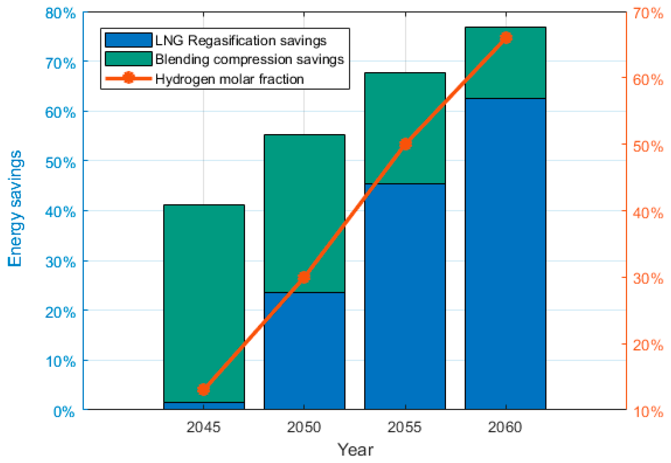
• The use of LOHC methodology collaterally implies the availability of a significant amount of energy in form of heat (around 1 MW per 870–1200 kg/h of naphthalene-decalin processed as stated in Table 10, depending on the mass flow of processed hydrogen) that can be easily used to perform energy saving measures by integrating these processes with LNG regasification. Within this paradigm, the designed system using a Rankyne’s cycle can supply more than 77% of the most energy-demanding process of traditional regasification when the produced natural gas is mixed with hydrogen (blending), which have been identified as the high-pressure compression (which takes 98% of the total energy consumption of the natural gas regasification process), being able to additionally reduce the seawater-related energy consumption on the heat exchange stages up to 62%.

References

1. Berstad, D.O.; Stang, J.H.; Nekså, P. Comparison Criteria for Large-Scale Hydrogen Liquefaction Processes. Int. J. Hydrogen Energy 2009, 34, 1560–1568. [Google Scholar] [CrossRef]
2. Cardella, U.; Decker, L.; Sundberg, J.; Klein, H. Process Optimization for Large-Scale Hydrogen Liquefaction. Int. J. Hydrogen Energy 2017, 42, 12339–12354. [Google Scholar] [CrossRef]
3. Baker, C.R.; Shaner, R.L. A Study of the Efficiency of Hydrogen Liquefaction. Int. J. Hydrogen Energy 1978, 3, 321–334. [Google Scholar] [CrossRef]
4. Nandi, T.K.; Sarangi, S. Performance and Optimization of Hydrogen Liquefaction Cycles. Int. J. Hydrogen Energy 1993, 18, 131–139. [Google Scholar] [CrossRef]
5. Faramarzi, S.; Nainiyan, S.M.M.; Mafi, M.; Ghasemiasl, R. A Novel Hydrogen Liquefaction Process Based on LNG Cold Energy and Mixed Refrigerant Cycle. Int. J. Refrig. 2021, 131, 263–274. [Google Scholar] [CrossRef]
6. Santos, L.F.; Costa, C.B.B.; Caballero, J.A.; Ravagnani, M.A.S.S. Kriging-Assisted Constrained Optimization of Single-Mixed Refrigerant Natural Gas Liquefaction Process. Chem. Eng. Sci. 2021, 241, 116699. [Google Scholar] [CrossRef]
7. Obayashi, Y.; Donovan, K. Kawasaki Heavy Says Liquefied Hydrogen Carrier Departs Japan for Australia. Reuters 2021. Available online: https://www.reuters.com/world/asia-pacific/kawasaki-heavy-says-liquefied-hydrogen-carrier-departs-japan-australia-2021-12-24/ (accessed on 17 November 2022).
8. Rafiq, M.Y.; Bugmann, G.; Easterbrook, D.J. Neural Network Design for Engineering Applications. Comput. Struct. 2001, 79, 1541–1552. [Google Scholar] [CrossRef]
9. Statistics Institute of the Canary Islands (ISTAC) Official. Population Figures by Sex, Provinces by Autonomous Communities and Years. Available online: https://www3.gobiernodecanarias.org/istac/statistical-visualizer/visualizer/data.html?resourceType=dataset&agencyId=ISTAC&resourceId=E30245A_000001&version=1.1#visualization/table (accessed on 8 October 2022).
10. Kalogirou, S.A. Artificial Neural Networks in Renewable Energy Systems Applications: A Review. Renew. Sustain. Energy Rev. 2001, 5, 373–401. [Google Scholar] [CrossRef]
11. Geng, Z.; Zhang, Y.; Li, C.; Han, Y.; Cui, Y.; Yu, B. Energy Optimization and Prediction Modeling of Petrochemical Industries: An Improved Convolutional Neural Network Based on Cross-Feature. Energy 2020, 194, 116851. [Google Scholar] [CrossRef]
12. del Real, A.J.; Dorado, F.; Durán, J. Energy Demand Forecasting Using Deep Learning: Applications for the French Grid. Energies 2020, 13, 2242. [Google Scholar] [CrossRef]
13. Hoang, H.M.; Akerma, M.; Mellouli, N.; Le Montagner, A.; Leducq, D.; Delahaye, A. Development of Deep Learning Artificial Neural Networks Models to Predict Temperature and Power Demand Variation for Demand Response Application in Cold Storage. Int. J. Refrig. 2021, 131, 857–873. [Google Scholar] [CrossRef]
14. Mir, A.A.; Alghassab, M.; Ullah, K.; Khan, Z.A.; Lu, Y.; Imran, M. A Review of Electricity Demand Forecasting in Low and Middle Income Countries: The Demand Determinants and Horizons. Sustainability 2020, 12, 5931. [Google Scholar] [CrossRef]
15. Lawrence, S.; Lee Giles, C. Conjugate Gradient and Backpropagation. In Proceedings of the International Joint Conference on Neural Networks, IEEE Computer Society, Como, Italy, 24–27 July 2000; pp. 114–119. [Google Scholar]
16. Red Eléctrica de España ESIOS REData API. Available online: https://www.esios.ree.es/es/balance?date=08-10-2022&program=P48&agg=hour (accessed on 8 October 2022).
17. Spanish State Meteorological Agency AEMET OpenData API. Available online: https://opendata.aemet.es/centrodedescargas/productosAEMET (accessed on 8 October 2022).
18. Tukey, J.W. Comparing Individual Means in the Analysis of Variance. Biometrics 1949, 5, 99–114. [Google Scholar] [CrossRef] [PubMed]
19. Tukey, J.W. Exploratory Data Analysis, 17th ed.; Addison-Wesley Publishing, Co., Ltd.: Reading, MA, USA, 1977. [Google Scholar]
20. Schafer, R.W. What Is a Savitzky-Golay Filter? IEEE Signal Process. Mag. 2011, 28, 111–117. [Google Scholar] [CrossRef]
21. Savitzky, A.; Golay, M.J.E. Smoothing and Differentiation of Data by Simplified Least Squares Procedures. Anal. Chem. 1964, 36, 1627–1639. [Google Scholar] [CrossRef]
22. Makrides, G.; Venizelou, V.; Kyprianou, A.; Theocharides, S.; Kaimakis, P.; Georghiou, G.E. Pv Production Forecasting Model Based On Artificial Neural Networks (Ann). In Proceedings of the 33rd European Photovoltaic Solar Energy Conference and Exhibition, Amsterdam, The Netherlands, 25–29 September 2017. [Google Scholar]
23. Consejería de Transición Ecológica de Canarias. Anuario Energético de Canarias; Gobierno de Canarias: Las Palmas de Gran Canaria, Spain, 2019.
24. Instituto Tecnológico de Canarias. Canary Islands Energy Transition Plan (PTECan); Gobierno de Canarias: Las Palmas de Gran Canaria, Spain, 2022.
25. Statistics Institute of the Canary Islands (ISTAC). Gasoline, Diesel and Fuel Oil Consumption by Periods and Provinces of the Canary Islands. Available online: http://www.gobiernodecanarias.org/istac/jaxi-istac/tabla.do?uripx=urn:uuid:8a6adeaa-03f8-49b1-9aab-e0ef1ce3de50&uripub=urn:uuid:0821d382-d388-4f45-9b07-7583f11a3250 (accessed on 9 October 2022).
26. Mokhatab, S.; Valappil, V.J.; Mak, Y.J.; Wood, A.D. Chapter 1—LNG Fundamentals. In Handbook of Liquefied Natural Gas; Mokhatab, S., Mak, J.Y., Valappil, J.V., Wood, D.A., Eds.; Gulf Professional Publishing: Boston, MA, USA, 2014; pp. 1–106. ISBN 978-0-12-404585-9. [Google Scholar]
27. Ramón, J.; Teresa, M.; Gotzon, A.; Guilera, G.J.; Tarancón, A.; Torrell, M. Hidrógeno: Vector Energético de Una Economía Descarbonizada; Fundación Naturgy: Madrid, Spain, 2020. [Google Scholar]
28. Lizarazo Suárez, R.; Cañas Rojas, D.G. Diseño Conceptual de Un Vaporizador de Gas Natural Licuado de Una Planta de Regasificación En Colombia. MetFlu 2015, 15, 17–23. [Google Scholar]
29. Khan, M.S.; Effendy, S.; Karimi, I.A.; Wazwaz, A. Improving Design and Operation at LNG Regasification Terminals through a Corrected Storage Tank Model. Appl. Therm. Eng. 2019, 149, 344–353. [Google Scholar] [CrossRef]
30. International Energy Agency (IEA). Spain Natural Gas Security Policy. Nat. Gas Secur. Policy 2022. Available online: https://www.iea.org/articles/spain-natural-gas-security-policy (accessed on 17 November 2022).
31. Seo, J.-W.; Yoo, S.-Y.; Lee, J.-C.; Kim, Y.-H.; Lee, S.-S. Process Simulation of the BOG Re-Liquefaction System for a Floating LNG Power Plant Using Commercial Process Simulation Program. J. Korean Soc. Mar. Environ. Saf. 2020, 26, 732–741. [Google Scholar] [CrossRef]
32. Environment Ministry of Spain. Manual Para La Gestión de Vertidos; Ministerio de Medio Ambiente: Madrid, Spain, 2007; pp. 234–235.
33. Fasihizadeh, M.; Sefti, M.V.; Torbati, H.M. Improving Gas Transmission Networks Operation Using Simulation Algorithms: Case Study of the National Iranian Gas Network. J. Nat. Gas Sci. Eng. 2014, 20, 319–327. [Google Scholar] [CrossRef]
34. Valderrama, J.O.; Silva, A. Modified Soave-Redlich-Kwong Equations of State Applied to Mixtures Containing Supercritical Carbon Dioxide. Korean J. Chem. Eng. 2003, 20, 709–715. [Google Scholar] [CrossRef]
35. Najjar, Y.S.H.; Mansour, A.R. Evaluation of Srk Equation of State in Calculating the Thermophysical Properties of Gas Turbine Combustion Gases. Int. J. Energy Res. 1987, 11, 459–477. [Google Scholar] [CrossRef]
36. Justo-García, D.; García-Sánchez, F.; Diaz Ramirez, N.L.; Díaz-Herrera, E. Modeling of Three-Phase Vapor–Liquid–Liquid Equilibria for a Natural-Gas System Rich in Nitrogen with the SRK and PC-SAFT EoS. Fluid Phase Equilib. 2010, 298, 92–96. [Google Scholar] [CrossRef]
37. Rao, P.C.; Yoon, M. Potential Liquid-Organic Hydrogen Carrier (Lohc) Systems: A Review on Recent Progress. Energies 2020, 13, 6040. [Google Scholar] [CrossRef]
38. Chen, X.; Gierlich, C.H.; Schötz, S.; Blaumeiser, D.; Bauer, T.; Libuda, J.; Palkovits, R. Hydrogen Production Based on Liquid Organic Hydrogen Carriers through Sulfur Doped Platinum Catalysts Supported on TiO2. ACS Sustain. Chem. Eng. 2021, 9, 6561–6573. [Google Scholar] [CrossRef]
39. Liu, X.; Michal, G.; Godbole, A.; Lu, C. Decompression Modelling of Natural Gas-Hydrogen Mixtures Using the Peng-Robinson Equation of State. Int. J. Hydrogen Energy 2021, 46, 15793–15806. [Google Scholar] [CrossRef]
40. Qian, J.W.; Jaubert, J.N.; Privat, R. Phase Equilibria in Hydrogen-Containing Binary Systems Modeled with the Peng-Robinson Equation of State and Temperature-Dependent Binary Interaction Parameters Calculated through a Group-Contribution Method. J. Supercrit. Fluids 2013, 75, 58–71. [Google Scholar] [CrossRef]
41. Aseeri, A.; Bagajewicz, M.J. New Measures and Procedures to Manage Financial Risk with Applications to the Planning of Gas Commercialization in Asia. Comput. Chem. Eng. 2004, 28, 2791–2821. [Google Scholar] [CrossRef]
42. Rehman, A.; Abdul Qyyum, M.; Ahmad, A.; Nawaz, S.; Lee, M.; Wang, L. Performance Enhancement of Nitrogen Dual Expander and Single Mixed Refrigerant LNG Processes Using Jaya Optimization Approach. Energies 2020, 13, 3278. [Google Scholar] [CrossRef]
43. López-Aguilar, K.; Benavides-Mendoza, A.; González-Morales, S.; Juárez-Maldonado, A.; Chiñas-Sánchez, P.; Morelos-Moreno, A. Artificial Neural Network Modeling of Greenhouse Tomato Yield and Aerial Dry Matter. Agriculture 2020, 10, 97. [Google Scholar] [CrossRef] [Green Version]
44. Government of Spain. Ley 12/1994 de Los Espacios Naturales de Canarias; Gobierno de Canarias: Las Palmas de Gran Canaria, Spain, 1994.
45. Canary Islands Government. Canary Island’s Industrial Development Strategy for the 2022–2027 Period; Gobierno de Canarias: Las Palmas de Gran Canaria, Spain, 2021.
46. Spain Port Authority. Management Report of the State-Owned Port System; Ministerio de Transporte, Movilidad y Agenda Urbana: Madrid, Spain, 2021.
47. Luque, A.; Martín Esquivel, J.; Dorta Antequera, P.; Mayer, P. Temperature Trends on Gran Canaria (Canary Islands). An Example of Global Warming over the Subtropical Northeastern Atlantic. Atmos. Clim. Sci. 2014, 4, 20–28. [Google Scholar] [CrossRef] [Green Version]
48. Mesko, J.; Ramsey, J. The Use of Liquefied Natural Gas For Peaking Service; INGAA Foundation, Inc.: Washington, DC, USA, 1996. [Google Scholar]
49. Strantzali, E.; Aravossis, K.; Livanos, G.A.; Chrysanthopoulos, N. A Novel Multicriteria Evaluation of Small-Scale LNG Supply Alternatives: The Case of Greece. Energies 2018, 11, 903. [Google Scholar] [CrossRef]
50. Xue, Q.; Wu, M.; Zeng, X.C.; Jena, P. Co-Mixing Hydrogen and Methane May Double the Energy Storage Capacity. J. Mater. Chem. A Mater. 2018, 6, 8916–8922. [Google Scholar] [CrossRef]
51. Wang, X.-J.; Liu, X.-Y. Liquefied Natural Gas Plant Heat Exchanger Fouling and Corrosion Analysis. Petro-Chem. Equip. 2015, 44, 68–71. [Google Scholar] [CrossRef]
Figure 1. LNG regasification—conventional process.
Energies 15 08682 g001
Figure 2. Block diagram of the methodology and calculations.
Energies 15 08682 g002
Figure 3. Proposed neural network architecture.
Energies 15 08682 g003
Figure 4. Simulated PFD for LNG regasification conventional process.
Energies 15 08682 g004
Figure 5. LOHC hydrogenation-dehydrogenation generic process.
Energies 15 08682 g005
Figure 6. Simulated PFD for LOHC hydrogenation-dehydrogenation processes.
Energies 15 08682 g006
Figure 7. Simulated PFD for the hydrogen-NG blending compression stage.
Energies 15 08682 g007
Figure 8. Simulated PFD for the energy integration system.
Energies 15 08682 g008
Figure 9. Tukey test results.
Energies 15 08682 g009
Figure 10. Filtering process results.
Energies 15 08682 g010
Figure 11. Neural network training results: (a) temperature module; (b) power demand module. Note how because of the use of the Bayesian Regularization algorithm for the power demand module, no correlation between validation samples and neural network results are presented, as full correlation (R = 1) is forced by the algorithm itself only for that category of samples.
Energies 15 08682 g011
Figure 12. Power demand historical data error: (a) relative error; (b) absolute error histogram grouped by sample type (note that x axis values are in MWhe).
Energies 15 08682 g012
Figure 13. Neural network prediction results.
Energies 15 08682 g013
Figure 14. LOHC reactor conditions optimization results: the hydrogenation process (left) and the dehydrogenation process (right).
Energies 15 08682 g014
Figure 15. Energy savings and hydrogen mole fraction in blending mixture.
Energies 15 08682 g015