1. Introduction
Cyberattacks are continuously increasing, as highlighted by several sources. The COVID-19 pandemic over the last three years accelerated an existing trend, as highlighted in the survey by
Georgescu (
2021). The number of companies experiencing more cybersecurity incidents is up to 60%. In particular, a 13% increase in ransomware was observed
Verizon Risk Team (
2022). Moreover, a threefold increase in Remote Desktop Protocol (RDP) attacks occurred
Georgescu (
2021). Though the shift to remote work during the pandemic may be considered the trigger for many of the latest trends, the rising trend of cybersecurity incidents has been going on for several years. After analyzing data provided by Advisen, a US-based organization that acquires and sells cyberloss and incident data to insurers, it was found that reinsurers, brokers, and cybermodeling firms,
Palsson et al. (
2020) experienced a steady increase in cyberincidents over the years, covering since 2018.
Xu et al. (
2018) tried to find a model for the time series of hacking breaches, observing a sharp decrease in the interarrival time of incidents (hence, an increase in their frequency) starting in 2016. Going a bit backwards,
Wheatley et al. (
2016) highlighted that the overall frequency of large data breaches has increased in the period ending in 2015 (due especially to outside-the-US events), driving the growth in the overall volume of breached records. Finally,
Maillart and Sornette (
2010) identified faster-than-exponential growth from 2000 to 2006, i.e., roughly twenty years ago. That marks a very long period of practically uninterrupted growth of cybersecurity issues. It has to also be noted that not all cyberincidents are reported:
Sangari and Dallal (
2022) have proposed an approach to estimate unaccounted incidents and correct the count of incidents.
Bothos et al. (
2021) adopt an econometric model to predict the probability of an attack, considering bug bounties and the prizes offered for white-hat hackers in a time series model. A contagion model for the attack is instead suggested by
Chiaradonna and Lanchier (
2021), where contagion spreads through the edge of the network, moving with different probabilities towards lower-level and higher-level assets. Contagion is similarly analyzed by
Xu and Hua (
2019), where both Markovian and non-Markovian models are employed. Machine learning is instead employed to predict attacks in (
Yeboah-Ofori et al. 2021).
Aside from the technical disruption caused by cyberattacks, their economic consequences have been a significant issue of concern in cybersecurity management since long ago, as reported in the economic-grounded cyber-risk management framework put forward by
Jerman-Blažič et al. (
2008);
Rodrigues et al. (
2019). Costs related to cybercrime belong to several categories, as listed by
Eling and Wirfs (
2019). The measurement (or estimation) of the losses caused by cyberattacks has been addressed by several authors. The use of Value-at-Risk as a metric for cyberlosses has been advocated by
Erola et al. (
2022). A similar approach addressing extreme risks is considered by
Strupczewski et al. (
2018), who exploit the SAS OpRisk Global Database. Additional metrics, such as the risk-adjusted return on security investment and risk-adjusted return on capital, have been proposed by
Orlando (
2021).
Giudici and Raffinetti (
2022) proposed the use of ordinal regression and Shapley values instead to describe the level of cyber-risk as a means to progress towards explainability. In addition to the immediate consequences of attacks, being exposed to cyberattacks has far-reaching consequences on the market value of companies, as investigated by
Arcuri et al. (
2017) and
Hovav and D’Arcy (
2003).
Lin et al. (
2021) have reversed this point of view, using the public stock market response to estimate cyberlosses. A similar reverse approach has been put forward by
Woods et al. (
2021), who use particle swarm optimization to derive a cyberloss distribution from cyberinsurance prices. The estimation of the actual costs is a research theme itself, as shown in several papers, e.g., by
Hua and Bapna (
2013);
Kamiya et al. (
2020);
Poufinas et al. (
2018);
World Economic Forum (
2015) and
The Ponemon Institute (
2016). An econometric approach relating cyberlosses to company size has been proposed by
Yamada et al. (
2019). The availability of data, especially through open access databases, has been highlighted as a further problem that hampers all attempts to tackle cyber-risk and devise a proper cyber-risk management strategy
Cremer et al. (
2022).
From an economic point of view, strategies to manage cyber-risks have the natural aim of minimizing the overall loss, where the term
overall implies that we must factor in the economic values of many terms in the budget equation. Under this aspect, the set of strategies that we may consider in cyber-risk management is not at all different from the taxonomy of strategies available for general risk management
Scala et al. (
2019), i.e., the three categories of risk avoidance, risk transfer, and risk mitigation (or a combination thereof), as described by
Paté-Cornell et al. (
2018) and
Refsdal et al. (
2015). A historical survey of cyber-risk management with an eye on the future is reported by
McShane et al. (
2021).
While risk avoidance is not a viable option in many cases, since it would imply a significant sacrifice of usability, as shown by
Murphy and Murphy (
2013), we can focus on the latter two.
Risk transfer is typically carried out by buying an insurance policy, where risk is transferred from the insured to the insurer upon paying a premium. Several efforts have been devoted to premium computation formulas. An approach based on the first two statistical moments of loss (mean–variance) has been employed by
Mukhopadhyay et al. (
2019), while an approach based on a more accurate (and demanding) statistical characterization of losses (up to the fourth moment) has been proposed by
Naldi and Mazzoccoli (
2018) and
Mazzoccoli and Naldi (
2020a). Instead,
Young et al. (
2016) have proposed incorporating a discount in premium formulas and incentivizing all actions aimed at reducing the loss. That proposal has been advocated by
Rosson et al. (
2019) in the context of the power sector. While these approaches assume loss to be known (or at least estimated),
Antonio et al. (
2021) have proposed to incorporate the network structure into pricing to account for the presence of clusters in the diffusion of attacks.
Lopez and Thomas (
2022) have analyzed the possible use of parametric insurance, where a parameter related to the loss is employed instead of the true loss to determine compensation; the parametric approach allows setting up insurance policies when the amount of information about risk is limited. Moreover, the adoption of security audits to design insurance contracts more accurately has been put forward by
Khalili et al. (
2018). Additionally, the relationship between insurance and pricing sustainability has been investigated by
Mastroeni et al. (
2019). The traditional distinction between insured and insurer is abandoned in (
Vakilinia and Sengupta 2018), where a coalitional approach is proposed, with organizations playing the role of insured and insurer at the same time, adopting crowdfunding, or outsourcing a common insurance platform. An excellent survey of cyberinsurance has been carried out by
Marotta et al. (
2017).
Risk mitigation is instead carried out by investing in tools and procedures that can help to reduce the probability of success for cyberattacks and/or the extent of losses when cyberattacks succeed.
Mayadunne and Park (
2016) have related those investment decisions to the risk-taking attitude of the company.
Naldi et al. (
2018) have investigated the liability consequence of not investing enough in security. The optimization of investment has been the subject of many papers, which mainly differ on the relationship between investment and security performance. The seminal paper for such an approach is due to
Gordon and Loeb (
2002). A mixed-integer linear programming formulation has been adopted in the context of Industry 4.0 supply chains by
Sawik (
2020). Instead, most papers adopt a straightforward net profit maximization.
Wu et al. (
2015) employ a game-theoretic approach to analyze the investment strategies of two interconnected firms under different types of attack (targeted vs opportunistic). The optimal trade-off between investing in knowledge and expertise versus investing in deploying mitigation measures has been investigated by
Wang (
2019). The spread of attacks is described through a Susceptible–Infected–Susceptible (SIS) model in
Mai et al. (
2021), where security investment, recovery costs, and economic losses are considered.
The mixed approach, consisting in investing in reducing the vulnerability and buying an insurance policy to cover the residual risk, was first dealt with by
Young et al. (
2016), and has been further explored by
Mazzoccoli and Naldi (
2020b), who have examined the robustness of risk management strategic choices when the information about the system under attack is uncertain.
Skeoch (
2022) has also embraced a similar approach, but employing a utility function (either logarithmic or exponential) and adopting a percentage premium. The analysis has then been extended by
Mazzoccoli and Naldi (
2021) to the case of a firm with multiple branches and interdependencies, chasing the problem introduced by
Xu et al. (
2019). The importance of interdependencies is also examined by
Uuganbayar et al. (
2021), who examine the possible incentivizing impact that cyberinsurance has on security investments in the case of interdependence. While these studies are concerned either with the variety of attacks or the variety of targets, a slightly different subject is analyzed by
Yaakov et al. (
2019), who consider choosing among a variety of countermeasures, i.e., including specific mitigation tools (such as intrusion detection systems and firewall) and reporting the results of a game played by fictional decision makers.
When pursuing a mitigation approach (or a mixed one), a crucial role is played by the so-called security breach function, i.e., the function describing the impact of investments on the probability that the attack is successful. Since that function returns a probability value, modeling the vulnerability through the security breach probability function allows us to fulfill the risk description step, which is the third step involved in any risk analysis process, as set in
Aven (
2011). Moreover, it allows us to evaluate the risk through the computation of the expected value of losses when we associate a loss with each breach event. The choice of a suitable model for the security breach probability function is then a fundamental step in a probabilistic risk assessment (PRA) approach to risk analysis. Though several functions have been proposed for that task, we cannot list a single attempt to line them up and examine them using the same systematic approach. The correct choice of the function, often tailored to the specific type of attack, is essential to properly choose the amount to invest in security. In this paper, we propose a description and analysis of all the breach probability functions that appeared in the literature by adopting a unifying approach. In particular, we provide the following contributions:
It is to be noted that we strongly advocate the principle that there is no one size fits all. The range of investment choices may be very large, since they may differ not just for their size (monetary value) but also by the device (e.g., investing in antivirus software rather than in a network firewall), the technology employed (e.g., adopting a software based on known malware signatures rather than on a machine learning approach), or the system location where the security devices are placed (e.g., on any single machine or through a centralized approach). Moreover, the impact of each investment choice depends on the type of attack, so some choices are better suited to defend against a specific type of attack.
2. Security Breach Probability Models
The security breach probability function describes how the vulnerability of the system (here embodied by the probability of a breach) is reduced when the company invests in security, i.e., the relationship between investments and security levels. Though several models have been proposed for that function, there are some common features that those models share, i.e., some fundamental properties. In this section, we first outline those properties that any security breach probability function should possess and then provide a detailed survey of the models proposed in the literature.
2.1. Definitions
Before dealing with the properties of the security breach function, we define what it describes more precisely. We adopt the glossary provided by the Society for Risk Analysis
Aven et al. (
2018), but we provide a bridge with the terms employed in the cybersecurity literature where the standards in the two communities differ.
The event of interest here (see the Definition 1.7 of
Aven et al. (
2018)) is a data breach, i.e.,
1 “an incident where information is stolen or taken from a system without the knowledge or authorization of the system’s owner.” This definition is consistent with what the authors of the three papers providing the model described here state. Namely, Gordon and Loeb define the security breach probability function as the function providing the probability that an information set is breached
Gordon and Loeb (
2002). Hausken and Wang follow suit, providing alternative models for exactly the same event
Hausken (
2006);
Wang (
2017). For all purposes, the information set breach they consider can be considered a synonym of a data breach.
We do not deal here with the adverse consequences of that breach. The severity of the damage could be quantified (as Gordon and Loeb do) by the amount of money that is lost as a consequence of the breach (see Definition 1.8 of
Aven et al. (
2018)). As an example of studies considering the influence on consequences other than vulnerability,
Wang (
2019) analyze separately the role of investments in separately reducing threats (i.e., the probability of an attack), vulnerability (i.e., the probability that an attack succeeds), and impact (i.e., the loss if an attack succeeds).
The threat here is represented by the intention of the attacker (who wishes to get hold of the data) to initiate an attack (see the Definition 1.18 of
Aven et al. (
2018)).
The vulnerability in the risk analysis context (as reported in the Definition 1.19 of
Aven et al. (
2018)), i.e., conditional on the risk event, is the probability that a data breach occurs. In the cybersecurity economics literature
Gordon and Loeb (
2002);
Hausken (
2006);
Wang (
2017), a distinction is made between the vulnerability when an investment in security is made (which is the breach probability function for which we later provide the relevant models) and the vulnerability when no investments are made (which is simply called vulnerability in the cybersecurity economics literature). For the sake of maintaining the distinction while employing the SRA terminology, we refer to the breach probability function as simply the vulnerability, and use the term
a priori vulnerability to denote the vulnerability in the absence of investments.
The vulnerability is expected to be lower than the a priori one, as investments are made in cybersecurity. If we indicate the investment by , and the a priori vulnerability as , the resulting vulnerability is , also known as as security breach probability function. Its notation explicitly shows that it is a function of both the a priori vulnerability and the investment. Both the a priori vulnerability and the vulnerability are measured as probabilities. Its range is then defined as .
The way we act on the risk here is just through mitigation (see Definition 3.5 of the SRA glossary
Aven et al. (
2018)). Risk is not canceled but just reduced. No risk avoidance or risk transfer measures are contemplated here. We can envisage several mechanisms to reduce risks. Money can be spent on any of the countermeasures typically adopted to prevent breaches from occurring. For example, data breaches may be reduced by:
Purchasing antivirus software;
Installing firewalls inside the network;
Deploying tighter access control policies;
Renewing and updating the ICT infrastructures;
Having employees attend training courses to increase their awareness of cybersecurity risks and develop more cautious behavior.
Coming back to the security breach probability function, it may be more convenient to deal with the normalized breach probability function, since we are mainly interested in how investments reduce the breach probability down from
v:
2.2. Fundamental Properties
We expect any security breach probability function to possess several essential characteristics. Here, we consider a superset of those established in
Gordon and Loeb (
2002), which we may include some alternatives. These properties are reported hereafter in full:
- :
, ;
- :
, ;
- :
,
- :
, and ;
- :
, and ;
- :
- :
, ;
- :
, and .
Property concerns the impact of the a priori vulnerability. If the information set is completely invulnerable, it will remain perfectly protected for any information security investment, including a zero investment.
Property concerns the behavior of the system if no investment in security is made. In that case, the vulnerability of the system equals its a priori vulnerability v.
Property states that the probability of a security breach can be made to be arbitrarily close to zero by investing sufficiently in security.
Property embodies the general requirement that information is made more secure as the company invests more in security.
Properties all concern the second derivative, i.e., the change in the decay of the breach probability as the company invests more in security. It is to be noted that these properties are alternative to each other.
Under Property , the vulnerability decreases at a slower rate as the investment grows. This property embodies the law of diminishing returns. If the breach probability follows this property, investing beyond a certain threshold does not pay because the reduction in the expected loss due to the cyberattack is not enough to justify the additional investment.
Property again concerns the rate at which the effectiveness of security investments changes. In this case, the breach probability decreases first at a slow rate (when investments are very low) but then gathers momentum and is significantly abated as the investment grows to end up approaching zero slowly when investments get even bigger.
Under Property , the negative slope of the security breach function becomes even more negative as investments grow. Coupling Property with , we obtain a concave breach probability function, where investments have larger effectiveness as they grow. Of course, a continuing concavity would bring the breach probability below zero, which would violate probability principles, so that this model is valid up to the value such that .
Finally, Property simply embodies the case of a linear breach probability function.
In the literature, we found nine functions that possess all these properties (i.e., Properties through and one of the alternatives):
Gordon–Loeb Class One;
Gordon–Loeb Class Two;
Hausken Class Three;
Hausken Class Four;
Hausken Class Five;
Hausken Class Six;
The Exponential Power Class;
The Proportional Hazard Class;
The Wang Transform Class.
In the following subsection, we describe each of them and analyze their properties. For each model, we roughly follow the same pattern: (a) introducing the mathematical function that describes the model; (b) checking that it possesses the five fundamental properties; (c) identifying the functional formal that relates the breach probability to the a priori vulnerability and investments; and (d) describing the role of parameters.
2.3. Gordon–Loeb Class One Model
The first security breach probability function we examine is the Gordon–Loeb Class One function (GL1 for short), introduced by
Gordon and Loeb (
2002). It has the following expression
where the parameters
and
measure of the productivity of information security.
This function possesses Properties and Property :
- :
;
- :
;
- :
;
- :
;
- :
.
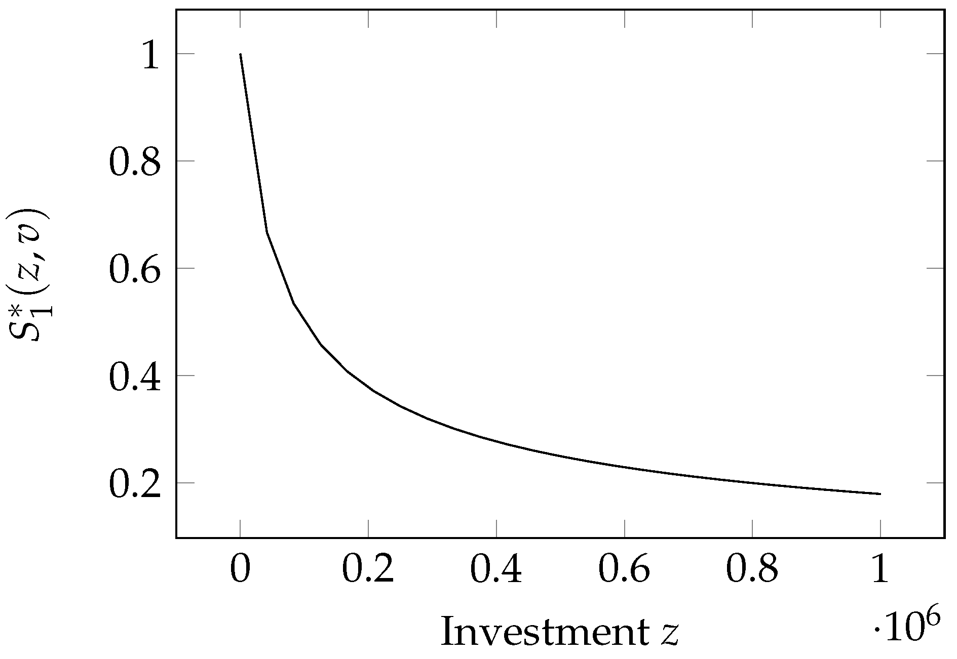
The model is graphed in
Figure 1. It depends linearly on the a priori vulnerability. The relationship with investments is a bit more complex since we have a modified (scaled and shifted) power-law functional form.
The two parameters
and
modulate the relationship with the investments. Values provided for them in the seminal paper by
Gordon and Loeb (
2002) are
and
. It is to be noted that, since
acts as a scaling factor for
z, its value also depends on the unit of measurement chosen for the investment (which is dollars in
Gordon and Loeb (
2002)).
A special form of the GL1 model (namely, when
) has been independently derived by
Huang and Behara (
2013) for the case of targeted attacks on a particular node (one-to-one attacks). The mathematical equivalence of the GL1 model and the model proposed by Huang and Behara has been proven by
Naldi et al. (
2018). In their paper,
Huang and Behara (
2013) employ the value
.
This model was used by
Mayadunne and Park (
2016) to analyze the information security investment through the simplified functional form of the security breach probability function used in
Huang and Behara (
2013). The GL1 model was also employed by
Hua and Bapna (
2013) to determine the sensitivity of the investment in security. Then, it was employed by
Gao et al. (
2015), who extended the GL1 model, combining the latter function with factors that took into account risk and investment correlation among multiples companies.
Gordon et al. (
2015) used this function to analyze the investment in security considering some target level of cybersecurity. In the same year,
Wu et al. (
2015) demonstrated, using this model, that the optimal security investment level of an interconnected firm against targeted attacks is different from that against opportunistic attacks and discussed two economic incentives to motivate firms, or rather liability and security information sharing. Recently, this model was used in a risk management framework by
Gordon et al. (
2020) to derive a cost-effective spending level on cybersecurity activities. A dynamic extension has also been proposed by
Krutilla et al. (
2021).
Mai et al. (
2021) employ a simplified version of this model, where
and
.
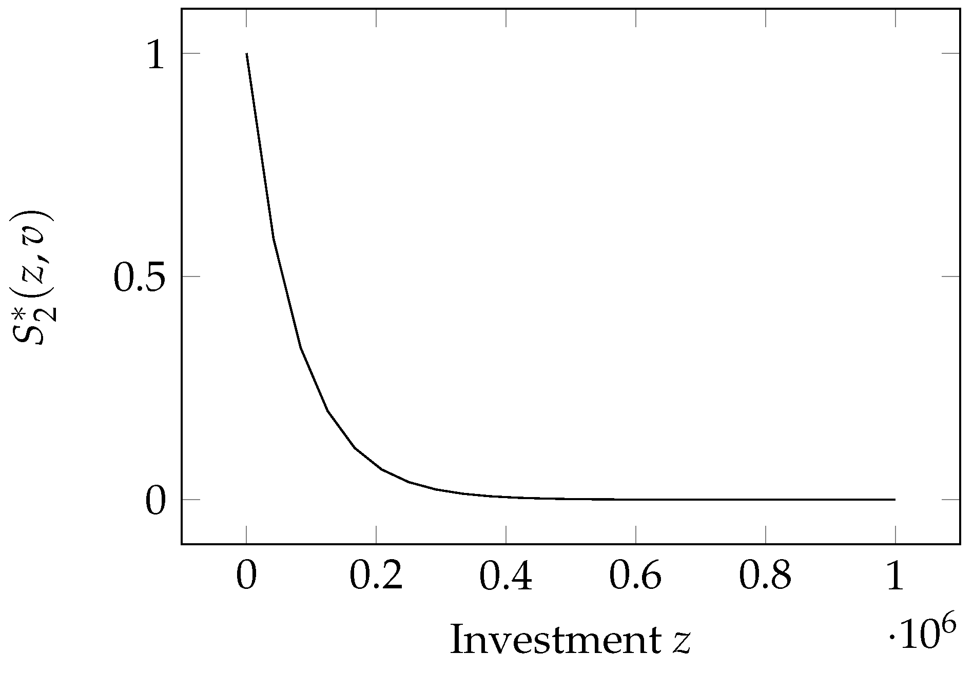
2.4. Gordon–Loeb Class Two Model
The second security breach probability function is again due to Gordon and Loeb. It was introduced along with the GL1 model in their seminal paper (
Gordon and Loeb (
2002)). Accordingly, we call it the Gordon–Loeb Type Two function (GL2 model for short). Its mathematical expression is
where
is a coefficient that measures the effectiveness of security investments: the larger
is, the more effective the investment. The coefficient
roughly plays the same role as
in the GL1 model, i.e., a scaling factor for the investment
z. It is, however, the only parameter in the function, while the GL1 model has two.
Unlike the GL1 model, the GL2 model bears a nonlinear relationship with both the investment, and the a priori vulnerability v.
As in the case of the GL1 model, the GL2 model possesses all the properties of and :
- :
;
- :
;
- :
;
- :
;
- :
.
Similarly to the GL1 model,
Huang and Behara (
2013) derived a model whose mathematical expression is identical to the GL2 model for attacks that propagate epidemically over a scale-free network (opportunistic attacks). Again, the equivalence of the GL2 model and that proposed by
Huang and Behara (
2013) was proven by
Naldi et al. (
2018).
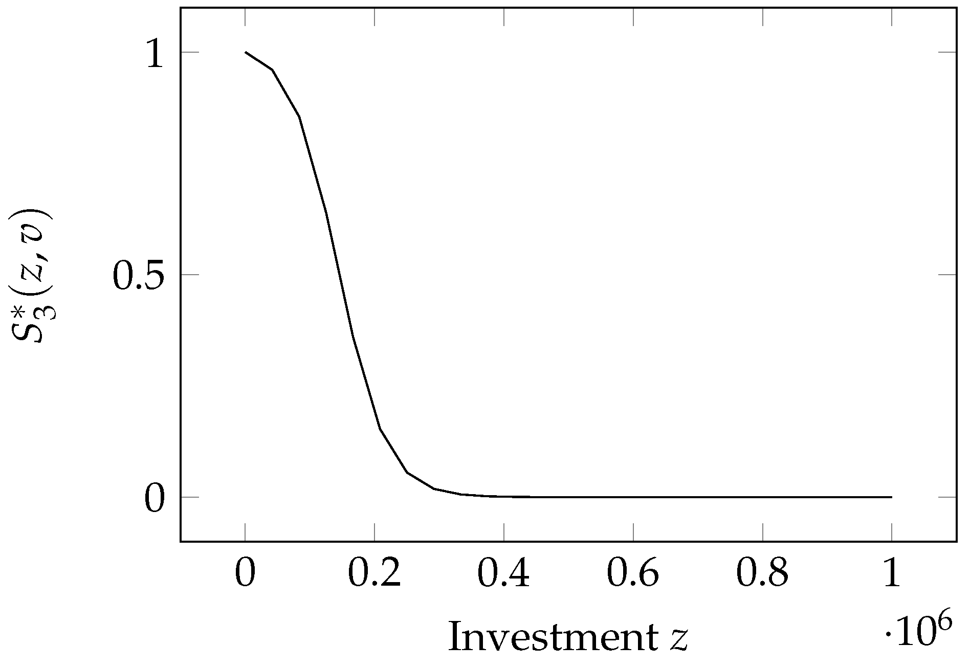
2.5. Hausken Class Three Model
Hausken (
2006) introduced an alternative breach probability function that replaces one assumption of both GL models, namely the law of diminishing returns embodied by Property
. That assumption is replaced by Property
, where small investments have a very small impact, but vulnerability is greatly lowered when investments reach a critical mass. If investments get even bigger, the law of diminishing returns applies again in full. The model proposed by Hausken, called by Hausken himself Class Three (hereafter H3 model for short) to follow the numbering initiated by Gordon and Loeb, is
where
and
are coefficients that measure the productivity of the information security. Again, the coefficient
is a scaling coefficient for the investment and plays then the same role as
in the GL1 model and
in the GL2 model. The resulting breach probability function follows a logistic decrease, as can be seen in
Figure 3.
This function satisfies Properties :
- :
;
- :
;
- :
;
- :
.
As hinted, it also possesses Property
in place of
. The intermediate investment
appearing in Property
can be found by zeroing the second derivative with respect to the investment
z of the security breach probability function:
This security breach probability function was used by
Hua and Bapna (
2013) to determine the sensitivity of the optimal investment in security to confront losses caused by cyberterrorists and hackers, similarly to what they did for the GL1 model.
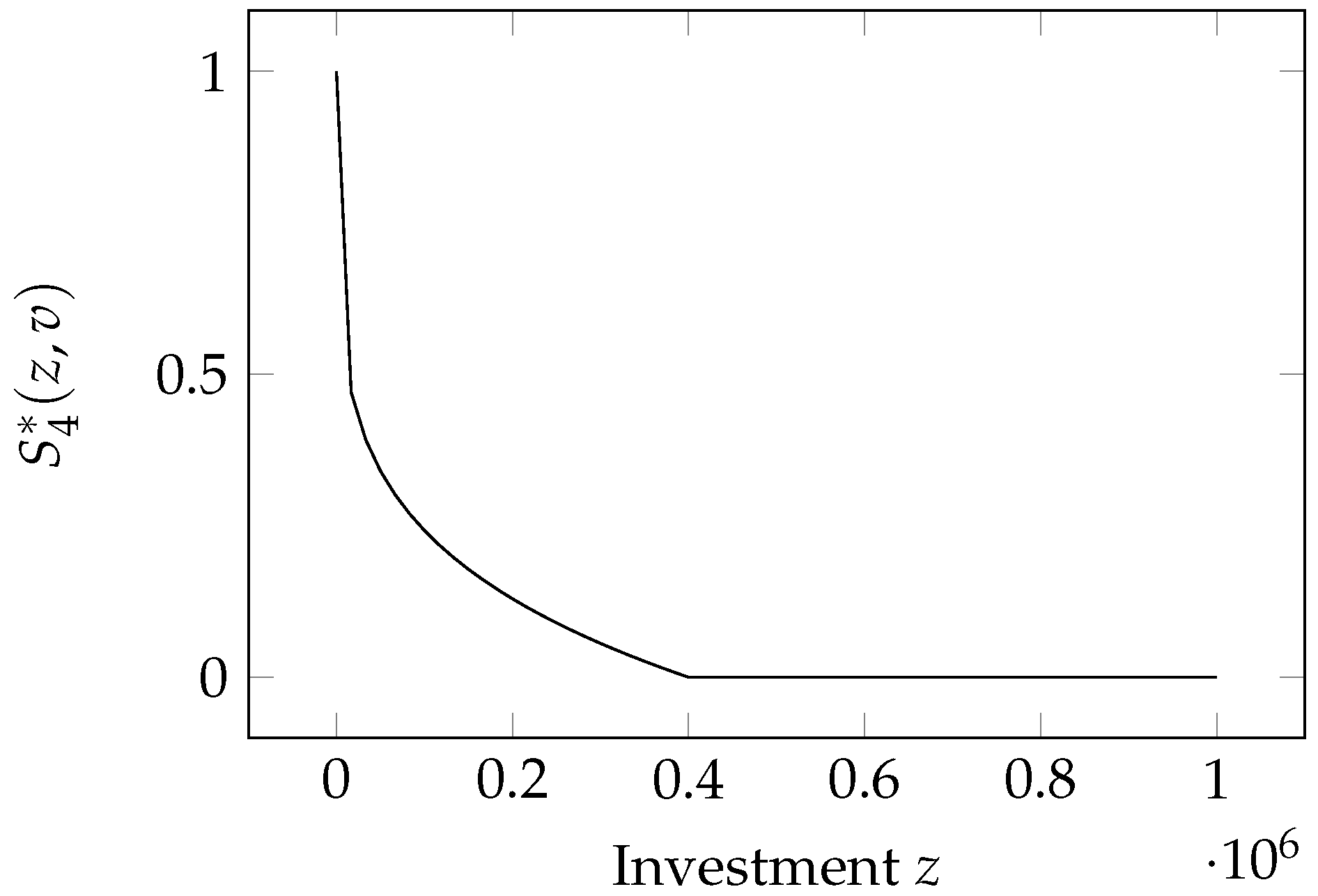
2.6. Hausken Class Four Model
This is again a model proposed by
Hausken (
2006) and is called Class Four, following the numbering initiated by Gordon and Loeb.
Its mathematical expression is
where
and
.
The model is graphed in
Figure 4. It combines some functional relationships seen in the previous models since it is linear in the a priori vulnerability but exhibits a shifted-and-scaled power-law dependence on the investment. A new feature is, however, the possibility of achieving total invulnerability (i.e., zero breach probability) if the investment is large enough (namely larger than
). Hausken himself admitted that such total invulnerability is quite unrealistic, which leads to two conclusions: (a) the threshold
must be set at very high values; (b) the interesting part of the model is that where
.
Keeping in mind condition (b), the properties stated in
Section 2.2 must be checked under the hypothesis that
. In that case, we see that the Hausken Class Four model possesses Properties
and, again,
, as the GL1 and GL2 models:
- :
;
- :
;
- :
;
- :
;
- :
.
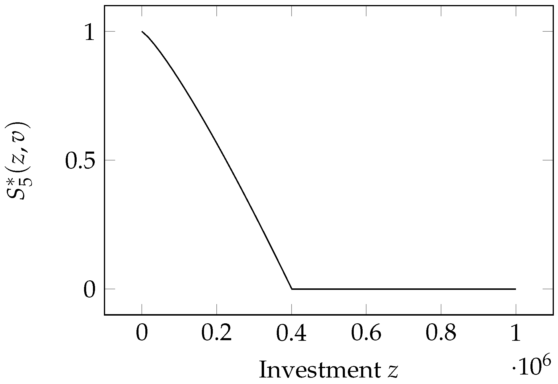
2.7. Hausken Class Five Model
Here, we again have a model proposed by
Hausken (
2006). The breach probability appears to have the same mathematical expression as the Hausken Class Four model:
The coefficient
plays the same role of scaling the contribution of the investment as
in GL1,
in GL2, and
in H3. In addition, it assumes again (as in the H4 model) that the system can be made invulnerable by investing enough in security. Namely, the threshold beyond which the breach probability is zero is
. However, the exponent
k now lies in the
range, which has an impact on the sign of the second derivative of the breach probability function.
This function possesses the properties plus :
: ;
: ;
: when ;
: ;
: .
Small investments are then relatively ineffective but become increasingly effective as they grow, till reaching the point of complete invulnerability when
, as can be seen in
Figure 5.
2.8. Hausken Class Six Model
Here, we have the last of the models proposed by
Hausken (
2006), which we call hereafter H6 for brevity. The breach probability is a linear function of the investment
This model can be seen as a special case of the H4 model, with the simple name change in the scaling coefficient
, and when we remove the limitation on the exponent
k and set it as
. The model is graphed in
Figure 6.
The H6 model keeps the same assumption as models H4 and H5 that total invulnerability can be achieved if investments are large enough, namely beyond the threshold . As in the previous cases, we are interested in examining the properties of this function when it still exhibits a degree of vulnerability, i.e., when .
It possesses the following properties:
: ;
: ;
: when ;
: ;
: .
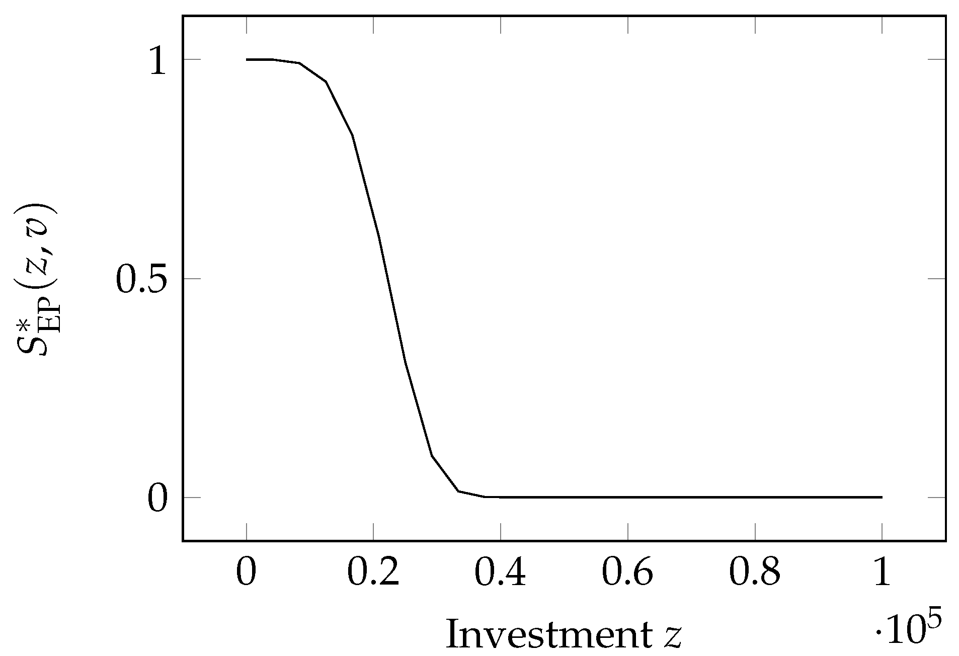
2.9. The Exponential Power Class Model
This model is one of the three proposed by
Wang (
2017). Its formulation is a bit different from the models examined so far, since Wang assumes that the system is totally vulnerable if there is no investment in security, i.e.,
. In addition, Wang considers a benchmark investment
B and defines the breach probability as a function of the normalized investment
. His breach probability function is then
where
.
We can safely remove the former assumption to make the model more general. Since removing the assumption that
is akin to removing the normalization concerning the a-priori vulnerability, the breach probability function
can be seen as the un-normalized version of the original function proposed by Wang:
where
.
Similarly to the Hausken Class Three model, the Exponential Power Class possesses Properties and
- :
;
- :
;
- :
since ;
- :
, again since ;
- :
.
As to Property
, we note that the term preceding the square bracket is always negative, since
, so that the second derivative is negative if
, i.e., if the investment is
We then have a breach probability function that is concave for low investments and convex (concave upward) for high investments; the marking point between low and high investments being given by Equation (
11). This inflection point marks the switch to a lower marginal impact of investments.
The Exponential Power Class function has been employed by
Feng et al. (
2020) to investigate the competition between two cloud providers trying to sell their cloud security services while optimizing their investments to maximize their profits.
Feng et al. (
2020) adopted
and
as example values for the model parameters.
Wang (
2019) derived an optimal mix of cybersecurity investments in
knowledge and expertise versus
deploying mitigation measures using this function.
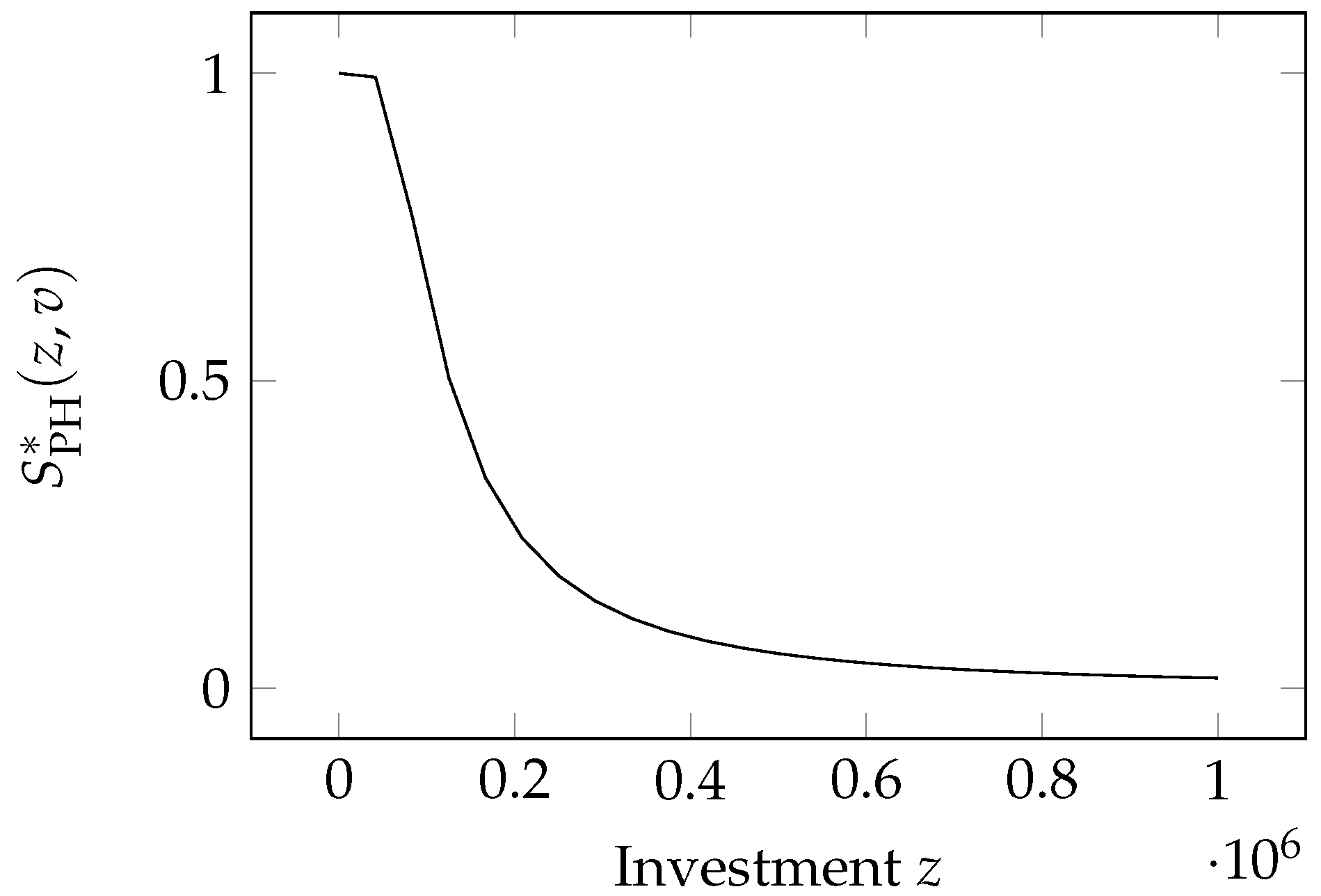
2.10. The Proportional Hazard Class Model
Wang (
2017) introduced a second model, which he called the Proportional Hazard class, again adopting normalized investment as the independent variable (with the same benchmark investment
B as a normalization parameter). Its form is
the parameter
is the same as that appearing in the Exponential Power Class and is invariant to changes in the benchmark investment
B. The model is graphed in
Figure 8.
Following the same transformation indicated in the first step of Equation (
10), we obtain the breach probability function exponential power class
where
.
The security breach probability function follows properties and , since the domain of this function is . The Property must be verified computing the limit in
;
since ;
, again since ;
;
The second derivative in Property
is negative if
, i.e., if the investment is:
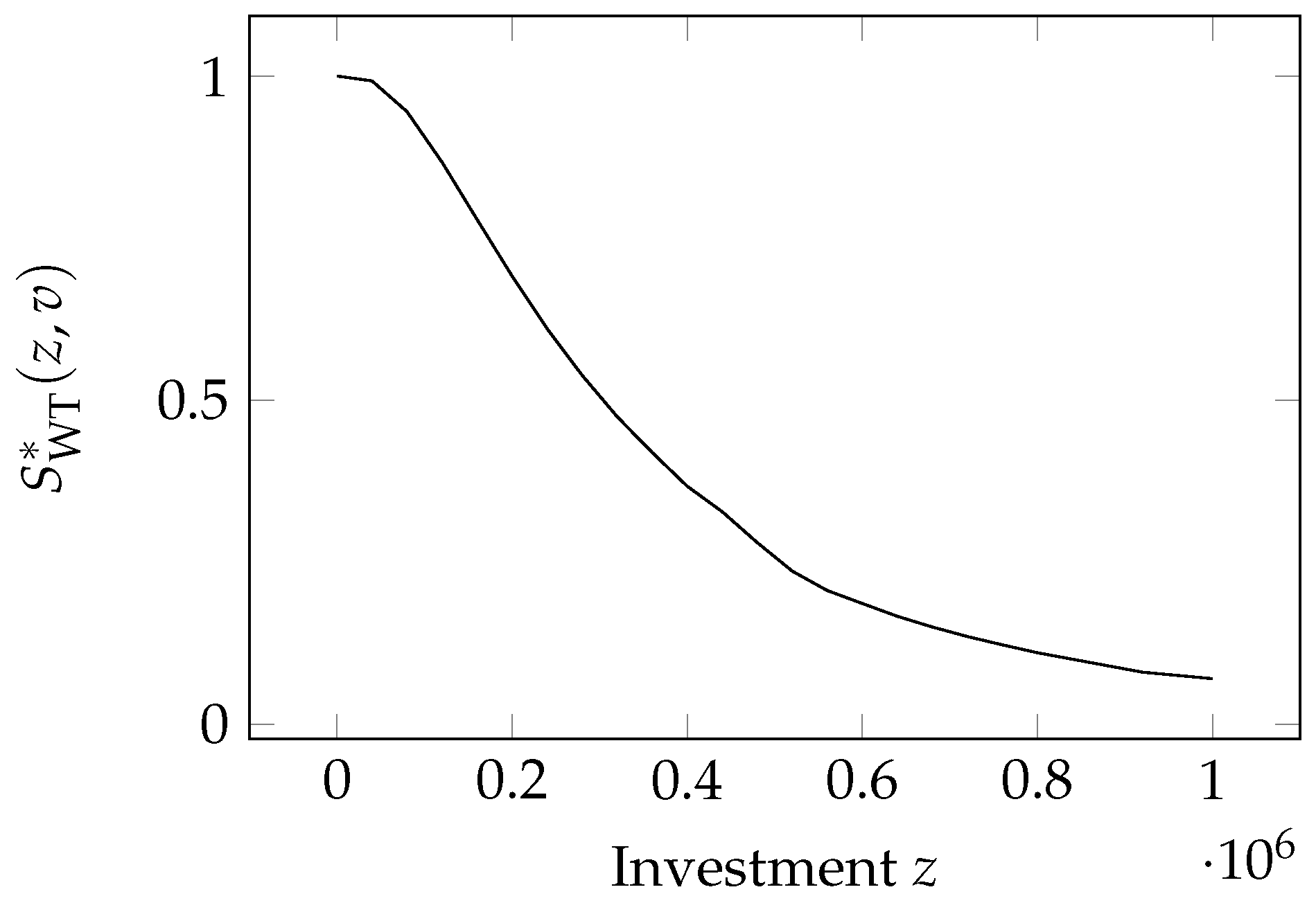
2.11. The Wang Transform Class
The last security breach probability function we analyze employs the Wang Transform. It was introduced by
Wang (
2017) and then used in the paper by
Feng et al. (
2020), WT, and has the form
where
,
is the cumulative distribution function for the standard normal distribution, and
has the same meaning as in the Exponential Power and the Proportional Hazard classes. The model is plotted in
Figure 9.
This function possesses the four fundamental properties and
;
;
;
;
Additionally, zeroing the second derivative with respect to the investment
z of the security probability breach function, the intermediate investment
z can be found
This model has been employed by
Feng et al. (
2020).
3. Sensitivity of the Security Breach Probability Functions
As summarized in
Table 1, all the security breach probability models reviewed in
Section 2 depend on either a single parameter or two parameters. Though those parameters do not change the functional relationship between the breach probability and the investments, their correct determination is essential for the accurate representation of reality. Some effort has been devoted to their correct calibration, e.g., by
Naldi and Flamini (
2017). Similarly, some effort should be spent on analyzing how their value influences the above relationship, i.e., the sensitivity of the breach probability to those parameters. Any calibration task is unavoidably marred by a degree of incertitude on the correct value of the parameters. Those parameters that bear a greater impact on the breach probability must be determined with greater accuracy. In this section, we analyze the sensitivity of the breach probability functions to their parameters in all the models examined. For that purpose, we employ the quasi-elasticity function. After defining that function, we evaluate it for all the models described in
Section 2.
In the following, we use the values reported in
Table 2 to plot the quasi-elasticity functions. Unless otherwise stated, we assume
and
.
3.1. Quasi-Elasticity
The notion of sensitivity in economics has typically been measured through elasticity, i.e., the measure of the percentage change in the response variable when an input variable changes by 1%. The description is well reported in textbooks, such as in Chapter 17 of
Arnold (
2008) or Chapter 6 of
Krugman and Wells (
2009). It has been widely employed in the context of cybersecurity risk to measure the sensitivity of the optimal investment with respect to the two parameters in the GL1 model in
Mazzoccoli and Naldi (
2020b).
However, here we are concerned with the sensitivity of the breach probability function, which intrinsically lies in the [0,1] range, so it is more appropriate to employ the quasi-elasticity instead, which measures the absolute change in the response variable when the input variable undergoes a relative change. Quasi-elasticity has been employed by
Naldi et al. (
2019) to measure the trade-off between fairness and profit in project selection.
In our case, we define the quasi-elasticity of the security breach probability function with respect to a generic parameter
x of the breach probability function:
By multiplying the quasi-elasticity by 100, we obtain the change in the security breach probability due to a
increase in the breach probability function parameter.
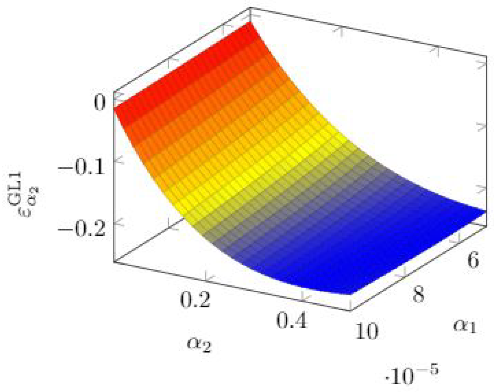
3.2. Gordon–Loeb Class One Model Elasticity
Since the Gordon and Loeb Type One model is governed by two parameters (
and
), we compute the quasi-elasticity function according to Equation (
17) for both.
The resulting quasi-elasticity for
takes the following form
From this formula, we already see that the quasi-elasticity is always negative: the breach probability decreases when
grows. However, the rate of change depends very much on the other parameter. In
Figure 10, we see that
plays an ever more important role as
grows, but it does not alter the breach probability significantly. In that picture, as well as in the following 3D pictures representing quasi-elasticity values, the colour coding describes the level of quasi-elasticity, with red representing regions of insensitivity (quasi-elasticity close to zero) and blue representing the opposite extreme, i.e., regions of high sensitivity.
We now turn to the other parameter (
). The quasi-elasticity is
Again, we have a negative quasi-elasticity: the breach probability decreases when
grows. In
Figure 11, we also see that the dependence on
is very small.
We can then confirm that the parameter is by far the most critical between the two, especially at its lowest values.
3.3. Gordon–Loeb Class Two Model Elasticity
In the GL2 model, we have a single parameter (
). If we recall the breach probability function of Equation (
3), we can compute the quasi-elasticity
which is always negative. Again, larger parameter values lead to a lower breach probability.
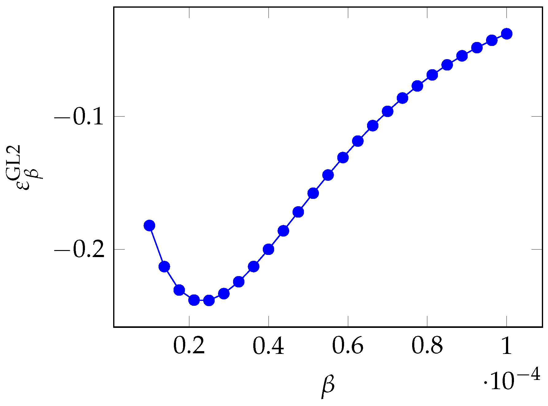
In
Figure 12, we see that the elasticity is not monotone and exhibits a negative peak (which, by the sign of the quasi-elasticity, implies the maximum influence), slightly above
in the picture.
By exploiting the very same breach probability function of Equation (
4), we can derive that
and rewrite the quasi-elasticity as
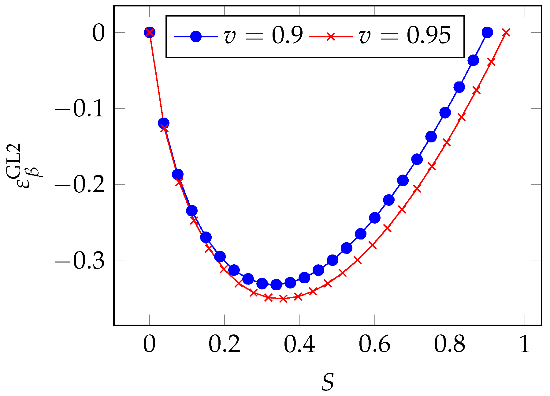
By taking a look at
Figure 13, we see that the influence of
reaches a maximum for an intermediate value of the breach probability. Precisely, we have the maximum influence when
, i.e., when the breach probability is reduced to
. The correct estimation of
is then least critical when the investment is either small or large (which means that the reduction in the breach probability is, respectively, minimal or so large as to be beyond the
factor).
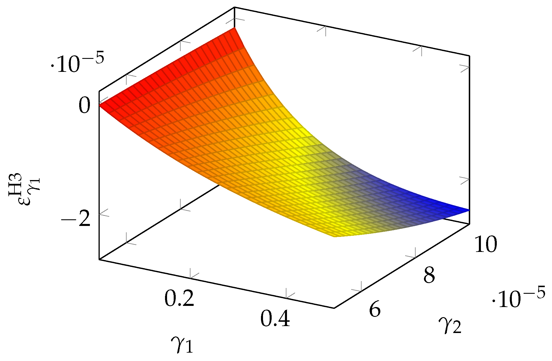
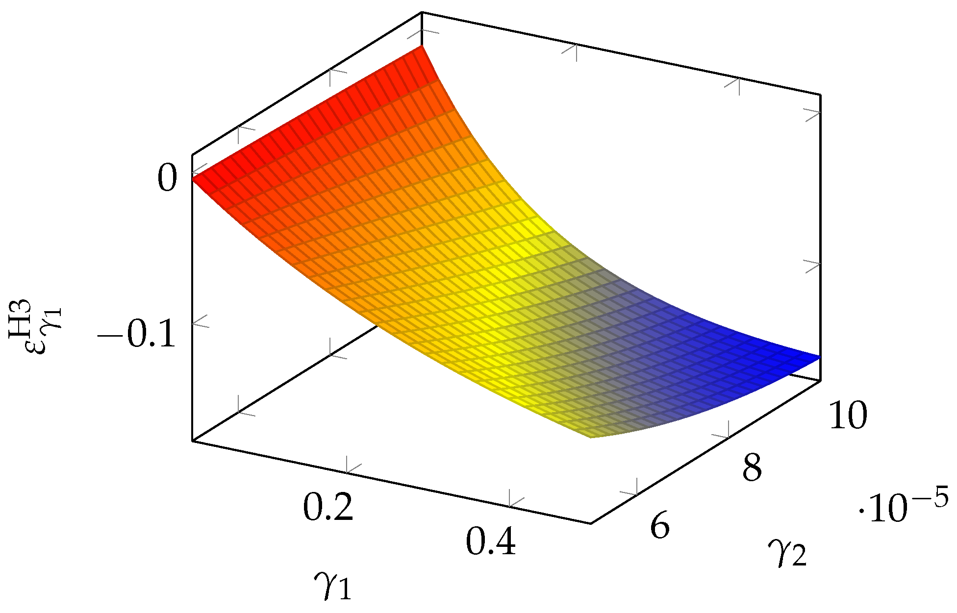
3.4. Hausken Class Three Model Elasticity
With the Hausken Class Three model, described in
Section 2.5, we return to a two-parameter model such as the GL1. The two parameters are here named
and
. After recalling the definition of Equation (
4), we can compute the quasi-elasticity for
, which is
The relative relevance of the two parameters follows what we have already seen for the GL1 model. In
Figure 14, we see that the sensitivity to
is quite driven by
itself and becomes heavier when
grows.
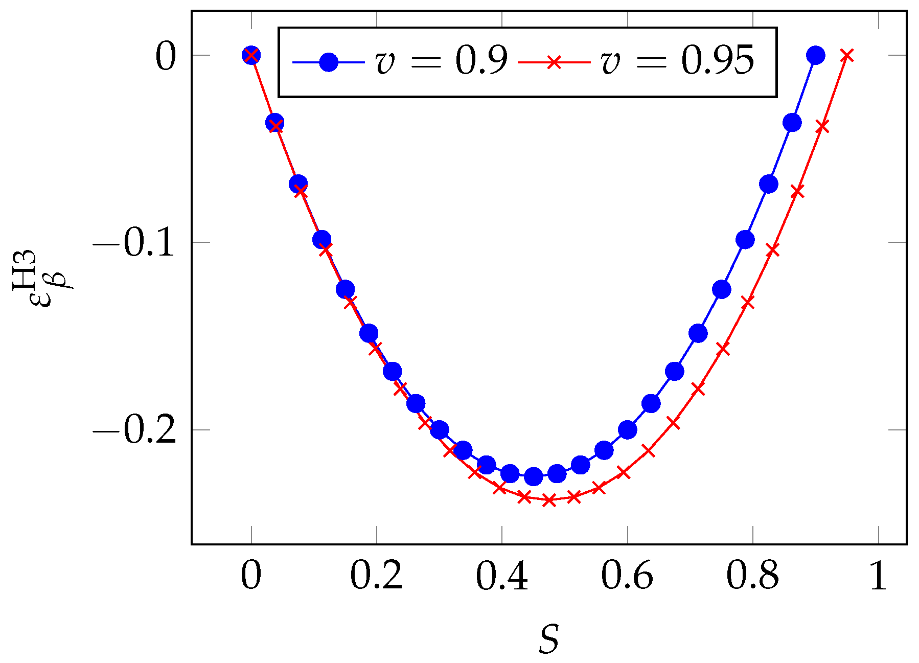
We can also analyze the regions of greatest sensitivity by rewriting Equation (
22) as a function of the breach probability
S. After a few algebraic manipulations, we obtain
which is plotted in
Figure 15 for two values of the a priori vulnerability
v. As observed in the Gordon–Loeb model, we see that the peak of sensitivity occurs for intermediate values of the breach probability (between 0.4 and 0.6). We can obtain the precise location of the peak by zeroing the derivative
which gives us
The maximum influence of
on the breach probability function
S is reached when the investments are such as to reduce the vulnerability by half.
If we turn to the second parameter, we obtain the quasi-elasticity
which is plotted in
Figure 16. We see that
is most influential when both parameters are large.
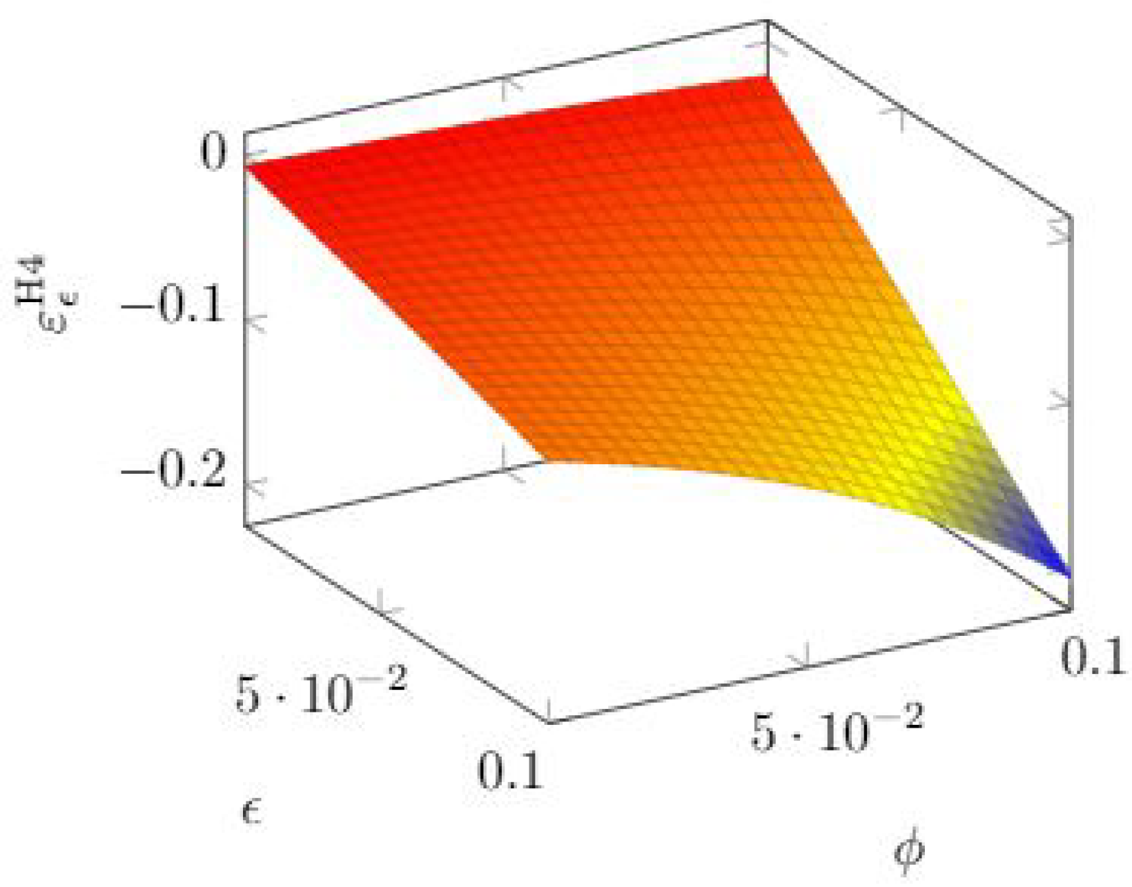
3.5. Hausken Class Four Model Elasticity
Here, we have another two-parameter model. The parameters are now , not to be confused with the symbols used for the quasi-elasticity, which is always accompanied by the variable, the model, and .
By recalling the definition of the breach probability function in Equation (
6), we have
We have a negative quasi-elasticity again for both parameters, excepting the regions where the quasi-elasticity is null because the breach probability function is null itself (actually, the model validity stops when , since the mathematical expression would lead to a negative breach probability function).
We examine first the sensitivity with respect to
. In
Figure 17, we see that the sensitivity to that parameter grows with both parameters in such a way that keeping either parameter very low makes the breach probability function nearly inelastic to
.
We can also find for which investment range the choice of
may be more critical. If we use the breach probability function definition in Equation (
6), we obtain
, so that the quasi-elasticity can be expressed as
A linear relationship appears, which means that the sensitivity to is very small when investments are small (so that the reduction in vulnerability is itself small) but gradually grows when investments increase.
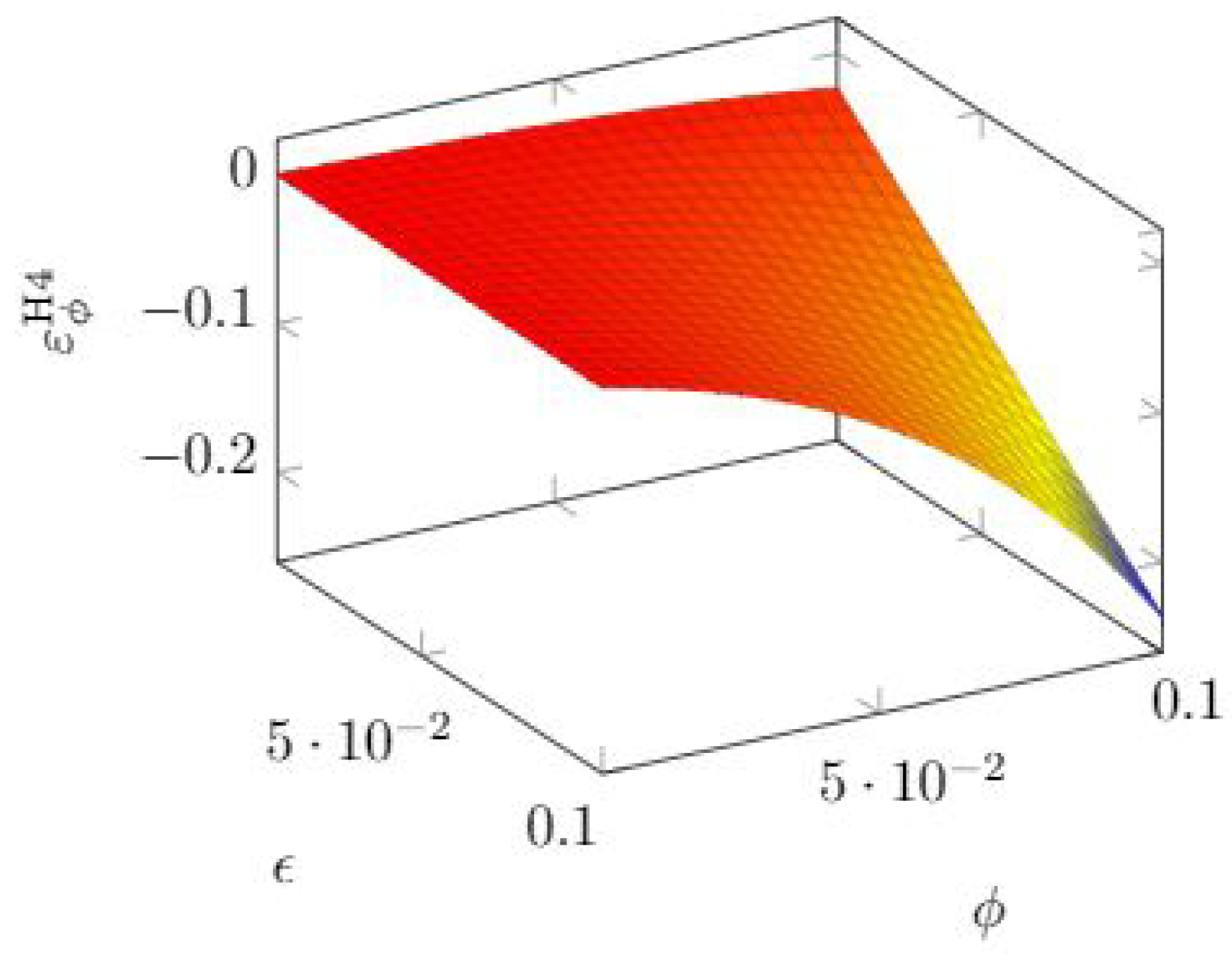
If we turn to the effect of
, we see similar behavior in
Figure 18: the quasi-elasticity becomes significant when both parameters grow.
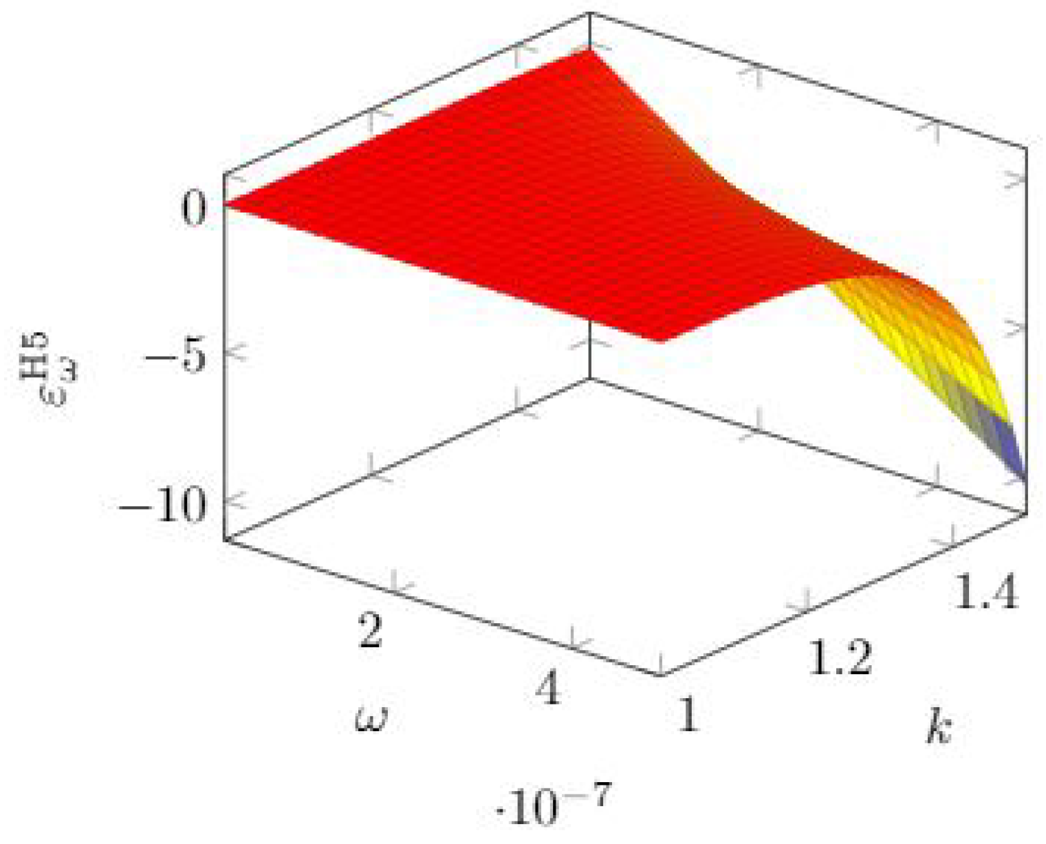
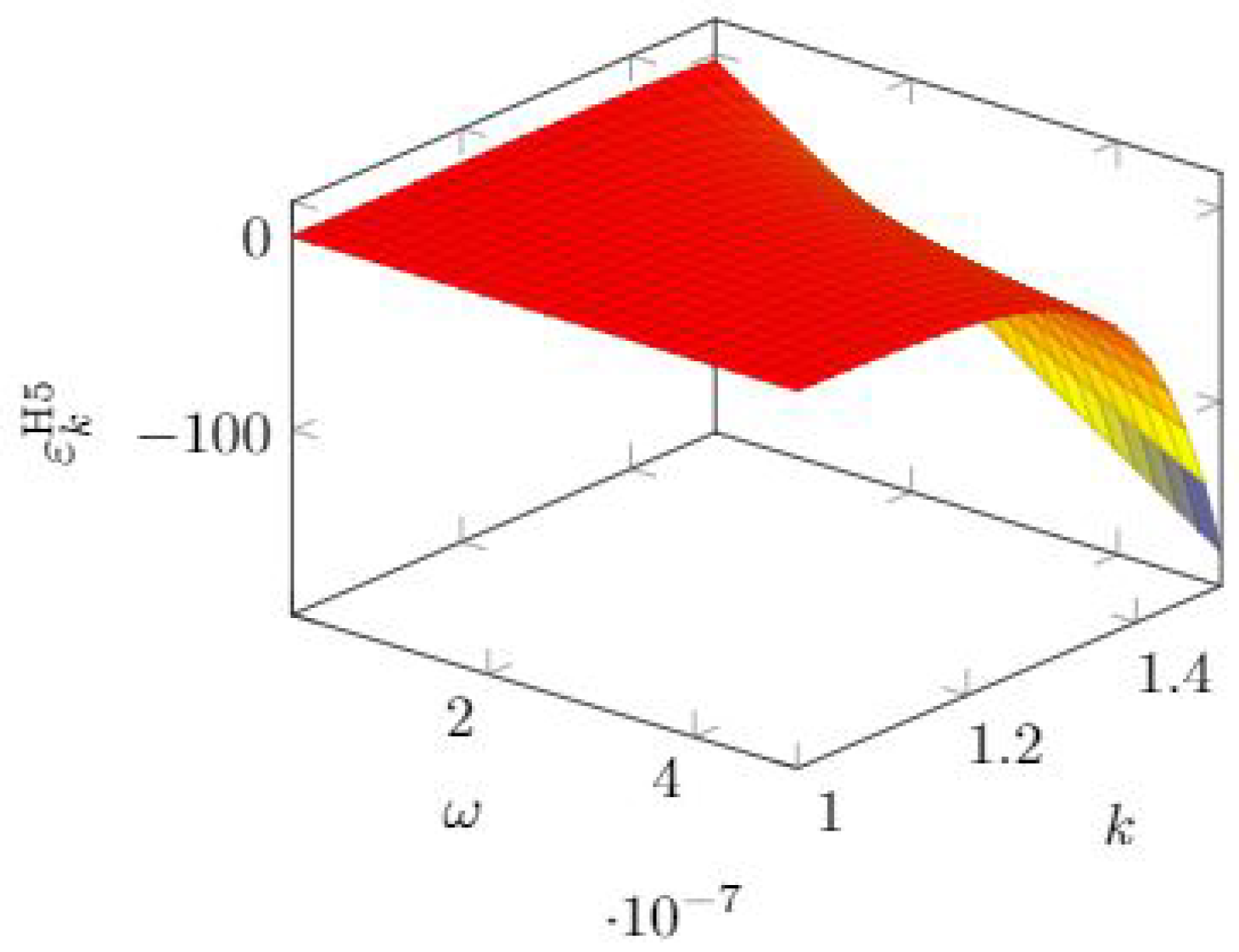
3.6. Hausken Class Five Model Elasticity
As shown in
Section 3.6, the H5 model has the same mathematical expression as the H4 model, but they differ in the parameter range for
k. Hence, we obtain the same expression for the quasi-elasticity. Since the models assume that we can reach complete invulnerability, the limiting value for the investment
is due to the mathematical need to avoid negative values for the breach probability. The expressions for the quasi-elasticity are then
In
Figure 19, we see that the sensitivity to
grows rapidly when the other parameter
k exceeds 1.2 roughly and
is itself in the higher range (
roughly).
Quite a similar behavior is observed for the quasi-elasticity with respect to
k, as can be observed in
Figure 20.
Given the identity of the mathematical expressions of the breach probability function of the H4 and H5 models, we can write the quasi-elasticity with respect to
as
which shows again a linearly growing sensitivity when the breach probability reduces due to larger investments.
3.7. Hausken Class Six Model Elasticity
We consider here what is probably the simplest breach probability model, described by the linear relationship with a single parameter (
) shown in Equation (
8).
The computation of the quasi-elasticity gives us again a linear function:
The quasi-elasticity function is amenable to be expressed as a function of the breach probability function. After a few simple manipulations, we obtain again, however, a linear function, as we did for the H4 and H5 models:
Hence, the impact of the parameter is stronger when investments are so large as to reduce the breach probability down to low values.
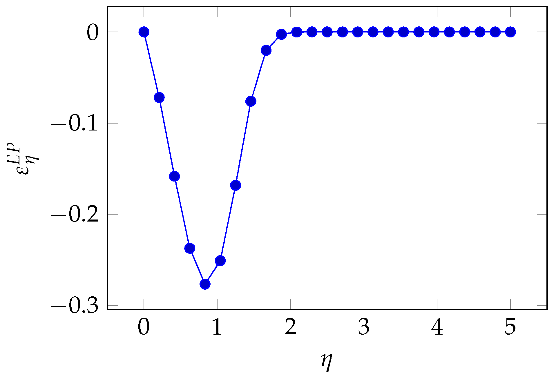
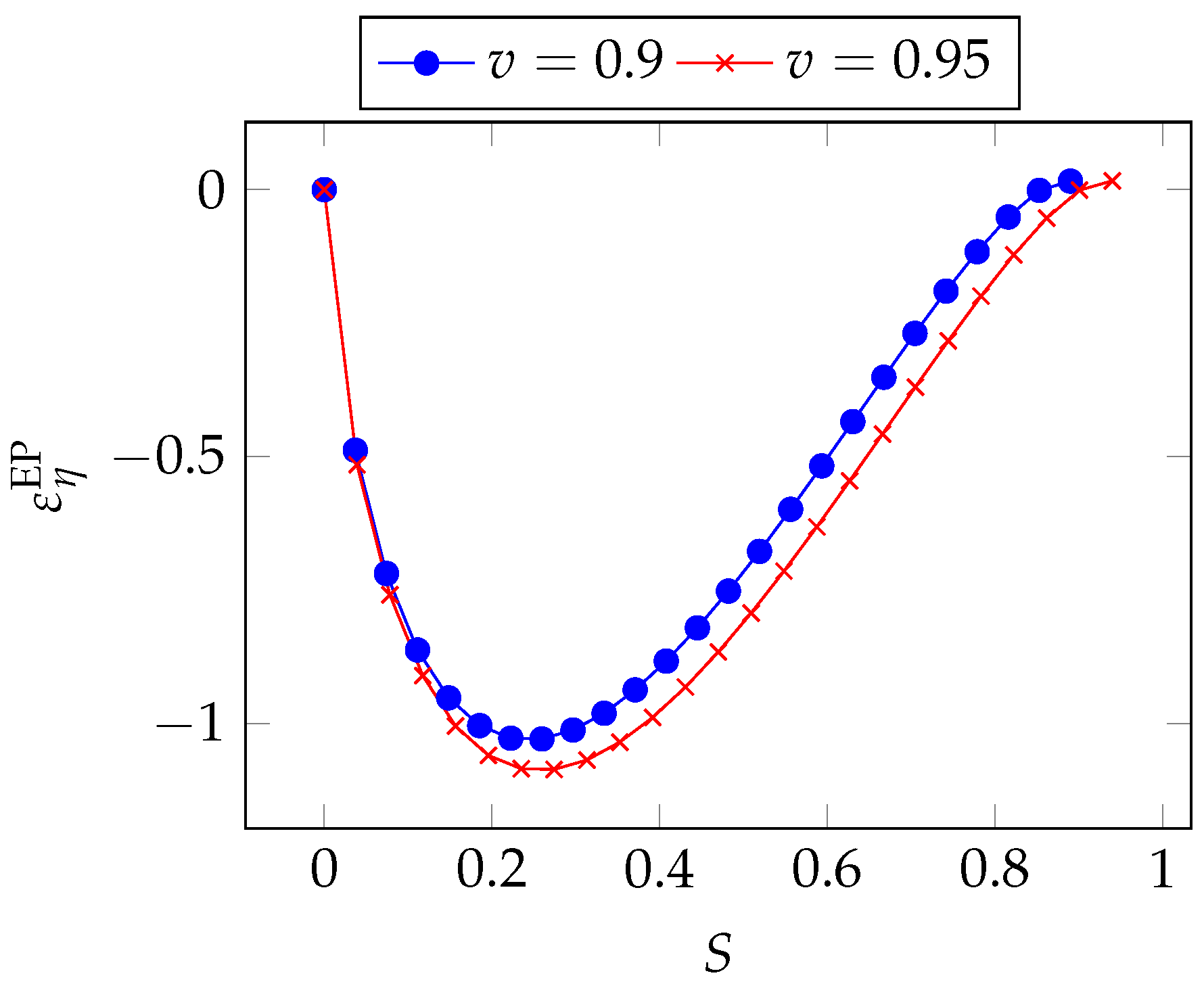
3.8. Exponential Power Class Elasticity
If we write the breach probability function as
where
is the breach probability obtained when the investment equals some benchmark value
B, we can compute the quasi-elasticity with respect to the exponent
.
After a few algebraic manipulations, we obtain
In
Figure 21, we see again the pattern where the sensitivity is higher for intermediate values of investments. If we push investments still further to reduce the breach probability, the influence of
goes down till becoming negligible.
We can also analyze the regions of greatest sensitivity by rewriting Equation (
36) as a function of the breach probability
S. We first derive the following relationship by taking the logarithm of both sides of Equation (
35):
After some algebraic manipulation, we obtain
In
Figure 22, we see the same pattern as in the GL2 model, though a significant asymmetry is observed here, with the maximum influence taking place for lower values of the breach probability.
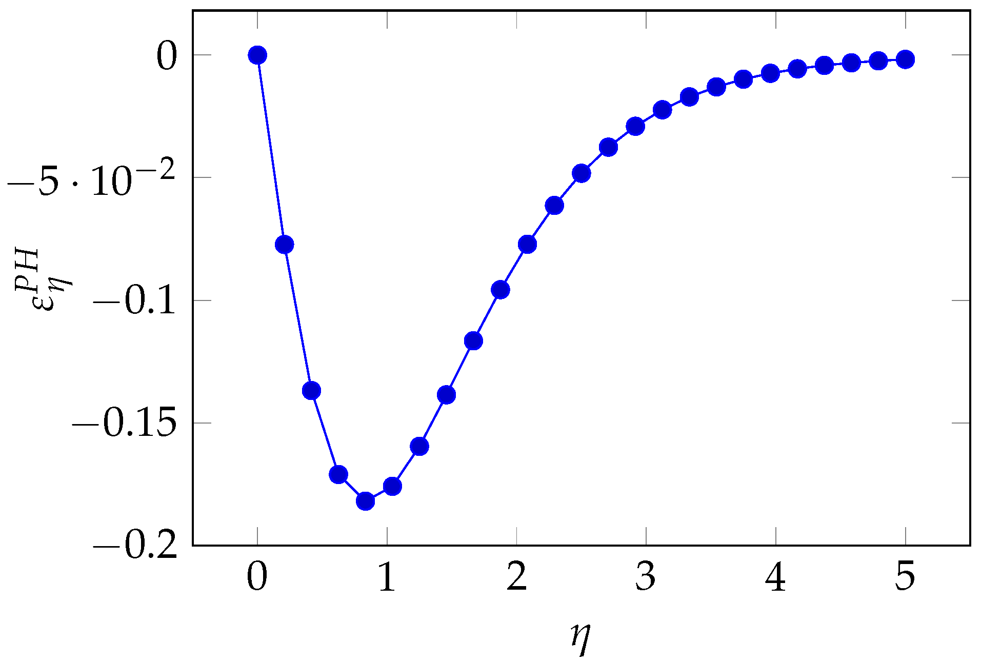
3.9. Proportional Hazard Class Elasticity
Here, we have again a two-parameter model, whose breach probability function is reported as Equation (
12). First, we obtain the quasi-elasticity with respect to the parameter
as
The resulting function is plotted in
Figure 23, where we observe a pattern similar to that of the Exponential Power Class, i.e., the greatest sensitivity for intermediate values of the parameter
.
If we write the breach probability function in its original form
where
is the breach probability function when the investment
z equals the benchmark value
B, we can derive the following relationship, which proves useful to express the quasi-elasticity in a suggestive way:
By exploiting this relationship and recalling Equation (
39), we obtain
In
Figure 24, we find the same trend as in the Exponential Class.
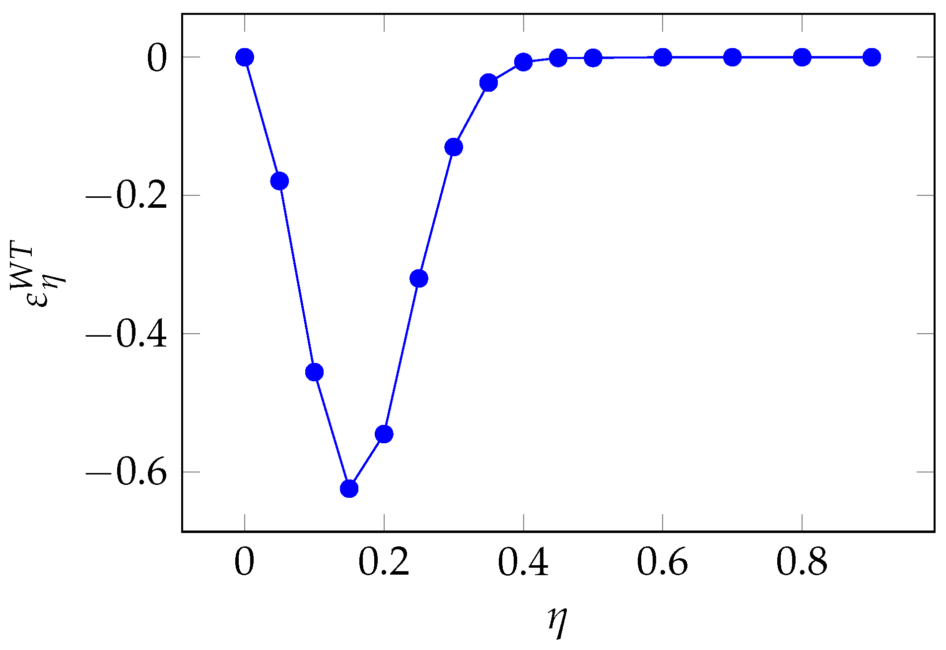
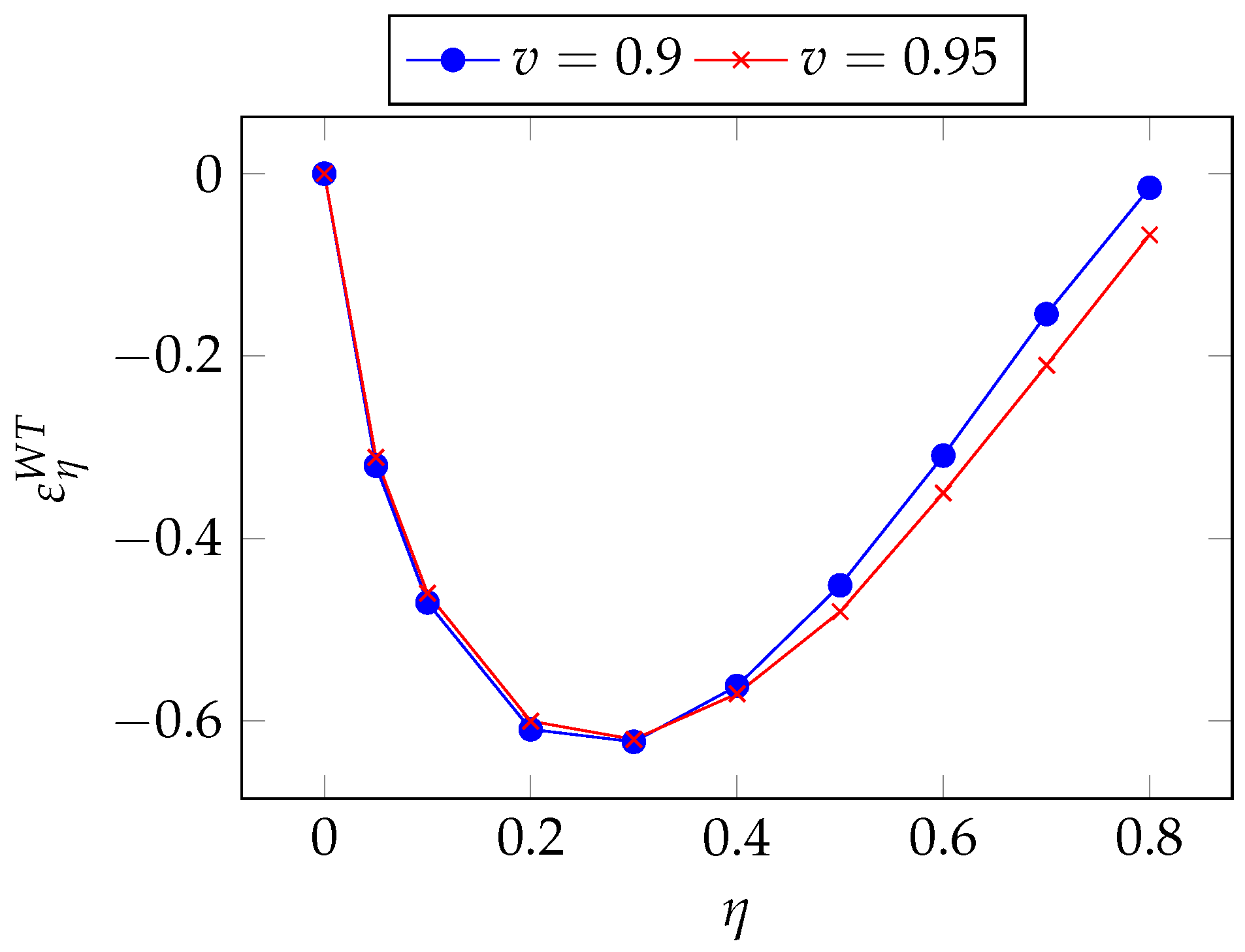
3.10. Wang Transform Class Elasticity
Finally, we conduct the same analysis for the Wang Transform model, which is a two-parameter model. As in the EP and PH models, however, we focus on
. The pertaining quasi-elasticity is
We find the same pattern as seen for the EP and the PH model, i.e., a peak of sensitivity followed by a fast retreat to zero sensitivity as
grows, as can be observed in
Figure 25.
If we write the breach probability function as
we find the following relationship:
which proves useful to express the quasi-elasticity as a function of the breach probability.
In
Figure 26, we see a trend again similar to what we found in the EP and PH models.
4. Conclusions
We provided a presumably complete view of the breach probability functions proposed in the literature to model the effect of cybersecurity investments on the actual vulnerability to cyberattacks. The variety of forms taken by these functions allows us to be reasonably confident that they can be used to fit many contexts adequately.
We can take different approaches to compare them and choose what is probably the best for us. In this conclusion, we examine all of them.
First, we can examine the properties they exhibit. In
Table 3, we report how the different models comply with the properties we set in
Section 2.2. We notice that all models exhibit Properties
through
, i.e., all models assume that investing in security does always improve the robustness of the system till the point of turning mitigation into a nearly complete shield against attacks. However, they differ in the additional impact that further investments get. We have just one model (H6) assuming that returns on investments are linear: the same additional investment leads to the same vulnerability decrease, regardless of the initial situation. All other models assume that the impact of further investments depends on the starting point. Both the models by Gordon and Loeb and the Hausken Class Four consider diminishing returns, which inevitably leads to a point after which it does not pay to invest more in security. On the other end of the spectrum, we have the Hausken Class 5, which implies a snowball effect: we obtain a more-than-proportional reduction in vulnerability by investing more. In between, all other models (H3, EP, PH, and WT) predict a strong initial reduction in vulnerability, followed by diminishing returns.
A major element to assess the importance of those models is their usage. In the literature, we found applications reported for the GL1, GL2, H3, PH, and WT models. Aside from their proponents, we did not find applications of H4 through H6, or EP models, which have yet to prove their relevance.
An additional way to compare them is to look at the complexity of the model, as embodied by the number of parameters. This is actually a two-sided argument. When the number of parameters grows, we obtain more parameters to estimate, but the model becomes more flexible at the same time. Anyway, in the array of models we examined, the number of parameters is two at most. We have three models that are fully characterized through a single parameter: Gordon–Loeb Class 2, Hausken Class 6, and Wang Transform. All other models have two parameters. In the case of two-parameter models, one is typically more critical than the other, since their influx on the overall breach probability is larger, requiring more attention in their estimation.
A fundamental limitation of the models presented here is that they are all derived from first principles. A strong trend in risk analysis is the shift to a more data-centric approach
Aven and Flage (
2020), as underlined by
Ale (
2016),
Choi and Lambert (
2017), and
Nateghi and Aven (
2021). Unfortunately, data are still scarcely available in the cybersecurity world. In addition, the models should be developed using a counterfactual approach, comparing the outcome of the investments in cybersecurity with what would have happened if no investments were carried out. An attempt to calibrate a security breach probability function by relating the investment with the resulting vulnerability has been proposed in
Naldi and Flamini (
2017).
In addition, all the current models are of the one size fits all kind. They do not differentiate among cybersecurity countermeasures: an investment in a firewall is considered as valuable as an investment of the same amount in antivirus software or one in cybersecurity education. The time has come to progress towards a finer description of the return on security, considering the different possibilities that a cybersecurity officer has.
Though the current models have opened the path to a greater awareness of the economic trade-offs of investing in security, the increase in spending, dictated by the growth of cyberthreats, calls for more careful investment decisions, which in turn requires more accurate models if they have to become operational tools rather than just indicative.
[custom] References


