Abstract
This paper proposes a two-step LASSO based vector autoregressive (2-LVAR) model to forecast mortality rates. Within the VAR framework, recent studies have developed a spatial–temporal autoregressive (STAR) model, in which age-specific mortality rates are related to their own historical values (temporality) and the rates of the neighboring cohorts (spatiality). Despite its desirable age coherence property and the improved forecasting accuracy over the widely used Lee–Carter (LC) model, STAR employs a rather restrictive structure that only allows for non-zero cohort effects of the same cohorts and the neighboring cohorts. To address this limitation, the proposed 2-LVAR model adopts a data-driven principle, as in a sparse VAR (SVAR) model, to offer more flexibility in the parametric structure. A two-step estimation strategy is developed accordingly to resolve the challenging objective function of 2-LVAR, which consists of non-standard L2 and LASSO-type penalties with constraints. Using empirical data from Australia, the United Kingdom, France, and Switzerland, we show that the 2-LVAR model outperforms the LC, STAR, and SVAR models in most of our forecasting results. Further simulation studies confirm this outperformance, and analyses based on life expectancy at birth empirically support the existence of age coherence. The results of this paper will help researchers understand the mortality projections in the long run and improve the reserving/ratemaking accuracy for life insurers.
1. Introduction
With the ongoing increase of life expectancy around the world, mortality modeling and forecasting have become essential for measuring mortality and longevity risks. In actuarial research, mortality risk is generally regarded as the risk of financial losses caused by people living shorter than expected, whereas longevity risk is caused by people living longer than expected. There can be several factors driving continual mortality improvements, for example, advances in medical science, innovative improvements in technology, and changes in lifestyle. Forecasting mortality rates has become an important task in demographic research and also in the insurance industry. For the latter, the worldwide mortality improvements have significant impacts on pension funds as well as policymakers. Unreliable mortality forecasts can lead to inaccurate pricing and reserving and so greater insolvency risks. Accurate mortality modeling and forecasting methods are very much needed in assessing mortality and longevity risks.
Among the existing methods to study and forecast mortality rates, the Lee–Carter (LC) model (Lee and Carter 1992) can be considered as the most widely used factor-based model. Please see Renshaw and Haberman (2006) and Cairns et al. (2006) for other related seminal work. More recent developments of such models include He et al. (2021). Studies such as Perla et al. (2021), Richman and Wüthrich (2021), and Wang et al. (2021) have considered machine learning extensions of the LC model. Despite their popularity, factor-based models have certain limitations, such as identifiability (Hunt and Blake 2018) and the lack of age coherence. More specifically, age coherence is defined as the condition that forecast mortality rates will not diverge between any two ages in the long run, and it is a desirable feature from the perspective of biological reasonableness (Li and Lu 2017). To tackle these issues, vector autoregressive (VAR) models have been proposed, with a major advantage of having more flexible temporal modeling of mortality rates (see, for example, Chang and Shi 2021, 2022a, 2022b; Guibert et al. 2019; Yang and Wang 2013, among others.) In this study, we take a step further and propose a two-step LASSO based VAR (2-LVAR) model, and this new approach represents a significant contribution to the expanding family of VAR-type mortality models.
The current VAR models deal with two major challenges of modeling mortality rates: the high dimensionality (i.e., the large number of ages relative to the number of years) and the non-stationarity (i.e., consistent temporal reductions). For instance, the influential work of Li and Lu (2017) proposed a spatial–temporal VAR (STAR) model with pre-determined sparsity and imposed equality constraints on the coefficient matrix. Consequently, the STAR model has a small number of unknown parameters that can be estimated ordinarily and is a co-integration1 system that overcomes the non-stationarity problem. The co-integration also ensures the desirable age coherence property. However, the sparsity of coefficients of STAR is rather ad-hoc. As an alternative, Guibert et al. (2019) took a data-driven approach and developed a sparse VAR (SVAR) model with its estimation conducted via the widely known elastic-net (ENET) algorithm. To resolve the non-stationarity problem, however, the SVAR model needs to work with mortality improvements (differenced rates) instead. Consequently, although the SVAR model may improve the performance of mortality forecasting in some cases, the age coherence property is lost under the SVAR model (Li and Lu 2017).
Based on the STAR and SVAR models, recent studies have explored different extensions. Chang and Shi (2020) employed the STAR specification within a time-varying parametric framework. Feng et al. (2021) adopted the hyperbolic decay to allow for more flexible sparsity in the coefficient matrix, whereas Shi (2021) enabled this sparsity by considering sample correlations among age-specific rates. Chang and Shi (2021) incorporated smoothness penalties to the SVAR model and constructed a smoothed SVAR (SSVAR) model, which ensures the age coherence property asymptotically.
In this paper, the proposed 2-LVAR model is a new and more effective approach to combine the merits of the STAR and SVAR models. It also significantly improves upon many recent VAR extensions for forecasting mortality rates. In short, we adopt the framework of Chang and Shi (2021) but work with the undifferenced mortality rates. This setting ensures age-coherent forecasts without requiring that the sample size grows asymptotically, and significantly improves the SSVAR model. The parameter estimation, however, is not straightforward, as the framework requires equality constraints, as in the STAR model. To cope with this technical difficulty while maintaining ease of implementation, a two-step estimation strategy is devised. In the first step, we eliminate the equality constraint via substitution and fit the unconstrained model using a usual LASSO algorithm with age-adaptive weights. The data-driven sparsity in the coefficients is then obtained. In the second step, we employ the penalized least squares (PLS) as in the STAR model to accommodate the smoothness penalties.
To demonstrate the effectiveness of our proposed model, we provide empirical evidence using the mortality rates of four countries: Australia, the United Kingdom, France, and Switzerland. All data are sourced from the Human Mortality Database (2021), and the forecasting performances of the LC, STAR, SVAR, and 2-LVAR models are systematically compared on ages 0–100 using the crude unisex rates from 1950 to 2016. Taking the root mean squared error (RMSE) as the forecasting performance measure, we show that the 2-LVAR model consistently outperforms the LC, STAR, and SVAR models when the 1950–2000 subset is employed as the training sample and up to the 16-step-ahead forecasting horizons (2001–2016) are considered. The robustness of our results is further verified by conducting simulation studies. Finally, the age coherence and improved forecasting accuracy of the 2-LVAR model is further supported by an analysis of life expectancy at birth over the period of 2001–2050.
The contributions of this paper are three-fold. First, the proposed 2-LVAR model significantly complements the influential studies of Li and Lu (2017) and Guibert et al. (2019), as well as their recent extensions. In particular, the age coherence property of 2-LVAR addresses the current problem of the SVAR model. As for the SSVAR model, the age coherence feature under our model strictly (rather than asymptotically) holds, which is also more suitable for mortality data with limited sample size. The sparsity of coefficients determined by the LASSO () penalty is more flexible than those studied in Feng et al. (2021) and Shi (2021). Second, the employed two-step estimation process successfully resolves the technical difficulty in fitting our rather complex specification. The LASSO-based estimation in the first step is well developed, whereas the estimation in the second step has a closed-form solution, being the same as under the STAR model. Thus, the overall estimation procedure is computationally efficient. The desirable asymptotic behavior and limited-sample performance are also briefly demonstrated and discussed for those two-step estimators. In our simulation studies, via simulation evidence, the computational cost of 2-LVAR is at a similar level compared to the STAR and SVAR counterparts. Third, we systematically study the forecasting performance of the 2-LVAR model for mortality data of four different countries. Its outperformance over the LC, STAR, and SVAR models indicates the effectiveness of our method to model and forecast mortality rates. Moreover, like the STAR, SVAR, and SSVAR models, the proposed framework can be readily extended to accommodate multi-population modeling. This extension would provide unique information about the cross-population properties and can ensure coherent (non-diverging) forecasts across both ages and populations.
The remainder of this paper is organized as follows. In Section 2, we describe the STAR and SVAR models and briefly explain their drawbacks and also those of recent extensions. We specify the 2-LVAR model and discuss relevant technical details in Section 3, including the statistical properties and estimation procedure. In Section 4, we conduct empirical and simulation studies. Finally, Section 5 concludes this paper and highlights future areas of research.
2. Existing VAR Models
The expanding family of VAR mortality models are attracting increasing attention and provide a sound alternative to traditional factor-based models in the field of modeling and forecasting mortality rates. Compared to those factor-based models such as LC, VAR models offer more flexibility in the specification of the temporal structure, and would capture time, age, and cohort dependencies of mortality data more adequately, without normalization constraints (Guibert et al. 2019; Li and Lu 2017). In addition, when certain parameter constraints are imposed, VAR models can lead to coherent projections between ages and/or between populations. A typical VAR(1) model has the following specification:
where = is the age-specific logged central mortality rates vector (), = is the intercept, is the coefficient matrix, also known as the Granger causality matrix, and = is the vector of error terms. The sample size is denoted by T.
However, there are two outstanding issues in employing a VAR model to study mortality data as discussed in the literature (Shi 2021):
- To produce meaningful estimates and forecasts, the VAR process has to be stationary. However, mortality rates are usually treated as following a non-stationary process in the literature, due to their declining trends over time.
- Under a standard VAR framework, there are often more unknown parameters than observations for mortality data. Consider a VAR(1) model for N age groups. For of each age x, all N lagged log mortality rates need to be considered. Hence, the total number of unknown parameters to be estimated is , which includes N intercepts. Since the number of years T is usually small (dozens), the issue will arise even for an intermediate size of N such as 50. The sign indicates that the number of unknown parameters is much greater than that of observations. This issue is particularly relevant in life insurance practice.
Two pioneering approaches have been proposed in the literature that attempt to address these issues in VAR models. Li and Lu (2017) designed the STAR model with a restrictive coefficient matrix. The restriction focuses on the cohort effects and essentially only allows mortality rates of neighboring ages to interact. To modify this rather ad-hoc structure, Guibert et al. (2019) employed the SVAR model with an ENET penalty estimation method. The SVAR model uses a pure data-driven method to forecast mortality rate improvements within a high-dimensional VAR framework.
2.1. The STAR Model
The STAR model allows for the cohort and period effects in mortality modeling. To deal with the stationarity issue, the STAR model employs an equality constraint in the coefficient matrix such that there is co-integration on the temporal dimension. To reduce the dimensionality of p, STAR applies the sparse spatial information for the age groups. Specifically, Li and Lu (2017) imposed an ad-hoc sparse structure on the coefficient matrix to restrict the number of non-zero parameters.
Considering the VAR(1) model given in Equation (1), the specification of STAR model is provided below:
where , and . The error terms are assumed to follow a multivariate Gaussian distribution with mean vector () and variance–covariance matrix (). The coefficient matrix is constrained such that
In other words, the parameters in each row sum up to be 1 exactly. According to Li and Lu (2017), this constraint ensures a co-integrated system, which is stationary to carry out the further estimation.
The elements in defined above provide direct interpretations of the period and cohort effects. This property can be considered as one benefit of applying VAR-type models in mortality modeling. Specifically, the diagonal components of represent the period effect that captures the impacts of lagged mortality rates of the same age. The sub-diagonal components represent the effects of different cohorts. As defined in Equation (2), is the cohort effect of the same cohort, whereas is the cohort effect of the next younger cohort.
As proved by Li and Lu (2017), by ensuring that all rows of sum up to 1 (the equality constraint), the specification of the STAR model has co-integration and thus resolves the stationarity issue. Specifically, for all neighboring age pairs, and are co-integrated with the order (1,−1). In other words, although is assumed non-stationary for , will be stationary for . Therefore, forecast rates of neighboring age groups will not diverge in the long run and are age coherent. Moreover, as the total number of parameters becomes , which is usually much smaller than , it enables the estimation of VAR. The forecasting is performed in an iterative fashion as follows:
Further, the PLS objective function is used to estimate the parameters. Quadratic smoothness penalties are imposed to reduce the randomness in estimates caused by small sample sizes of mortality data (Li and Lu 2017). Specifically, the following objective function is used in the estimation of STAR model:
where and are norm for a vector and Frobenius norm for a matrix, respectively. In addition, the matrix is defined as below:
Essentially, the smoothness penalties involving and in the above function are non-standard -type penalties. They aim to reduce the irregularities over neighboring elements in
and neighboring rows of , which would be caused by randomness due to small sample sizes of mortality data (Li and Lu 2017). The larger and are, the smoother the estimates will be.
One major drawback of the STAR model is the ad-hoc structure assumed in (2). The non-zero constraints can cover only the cohort effects of the same cohort and the next younger cohort. They cannot accommodate the cohort effects of younger or older cohorts. Moreover, the STAR model ignores the possible differences in the sparsity of Granger causality matrix between different populations.
Based on the STAR framework, Feng et al. (2021) and Shi (2021) suggested two modifications to allow for more flexible sparsity in . Feng et al. (2021) set the effect of younger cohorts to reduce hyperbolically, whereas Shi (2021) used the sample correlation for this decay rate. Despite the improved flexibility, there are two remaining issues. First, the older cohorts (super-diagonals in ) are treated as immaterial with 0s. This structure is still ad-hoc and may not be applicable for all populations. Second, for computational convenience, the decay rates in Feng et al. (2021) and Shi (2021) are set the same across all age-specific mortality rates. This assumption is inflexible compared to the alternative of using age-specific decay rates.
2.2. The SVAR Model
As previously discussed, the issue of makes it infeasible to estimate the VAR model via the usual least squares method. Recall that the sign indicates that the number of unknown parameters is much greater than that of observations. In the general econometrics content, one potential solution is the SVAR model. In the existing literature, the SVAR model has been extensively studied (see, for example, Basu and Michailidis 2015; Fan et al. 2011, among others), and different methods have been explored in shrinking the entries of Granger causality matrix to zero. For instance, one common method is to employ a LASSO-type () penalty to force some coefficients in the Granger causality matrix to become exactly zero.
Regarding the modeling and forecasting of mortality data, Guibert et al. (2019) employed the SVAR model as a pure data-driven approach and an alternative of STAR. There are two major differences compared to the STAR method. First, in order to have stationarity, the differenced mortality rates (), or the mortality improvements, are modeled. Second, instead of the ad-hoc structure in (2), the choices of non-zero entries in are determined by the data. In the matrix form, the specification of SVAR model with lag one is displayed below:
where . The estimation is conducted via the widely adopted ENET algorithm (Zou and Hastie 2005). When only the LASSO penalty is considered, we have the following objective function:
where is the norm or the Euclidean distance of a vector, is the penalty parameter that aims to shrink some of the s to zero and therefore controls the sparsity of matrix.
Note that the initial SVAR model is not tailored to mortality data, and so employing it without suitable modifications may generate questionable results. For instance, the empirical analysis in Guibert et al. (2019) indicated that the mortality improvement at age 95 could still influence the improvement at age 45 (i.e., ), which is not sensible. To overcome this problem, Chang and Shi (2021) employed age-adaptive weights, the details of which will be discussed in Section 3.
A more critical issue of the SVAR model, however, is the lack of age coherence. This problem arises from the fact that there is no co-integration allowed, as a direct consequence of using the mortality improvements. The SSVAR model developed in Chang and Shi (2021) may achieve age coherence, though only asymptotically. This limitation may hinder the performance in mortality forecasting, especially when the training data often have a small sample size.
3. The 2-LVAR Model
In this section, we specify the proposed 2-LVAR model and present the two estimation steps of the model, together with a procedure to select tuning parameters. Statistical properties related to the co-integration and age coherence are also briefly discussed.
3.1. Model Specification
To retain the merits of STAR and SVAR models, it is preferable to work with the original mortality rates via a data-driven approach. The 2-LVAR model is particularly designed to study and forecast mortality in this direction.
With the same model specification expressed in Equation (1), the major difference between the 2-LVAR and STAR models rests on the specifications of Granger causality matrix . The more flexible matrix in the 2-LVAR model is displayed below:
This more flexible specification is able to incorporate more complicated patterns in the cohort effects, compared to the recent extensions by Feng et al. (2021) and Shi (2021). To have the co-integration, as in the STAR model, we require the equality constraint for all . Further, we follow Chang and Shi (2021) to impose smoothness penalties and employ age-adaptive weights (see below). The former helps reduce the irregularities in parameter estimates due to small sample sizes, whereas the latter recognizes the lessened cohort effects with widened age gaps.
The aim of setting age-adaptive weights, denoted by for all , is to penalize differently by when estimating the non-zero entries in . The rationale is that the mortality rates at a particular age i are more correlated to those of ages closer to i, compared to those of ages far away from i (Shi 2021). Hence, for larger , should more likely be shrunk to zero or should be more penalized in the objective function. Accordingly, Chang and Shi (2021) defined as follows:
where is the absolute distance between two ages i and j, and is a tuning parameter that controls the sensitivity of shrinkage to the distance between i and j. According to Chang and Shi (2021), the choice of is confounded with the penalty and may be specified by the user rather than estimated from the data. As will be shown in Equation (6), the value of and the penalty term have a confounding impact on the loss function. Thus, it is adequate to fix the value of and select only as the tuning parameter. In this study, we follow Chang and Shi (2021) and let .
It is worth noting that other than the exponential function to derive , methods such as the Matérn family (Cressie and Wikle 2015) may also be adopted, which requires more rigorous computations.
3.2. Estimation of the 2-LVAR Model
The estimation of 2-LVAR model is a non-trivial problem. Ideally, based on the discussions in Section 3.1, the objective function of the 2-LVAR model may be constructed from those of the STAR and SVAR models jointly. Following Chang and Shi (2021), together with the adaptive weights, it may be stated as below:
where and are defined in (3) and (4), respectively, and we constrain that for all and . As stated in previous research such as Li and Lu (2017), those constraints are imposed to ensure the stationarity of the VAR system. A formal proof is given at the end of this section.
The challenge of the estimation is the need to deal with the equality constraint and smoothness penalties at the same time. Note that under the non-standard form of the smoothness penalties, even without the equality constraint, the objective function cannot be solved using the ENET algorithm. Incorporating the equality constraint further complicates the computation. To resolve this technical problem, we split the estimation (objective function) into two steps (parts), where each step (part) can be efficiently computed. In short, we convert the optimization into an unconstrained LASSO exercise in the first step and solve the PLS with a closed-form solution in the second step.
In the first step, the aim is to locate the non-zero elements of the matrix using adaptive weights . With a pre-determined , one then needs to minimize the objective function given below:
where is defined in (4), and we constrain that for all .
To accommodate the equality constraint without increasing the computational burden, this constraint may be eliminated via substitution. Without loss of generality, consider the first age with the following specification:
Under the constraint , we can write . Now, we substitute this in Equation (7) and obtain
Then, for ages spanning 2 to N, we have that
Letting for all we can rewrite (6) as follows:
With pre-determined and , it becomes an unconstrained LASSO problem with weights. Solving it will help identify the locations of non-null in the matrix.
After obtaining the non-zero locations, the second step is to adopt the smoothness penalties to reduce the irregularities in estimates. The optimization problem is now analogous to that of the STAR model, as the sparsity in the matrix is now determined. We can write the objective function for the second step as follows:
Note that if is obtained as in the first step, the corresponding is set to 0 in Equation (10), or otherwise it has to be estimated. In addition, we consider three smoothing parameters: for the intercept , for the temporal effects (diagonal components of ), and for the cohort effects of different ages (all sub- and super-diagonals of ). In this step, we define as a new independent variable that is determined by the estimated in the first step. Specifically, for a given age i, if the estimated , this or otherwise . Since all losses are in quadratic form, for a set of pre-determined smoothing parameters, the optimization follows that for a PLS and therefore has closed-form solution.2
Despite the two-step nature of 2-LVAR model estimation, the proposed strategy is expected to produce asymptotically consistent estimators, under fairly general assumptions. A brief discussion on the assumptions and further simulation results on a small sample (the case of mortality data) are provided in Appendix B.
3.3. Tuning Parameter Selection of the 2-LVAR Model
Altogether, in the 2-LVAR model, there are four parameters that need to be pre-determined and are referred to as tuning parameters: , , , and . Among them, is selected in the first step of parameter estimation, and the rest are selected in the second step. A usual strategy of selecting those tuning parameters is to employ the cross-validation technique. However, the leave-one-age-group-out method is not applicable in our case, because of the time-series nature of mortality data. Therefore, in line with the recent studies of Chang and Shi (2021) and Shi (2021), we employ the procedure known as ‘evaluation on a rolling forecasting origin’ discussed in Hyndman and Athanasopoulos (2018). The selection procedure of in the first step is described below:
- Out of T data points, we use the first 80% as the training sample (i.e., ), where is a function to obtain the integer part;
- For a given , minimize (9) via applying the usual LASSO with adaptive weights on the training sample and obtain 1-step-ahead forecast ;
- Extend the training sample by including one more observation () and repeat step 2 to obtain 1-step-ahead forecast ;
- Repeat steps 2 and 3 until the forecast is generated for all ;
- Calculate the root mean square error (RMSE) value as
Then, the optimum value of can be selected as the value producing the smallest RMSE through a grid search. In this paper, the grid search of is performed over [0.01,0.15].3 With the optimum , we can identify the locations of non-zero entries in . Based on its well-studied features, the LASSO algorithm is computationally efficient.
In the second step and for the remaining three tuning parameters , , and , the same procedure as described above can be followed. Note that the s are selected simultaneously via a grid search. In this paper, we consider the range of [0.01,10] for all three s.4 As discussed above, the loss function in the second step has closed-form solutions. Consequently, despite its two-step estimation nature with four tuning parameters to be selected, our 2-LVAR model is computationally efficient. The computational packages are explained in Appendix A.
3.4. Stationarity of the 2-LVAR Model
In order to maintain the stationarity of the 2-LVAR model, which ensures age-coherent forecasts, the following assumptions will be made on the 2-LVAR model.
Assumption 1.
All series in are time series processes, where indicates the order of integration.
Assumption 2.
Each row of sums up to one. That is, for .
Assumption 3.
The range of all coefficients in is (−1,1).
Assumption 4.
.
Note that Assumptions 1–3 are standard in the existing literature. Particularly, Assumption 1 states that the log mortality rates are considered as non-stationary, as they have a linear long-term trend. Such an assumption is general and widely adopted in mortality literature (see, for example, Lee and Carter 1992; Li and Lee 2005, among others). Assumptions 2 and 3 are technical assumptions. They suggest that the row sum of the Granger causality matrix is equal to one in which each entry of can take values in between −1 and 1. As detailed in Section 3.2, these two assumptions are imposed as parameter constraints in the estimation procedure. Similar assumptions have been made in related literature employing the VAR-type models, such as Li and Lu (2017), Chang and Shi (2021), and Feng et al. (2021). Finally, according to Assumption 4, cannot be rewritten as a perfect linear combination of variables other than in , otherwise is not full-rank. The proposition below summarizes the stationarity property of the proposed 2-LVAR model.
Proposition 1.
Under Assumptions 1 to 4, the difference between any two series of age-specific mortality rates and in the VAR system (1) is stationary for all .
Proof.
See Appendix C. □
The above proposition specifies the stationarity of the 2-LVAR model, and this property ensures the desirable age coherence property in the long run, which are considered as advantages over the LC and SVAR models. Compared to the age-coherent STAR model, we highlight that the proposed 2-LVAR model enables us to examine the cohort effects of mortality rates more comprehensively via a data-driven approach with age-adaptive weights and computational efficiency. Specifically, the data-driven approach replaces the ad-hoc structure of the STAR model, whereas the age-adaptive weights provide more meaningful interpretation of the cohort effects than what SVAR provides. The adopted 2-step estimation procedure successfully tackles the computational difficulty. In the first step, the (unconstrained) LASSO method is well developed and is thus fast to execute. In the second step, the PLS estimation has a closed-form solution with close-to-nil computational cost. These properties ensure the overall computational efficiency of the 2-LVAR model.
4. Empirical Analyses
To demonstrate the effectiveness of the 2-LVAR model, we examine the crude unisex mortality rates of Australia obtained from the Human Mortality Database (2021). Two large European populations of the United Kingdom (UK) and France are also investigated, and the Switzerland data are exploited to check the performance for a small population. To have a reliable and sufficient dataset, we follow Booth et al. (2006) to select an appropriate range of data from 1950 to 2016 covering ages 0–100. The temporal range is to be consistent with recent studies including Guibert et al. (2019), such that the results are directly comparable. The log central mortality rates are plotted in Figure 1. For all four countries, the mortality rates demonstrate consistent improvements over time. Compared with the other three populations, the mortality curves of Switzerland are more irregular with larger variations at ages 0–50, due to the smaller population size.
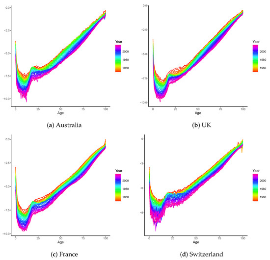
Figure 1.
Logged central mortality rates of Australia, the UK, France, and Switzerland. The datasets include both males and females and span the period of 1950–2016.
In the rest of this study, we split the entire sample into two sub-periods 1950–2000 (training) and 2001–2016 (test). The out-of-sample forecasting performances of the LC (as a widely used benchmark), STAR, SVAR, and 2-LVAR models are systematically compared. Additionally, a simulation study is conducted to check the robustness of our results. Finally, we perform an analysis on the life expectancies at birth over a long period of time.
4.1. Out-of-Sample Forecasting Performance
Consistent with Li and Lu (2017), we adopt the root mean square error (RMSE) to compare the forecasting performances of the LC, STAR, SVAR, and 2-LVAR models. Three RMSE calculations are used in the comparison from different perspectives: RMSE over age groups (), RMSE at individual forecasting horizons (), and the overall RMSE measure (). The definitions of these RMSEs are as follows:
More specifically, is obtained by averaging the RMSE values over all 16 forecasting steps for the age group x. Similarly, to produce , the RMSE values are averaged over all 101 age groups at the time horizon h; is calculated by considering both age and time dimensions up to the step h. The descriptive statistics of are presented in Table 1. Figure 2 and Figure 3 display specific values of and , respectively.

Table 1.
Summary of overall RMSE over age groups.
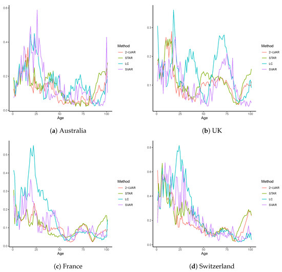
Figure 2.
RMSE over age groups for mortality data of Australia, the UK, France, and Switzerland. The training sample includes 1950–2000, and the test sample includes 2001–2016. The age group includes 0–100. The compared models are LC, STAR, SVAR, and 2-LVAR.

Figure 3.
RMSE over forecasting steps for mortality data of Australia, the UK, France, and Switzerland. The training sample includes 1950–2000, and the test sample includes 2001–2016. The compared models are LC, STAR, SVAR, and 2-LVAR.
In Table 1, we summarize the RMSE values calculated at each age group over all the 16-step-ahead forecasts () of mortality rates of Australia, the UK, France, and Switzerland. For comparison purposes, we also report , the overall RMSE value across all ages and the 16 forecasting steps. The mean, standard deviation (Std. Dev.), first quartile (), and the third quartile () of the are reported. For each population, the numbers in bold indicate the smallest or descriptive statistic values among the LC, STAR, SVAR, and 2-LVAR models. From Table 1, it can be clearly seen that the smallest mean of is obtained from our new model 2-LVAR for all countries. Regarding the variation in performance, the resulting standard deviation under 2-LVAR is among the smallest of all models. It is also worth noting that of produced by 2-LVAR is lower than those of the other competing models in all cases. Therefore, when is examined, our model appears to provide the highest level of average forecasting accuracy with only small variations among ages and no excessively large errors. Similarly, when the overall measure is employed, the 2-LVAR model outperforms the LC, STAR, and SVAR counterparts for all four populations.
Figure 2 provides specific values for all ages. It can be observed that for all countries, the LC and SVAR models may generate very large errors at young ages, especially for those younger than age 50. For the older ages 90–100, however, the STAR model is almost always the worst performing model. This may indicate that the ad-hoc and restrictive structure of (2) could negatively impact the forecasting accuracy at such old ages. Overall, findings consistent with those in Table 1 can still be drawn: of the 2-LVAR model is on average lower than those of the three competing models, with limited variations and no excessively large errors. Thus, employing age-adaptive weights with a data-driven approach would further improve the forecasting accuracy of the STAR framework.
In Figure 3, we plot the RMSE values averaged over all ages () at each individual forecasting step over 1–16 (corresponding to 2001–2016). Distinct differences among all four models are displayed. The LC model often leads to the worst forecasting performance, except for the Australian population. In contrast, the of 2-LVAR model has among the smallest errors at most steps for all countries, suggesting the highest overall accuracy. The differences between the RMSEs of 2-LVAR and those of the other models are more obvious at larger forecasting steps (above 4). In addition, the increment in for the 2-LVAR model is getting lower with the increase in steps compared to the competing models. This result reflects higher forecasting accuracy of 2-LVAR compared to the LC, STAR, and SVAR models in the long run.
Following Li and Lu (2017), to compare the actual and forecast mortality rates visually, we calculate the average mortality rates across ages 0–100 in all four countries. The actual rates over 1950–2016 and the forecast rates over 2001–2016 produced by all four models are illustrated in Figure 4. To further examine the interval results, 95% prediction intervals (PIs) are included in addition to the point forecasts for the proposed 2-LVAR model. Consistent with Li and Lu (2017) and Shi (2021), the PIs are obtained by simulating 1000 scenarios from the multivariate Gaussian distributed errors. That is, the errors are assumed to follow a multivariate Gaussian distribution with 0 means and the variance–covariance matrix equal to the sample variances and covariances5. The h-step forecast is then equal to , where is obtained via the simulation. Overall, it is clear that the point forecasts for the 2-LVAR and STAR models are much closer to the observed values when compared to LC and SVAR for all countries. When considering the interval forecasts, the 95% PIs of the 2-LVAR model cover the observed values satisfactorily over 2001–2016. Moreover, it is worth noting that for the Switzerland data, all the point forecasts of LC and some of SVAR even fall outside the PIs of the 2-LVAR model. The coverage rates of those PIs are studied in next section.
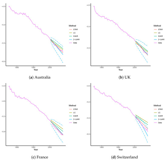
Figure 4.
Forecast vs. actual mortality rates for mortality data of Australia, the UK, France, and Switzerland. The training sample includes 1950–2000, and the test sample includes 2001–2016. The compared models are LC, STAR, SVAR, and 2-LVAR. Presented curves are rates averaged across ages 0–100 for each model or the actual dataset. Dashed lines are the corresponding 95% PIs.
4.2. Simulation Results
To check the robustness of our empirical findings, we conduct a simulation study. Following Feng and Shi (2018), 1000 random scenarios are simulated for all four countries. The true underlying models are assumed to be weighted penalized regression splines with a monotonicity constraint, as described in Wood (1994). This model is often employed to smooth out the crude mortality rates. We take the following steps to produce simulated data for all countries:
- Fit the entire sample over 1950–2000 using the weighted penalized regression splines and calculate the residual errors by subtracting the fitted rates for age x at time t from the observed log central mortality rates;
- Assume a multivariate Gaussian distribution for the collected errors using the sample means and covariances, and simulate errors for each country; and
- Add simulated errors to the fitted values obtained in step 1, and repeat all steps to produce 1000 scenarios.
For each of the 1000 scenarios for all countries, we fit the LC, STAR, SVAR, and 2-LVAR models to produce 16-step-ahead forecasts. Using the observed sample over 2001–2016, the values are then calculated. For each population, we present summary statistics (mean, standard deviation, first quartile , and third quartile ) for these 1000 RMSE values in Table 2.
Table 2.
Summary of simulation results.
Overall, the descriptive statistics displayed in Table 2 are consistent with our previous findings. Despite giving the lowest standard deviations in RMSE, the LC model results in lowest average accuracy. In contrast, being consistent among all countries, our 2-LVAR model produces the lowest mean, , and of the , with relatively small variations. To compare the differences visually, we plot smoothed densities of the RMSEs in Figure 5. For all four countries, the densities generated under the 2-LVAR model are centered to the left end with small standard deviations, and their shapes are roughly a bell curve.
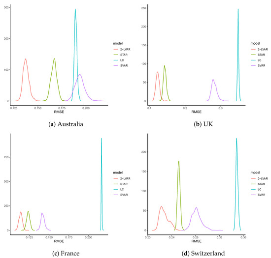
Figure 5.
Density plots of RMSEs of simulated mortality rates of Australia, the UK, France, and Switzerland. The curves are based on smoothed densities produced by the 1000 for each model.
Regarding the computation runtime, the completed estimation of the LC, STAR, SVAR, and 2-LVAR models required 0.03, 0.41, 0.57, and 1.03 seconds, respectively. The runtime is averaged across all replicates and all populations. This result illustrates the computational efficiency of the proposed 2-LVAR model as argued in Section 3. Thus, with marginally increased computational cost, our simulation results demonstrate that overall the 2-LVAR model outperforms the LC, STAR, and SVAR models in terms of the out-of-sample forecasting accuracy.
Finally, we compute the coverage rate of the 95% PIs as explained in Section 4.1. This rate is calculated by considering the proportions that the PIs cover the true values, as plotted in Figure 4. For each previously generated replicate, we compute the 95% PI of mortality rate averaged across all ages over 2001–2016. The proportion of the true values falling within this PI is then recorded. On average, this proportion is 97.7%, 99.1%, 98.7%, and 96.3% for Australia, the UK, France, and Switzerland, respectively. Thus, the interval estimation of 2-LVAR introduced in Section 4.1 provides a reasonable way to construct the PIs.
4.3. Analysis of Life Expectancy over the Long Term
Considering the long-term dynamics, we examine the (period) life expectancy at birth () for each country. Note that the calculation of involves the mortality rates of all ages. Thus, apart from the demographic importance, the analysis of provides insightful information for the mortality dataset under investigation and is particularly useful for a long-term view.
In line with our previous setting, the training sample consists of years 1950–2000. We then forecast the life expectancy at birth up to 2050. To demonstrate the influence of age coherence, we compare only the forecasts of the LC and 2-LVAR models. Figure 6 displays both point and interval forecasts for all the four countries examined. The observed over 1950–2016 and the forecast of the LC and 2-LVAR models over 2001–2050 are plotted. Based on 1000 simulated scenarios, the 95% PIs from the 2-LVAR model are also reported, where errors are assumed to follow a multivariate Gaussian distribution (Li and Lu 2017; Shi 2021).
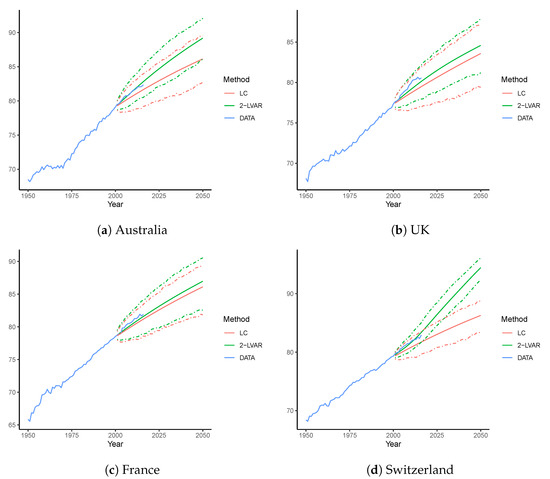
Figure 6.
Forecast life expectancy at birth for Australia, the UK, France, and Switzerland using the LC and 2-LVAR models. The training sample includes 1950–2000. The life expectancy is forecast over 2001–2050. Dashed lines are the corresponding 95% PIs.
For all four countries, it is clear that the 2-LVAR model consistently produces higher mean forecasts of than the LC model. This difference supports the fact that the mortality forecasts of the 2-LVAR model are age-coherent. According to Li and Lu (2017), age-coherent mortality forecasts will lead to higher life expectancy than non-age-coherent forecasts, as the mortality improvements at very old ages are higher for age-coherent forecasts. Over the period 2001–2016, forecast values of from the 2-LVAR model are closer to the observed values than forecast from the LC model in all countries. Further, all the observed values of fall well within the corresponding 95% PIs under the 2-LVAR model. In 2050, for Australia, the UK, France, and Switzerland, point forecast values of obtained from the 2-LVAR model are 89.2, 84.6, 87.0, and 91.5, respectively, and those obtained from LC model are 86.1, 83.6, 86.1, and 86.3, respectively. Nevertheless, the widths of PIs for 2-LVAR are narrower than the LC counterparts. As Section 4.2 has shown evidence on the satisfactory coverage rate of the 2-LVAR PIs, it may be inferred that the interval estimation of 2-LVAR is more efficient than that of the LC model.
In summary, regarding out-of-sample forecasting accuracy, the proposed 2-LVAR model consistently outperforms the LC, STA, R and SVAR models for the populations of Australia, the UK, France, and Switzerland. This outperformance is shown by the RMSE values obtained over ages (), forecasting steps (), and both age and time (). The age coherence property of the 2-LVAR model is demonstrated when life expectancy at birth () over 2001–2050 is forecast for all four countries. Once again, we observe more accurate out-of-sample forecasts of under the 2-LVAR model than under LC over 2001–2016. All our results show that the proposed 2-LVAR model can serve as a powerful and effective tool in forecasting and studying mortality rates for demographic and actuarial research.
5. Conclusions and Future Research
In this study, we proposed a two-step LASSO based vector autoregressive (2-LVAR) model to study and forecast mortality rates. We demonstrated the effectiveness of the 2-LVAR model by considering mortality data of four populations: Australia, the UK, France, and Switzerland for 1950–2016. The following key results highlight the performance and effectiveness of the 2-LVAR model.
First, the 2-LVAR model retains the advantages of both the STAR (Li and Lu 2017) and SVAR (Guibert et al. 2019) models by adopting a more general framework. It resolves the outstanding issues of the recently developed extensions of STAR and SVAR models in Feng et al. (2021), Shi (2021), and Chang and Shi (2021). Specifically, we remove the ad-hoc structure of the Granger causality matrix as in the STAR model and adopt a data-driven approach to select non-zero elements. Compared to the SVAR model, by employing the age-adaptive weights proposed in Chang and Shi (2021), the data-driven approach is more appropriately tailored to mortality data. Second, the proposed 2-LVAR model has attractive technical features. The two-step strategy largely reduces the challenge to accommodate the constrained LASSO with non-standard -type penalties. In each step, the estimation algorithm involved is either well developed (unconstrained LASSO with weights in the first step) or in closed-form (for PLS in the second step). Consequently, the overall computational efficiency of 2-LVAR is at a similar level as the less complicated counterparts STAR and SVAR models and much higher than those of the SSVAR and CSVAR models. Further, working with the equality constraint and undifferenced mortality rates, the desirable co-integration is realized, and thus age-coherent forecasts of mortality rates can be obtained. Third, our empirical analyses demonstrate the improved out-of-sample forecasting accuracy of 2-LVAR over the LC, STAR, and SVAR models. Using a comprehensive dataset of crude unisex mortality rates of Australia, the UK, France, and Switzerland over 1950–2016 for ages 0–100, our 2-LVAR model generally outperforms the three competing models. Simulation results further confirm these findings.
As for future research directions, it is worth exploring ways to address the limitations of the 2-LVAR model. For instance, as shown in Section 4.1, the coverage rate of PIs of 2-LVAR is higher than expected. This result may be attributed to the lower efficiency of the sample variance–covariance matrix when it is used to estimate the population parameters with a small sample size. To overcome this inefficiency, future research may consider the modeled error dependencies as in Li and Lu (2017) and Chang and Shi (2021). Other possibilities include exploring the Bayesian framework to enable more comprehensive parametric structure on the covariance (Li et al. 2019). In addition, this paper focuses on the single-population scenario only. Due to reasons such as global improvement in public health, medical advances, transportation, and technology, the mortality rates of (geographically, socially, culturally, etc.) related populations tend to be (strongly) correlated. Thus, it is worth investigating multi-population mortality modeling. Previous studies such as Li and Lee (2005), Cairns et al. (2011), and Zhou et al. (2014) have made significant attempts on the multi-population mortality modeling to study common patterns in a large group of populations. The extension of VAR-type models to a multi-population framework is usually straightforward, and attempts have been made for the STAR and SVAR models. Following Li and Lu (2017), Guibert et al. (2019), and Chang and Shi (2021), a similar extension can be made for the 2-LVAR model. See Appendix D for an example. In simplicity, the ideal overall objective function will involve population-wide tuning penalties. The specific two-step objective functions and other relevant technical issues remain for future work. Finally, it is worth noting that the data availability of Human Mortality Database (2021) is extended to 2018, when the paper was written. Future studies may consider extending the temporal range and make use of the more recent mortality rates.
Author Contributions
Methodology, T.D.K., J.L. and Y.S.; formal analysis, T.D.K. and Y.S.; writing—original draft preparation, T.D.K., J.L. and Y.S.; writing—review and editing, T.D.K., J.L. and Y.S.; visualization, T.D.K. and Y.S. All authors have read and agreed to the published version of the manuscript.
Funding
This research received no external funding.
Institutional Review Board Statement
Not applicable.
Informed Consent Statement
Not applicable.
Data Availability Statement
Publicly available datasets were analyzed in this study. This data can be found here: https://www.mortality.org/, accessed on 31 December 2021.
Acknowledgments
The authors are grateful to the Macquarie University and Monash University for their support. We thank two anonymous referees for their insightful comments and helpful suggestions. The usual disclaimer applies.
Conflicts of Interest
The authors declare no conflict of interest.
Appendix A. Computational Packages
We use the software R (R Core Team 2022) to perform the computations of all models. The LC and SVAR models are implemented using the demography (Heather Booth et al. 2019) and sparsevar (Vazzoler 2021) packages, respectively. The SVAR and 2-LVAR models are computed with code written by the authors.
Appendix B. A Discussion on the Consistency and Efficiency of the 2-LVAR Model
Although a thorough investigation is out of the scope of this study, we briefly discuss the asymptotic consistency of the estimators of 2-LVAR model in this section. As described in Section 3, the first step of fitting 2-LVAR is equivalent to solving a usual non-constrained weighted LASSO problem. Following the seminal work of Fu and Knight (2000) (see Theorem 1 therein), as long as a regularity assumption holds and , we can infer that the estimators are all asymptotically consistent. The second-step objective function is essentially convex with quadratic terms only. Thus, assuming that smoothness penalties are all and using the convexity lemma in Pollard (1991), one can show that the corresponding estimators are asymptotically consistent. Therefore, despite its two-step nature, the resulting estimators of 2-LVAR model are expected to be asymptotically consistent. The limitation is, however, that the estimation efficiency might be relatively lower.
As mortality data are often of small size, we perform a simplified simulation study to illustrate the behavior of 2-LVAR estimators with limited sample sizes. In the true model assumed as in Equation (1), we let (years 1950–2016), (ages 0–100), (average mortality improvement), (first sub- and super-diagonal) and (diagonal), and all other s are set to 0. For the correlation matrix of errors, we let and all other off-diagonal correlations are 0. With 1000 replicates, the fitted 2-LVAR estimates are summarized in Table A1. On average, it can be seen that only small bias is present for all parameters. This result shows the consistency of estimators of the proposed 2-LVAR model even when studying mortality data in practice.
Table A1.
Simulated estimates of the 2-LVAR model.
Table A1.
Simulated estimates of the 2-LVAR model.
| Bias | −0.0023 | 0.0048 | −0.0060 | 0.0051 |
| SE | 0.0105 | 0.0095 | 0.0114 | 0.0098 |
Note: Bias and SE of , , , and are the average bias and standard errors of all age-wise estimators, respectively. For example, bias of is the average of 101 bias produced for with .
Appendix C. Proof of Proposition 1
Under Assumption 2, without loss of generality, the last column of can be denoted by . In short, since we assume the row sum of is 1, the last entry of each row in is 1 minus the sum of coefficients of the remaining entries in the same row. Based on this notation, subtracting on both sides of Equation (1), we have that
where is the identity matrix, (first difference) for any arbitrary .
For the ith equation, it is easy to see that
Combining common factors of s, we have
In a matrix form, this can be written as
where is an matrix given by
Here, is the first columns of . Therefore, now we can rewrite Equation (A1) as follows:
since in Equation (A1) is equal to , and is an matrix given below:
It is then straightforward to see that Equation (A2) can be treated as a vector error correction model (VECM), the features of which are formally proposed and discussed in Engle and Granger (1987). In our case, Equation (A2) is a VECM with the columns of containing the co-integration vectors and the columns of containing the corresponding coefficients. Clearly, Equation (A3) implies that the rank of is . Moreover, by considering Assumptions 3 and 4, we can infer that the matrix is full-rank. Thus, since and the rank of is , has full column rank or . Therefore, it is shown that the mortality processes are co-integrated and the rank of co-integration is . Furthermore, from matrix , is co-integrated with for all . Hence, by induction, one can demonstrate that any two series in are co-integrated, and, therefore, the difference between any two series is stationary.
Appendix D. An Example of Two-Population Extension of the 2-LVAR Model
In the simplest case of two populations, the ideal overall objective function can be revised to
where and are (corresponding values of two populations stacked on each other), is , ∘ is the element-by-element multiplication, and
Here, is the matrix consisting of adaptive weights of . Note that two LASSO penalty parameters are assumed, for each of the two populations; is matrix consisting of four blocks of defined in (3). To ensure the age coherence, we will again require each row of to sum up to 1.
Notes
| 1 | Please see Engle and Granger (1987) for a formal definition of co-integration. In simplicity, co-integration suggests that some linear combination of multiple non-stationary sequences will become stationary. |
| 2 | As stated in Appendix B of Li and Lu (2017), obtaining the estimates is equivalent to solving a large linear system of equations. Those equations are structured by setting the first order of partial derivatives to exactly 0. As explained by Li and Lu (2017), such a linear system will have a unique (closed-form) solution, since its determinant is polynomial in ’s and is non null. An example of this analytical solution can be found in Appendix B of Shi (2021). The closed-form estimator of 2-LVAR model is analogous to that therein, with adjustments on and penalty matrices (’s). |
| 3 | This range is chosen as considered in Guibert et al. (2019) (SVAR) and Chang and Shi (2021) (SSVAR) for the same -type loss. |
| 4 | This range is chosen as considered in Li and Lu (2017) (STAR) and Chang and Shi (2021) (SSVAR) for the same -type loss. |
| 5 | Under the iid Gaussian assumption, it is well known that the sample variance-covariance matrix is a consistent estimator. |
References
- Basu, Sumanta, and George Michailidis. 2015. Regularized estimation in sparse high-dimensional time series models. The Annals of Statistics 43: 1535–67. [Google Scholar] [CrossRef]
- Booth, Heather, Rob J. Hyndman, Leonie Tickle, and Piet De Jong. 2006. Lee-carter mortality forecasting: A multi-country comparison of variants and extensions. Demographic Research 15: 289–310. [Google Scholar] [CrossRef]
- Cairns, Andrew J. G., David Blake, and Kevin Dowd. 2006. A two-factor model for stochastic mortality with parameter uncertainty: Theory and calibration. Journal of Risk and Insurance 73: 687–718. [Google Scholar] [CrossRef]
- Cairns, Andrew J. G., David Blake, Kevin Dowd, Guy D. Coughlan, and Marwa Khalaf-Allah. 2011. Bayesian stochastic mortality modelling for two populations. ASTIN Bulletin: The Journal of the IAA 41: 29–59. [Google Scholar]
- Chang, Le, and Yanlin Shi. 2020. Dynamic modelling and coherent forecasting of mortality rates: A time-varying coefficient spatial-temporal autoregressive approach. Scandinavian Actuarial Journal 2020: 843–63. [Google Scholar] [CrossRef]
- Chang, Le, and Yanlin Shi. 2021. Mortality forecasting with a spatially penalized smoothed var model. ASTIN Bulletin: The Journal of the IAA 51: 161–89. [Google Scholar] [CrossRef]
- Chang, Le, and Yanlin Shi. 2022a. Age-coherent mortality modeling and forecasting using a constrained sparse vector-autoregressive model. North American Actuarial Journal, 1–19. [Google Scholar] [CrossRef]
- Chang, Le, and Yanlin Shi. 2022b. Forecasting Mortality Rates with a Coherent Ensemble Averaging Approach. ASTIN Bulletin: The Journal of the IAA in press. [Google Scholar]
- Cressie, Noel, and Christopher K. Wikle. 2015. Statistics for Spatio-Temporal Data. Hoboken: John Wiley & Sons. [Google Scholar]
- Engle, Robert F., and Clive W. J. Granger. 1987. Co-integration and error correction: Representation, estimation, and testing. Econometrica: Journal of the Econometric Society 5: 251–76. [Google Scholar] [CrossRef]
- Fan, Jianqing, Jinchi Lv, and Lei Qi. 2011. Sparse high-dimensional models in economics. Annual Review of Economics 3: 291–317. [Google Scholar] [CrossRef]
- Feng, Lingbing, and Yanlin Shi. 2018. Forecasting mortality rates: Multivariate or univariate models? Journal of Population Research 35: 289–318. [Google Scholar] [CrossRef]
- Feng, Lingbing, Yanlin Shi, and Le Chang. 2021. Forecasting mortality with a hyperbolic spatial temporal var model. International Journal of Forecasting 37: 255–73. [Google Scholar] [CrossRef]
- Fu, Wenjiang, and Keith Knight. 2000. Asymptotics for lasso-type estimators. The Annals of Statistics 28: 1356–378. [Google Scholar] [CrossRef]
- Guibert, Quentin, Olivier Lopez, and Pierrick Piette. 2019. Forecasting mortality rate improvements with a high-dimensional var. Insurance: Mathematics and Economics 88: 255–72. [Google Scholar] [CrossRef]
- He, Lingyu, Fei Huang, Jianjie Shi, and Yanrong Yang. 2021. Mortality forecasting using factor models: Time-varying or time-invariant factor loadings? Insurance: Mathematics and Economics 98: 14–34. [Google Scholar] [CrossRef]
- Human Mortality Database. 2021. Berkeley: University of California, Berkeley (USA), and Max Planck Institute for Demographic Research (Germany). Available online: https://www.mortality.org (accessed on 31 December 2021).
- Hunt, Andrew, and David Blake. 2018. Identifiability, cointegration and the gravity model. Insurance: Mathematics and Economics 78: 360–68. [Google Scholar] [CrossRef]
- Hyndman, Rob J., and George Athanasopoulos. 2018. Forecasting: Principles and Practice. Melbourne: OTexts. Available online: OTexts.com/fpp2 (accessed on 31 December 2021).
- Lee, Ronald D., and Lawrence R. Carter. 1992. Modeling and forecasting us mortality. Journal of the American Statistical Association 87: 659–71. [Google Scholar]
- Li, Hong, and Yang Lu. 2017. Coherent forecasting of mortality rates: A sparse vector-autoregression approach. ASTIN Bulletin: The Journal of the IAA 47: 563–600. [Google Scholar] [CrossRef]
- Li, Johnny Siu-Hang, Kenneth Q. Zhou, Xiaobai Zhu, Wai-Sum Chan, and Felix Wai-Hon Chan. 2019. A Bayesian approach to developing a stochastic mortality model for China. Journal of the Royal Statistical Society: Series A (Statistics in Society) 182: 1523–60. [Google Scholar] [CrossRef]
- Li, Nan, and Ronald Lee. 2005. Coherent mortality forecasts for a group of populations: An extension of the lee-carter method. Demography 42: 575–94. [Google Scholar] [CrossRef]
- Perla, Francesca, Ronald Richman, Salvatore Scognamiglio, and Mario V Wüthrich. 2021. Time-series forecasting of mortality rates using deep learning. Scandinavian Actuarial Journal 2021: 572–98. [Google Scholar] [CrossRef]
- Pollard, David. 1991. Asymptotics for least absolute deviation regression estimators. Econometric Theory 7: 186–99. [Google Scholar] [CrossRef]
- R Core Team. 2022. R: A Language and Environment for Statistical Computing. Vienna: R Foundation for Statistical Computing. [Google Scholar]
- Renshaw, Arthur E., and Steven Haberman. 2006. A cohort-based extension to the lee–carter model for mortality reduction factors. Insurance: Mathematics and Economics 38: 556–70. [Google Scholar] [CrossRef]
- Richman, Ronald, and Mario V. Wüthrich. 2021. A neural network extension of the lee–carter model to multiple populations. Annals of Actuarial Science 15: 346–66. [Google Scholar] [CrossRef]
- Shi, Yanlin. 2021. Forecasting mortality rates with the adaptive spatial temporal autoregressive model. Journal of Forecasting 40: 528–46. [Google Scholar] [CrossRef]
- Vazzoler, Simone. 2021. sparsevar: Sparse VAR/VECM Models Estimation. R Package Version 0.1.0. Available online: https://cran.r-project.org/web/packages/sparsevar/index.html (accessed on 31 December 2021).
- Wang, Chou-Wen, Jinggong Zhang, and Wenjun Zhu. 2021. Neighbouring prediction for mortality. ASTIN Bulletin: The Journal of the IAA 51: 689–718. [Google Scholar] [CrossRef]
- Heather Booth, Rob J. Hyndman, Leonie Tickle, and John Maindonald. 2019. Demography: Forecasting Mortality, Fertility, Migration and Population Data. R Package Version 1.22. Available online: https://cran.r-project.org/web/packages/demography/index.html (accessed on 31 December 2021).
- Wood, Simon N. 1994. Monotonic smoothing splines fitted by cross validation. SIAM Journal on Scientific Computing 15: 1126–133. [Google Scholar] [CrossRef]
- Yang, Sharon S., and Chou-Wen Wang. 2013. Pricing and securitization of multi-country longevity risk with mortality dependence. Insurance: Mathematics and Economics 52: 157–69. [Google Scholar] [CrossRef]
- Zhou, Rui, Yujiao Wang, Kai Kaufhold, Johnny Siu-Hang Li, and Ken Seng Tan. 2014. Modeling period effects in multi-population mortality models: Applications to solvency ii. North American Actuarial Journal 18: 150–67. [Google Scholar] [CrossRef]
- Zou, Hui, and Trevor Hastie. 2005. Regularization and variable selection via the elastic net. Journal of the Royal Statistical Society: Series B (Statistical Methodology) 67: 301–20. [Google Scholar] [CrossRef]
Publisher’s Note: MDPI stays neutral with regard to jurisdictional claims in published maps and institutional affiliations. |
© 2022 by the authors. Licensee MDPI, Basel, Switzerland. This article is an open access article distributed under the terms and conditions of the Creative Commons Attribution (CC BY) license (https://creativecommons.org/licenses/by/4.0/).