Article

3D-SiamMask: Vision-Based Multi-Rotor Aerial-Vehicle Tracking for a Moving Object

by
Mohamad Al Mdfaa
1,
Geesara Kulathunga
1 and
Alexandr Klimchik
2,*
1
Center for Technologies in Robotics and Mechatronics Components, Innopolis University, 420500 Innopolis, Russia
2
School of Computer Science, University of Lincoln, Lincoln LN6 7DL, UK
*
Author to whom correspondence should be addressed.
Remote Sens. 2022, 14(22), 5756; https://doi.org/10.3390/rs14225756
Submission received: 30 September 2022 / Revised: 30 October 2022 / Accepted: 8 November 2022 / Published: 14 November 2022
(This article belongs to the Special Issue UAV Positioning: From Ground to Sky)

Abstract

:
This paper aims to develop a multi-rotor-based visual tracker for a specified moving object. Visual object-tracking algorithms for multi-rotors are challenging due to multiple issues such as occlusion, quick camera motion, and out-of-view scenarios. Hence, algorithmic changes are required for dealing with images or video sequences obtained by multi-rotors. Therefore, we propose two approaches: a generic object tracker and a class-specific tracker. Both tracking settings require the object bounding box to be selected in the first frame. As part of the later steps, the object tracker uses the updated template set and the calibrated RGBD sensor data as inputs to track the target object using a Siamese network and a machine-learning model for depth estimation. The class-specific tracker is quite similar to the generic object tracker but has an additional auxiliary object classifier. The experimental study and validation were carried out in a robot simulation environment. The simulation environment was designed to serve multiple case scenarios using Gazebo. According to the experiment results, the class-specific object tracker performed better than the generic object tracker in terms of stability and accuracy. Experiments show that the proposed generic tracker achieves promising results on three challenging datasets. Our tracker runs at approximately 36 fps on GPU.

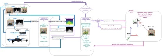
Graphical Abstract

1. Introduction

Multi-rotor aerial vehicles equipped with cameras are capable of covering large areas dynamically, which is why they are valuable for many applications, such as tracking moving objects. When objects in the scene are isolated and distinct from the background, tracking is geneally an achievable task. However, despite decades of research, visual tracking remains a challenging problem in real-world applications due to factors such as partial occlusion, quick and abrupt object motion, lighting changes, and substantial variations in the view point and pose of the target object.
Single-object tracking (SOT) is a fundamental computer vision problem that has several applications, including autonomous vehicles [1,2,3] and surveillance systems [4]. The objective of SOT is to track a defined target within a video sequence using its initial state (position and appearance). SOT approaches [5,6,7,8,9] that utilize the Siamese paradigm are commonly used in 2D and 3D SOT as the Siamese paradigm provides a compromise between performance and speed. Using an appearance-matching strategy, the Siamese model tracks the target in the candidate region using features from the target template and the search area retrieved by a shared backbone.
Since there is no pre-trained object detector involved, single-object trackers are frequently referred to as “generic object trackers” or “model-free trackers” [10,11,12]. From a learning standpoint, model-free visual object tracking is a difficult problem given that there is only one instance of the target in the first frame, and the tracker has to learn the target appearance in the following frames. In our proposed system, we tried to avoid this issue by replacing the template frame with a template set which remains updated based on proposed simple heuristic rules.
The fundamental distinction between detection and tracking is the application of dynamics. During detection, the object is detected independently in each frame. In tracking, we predict the new location of the object in the next frame using estimated dynamics, and then we detect that object. Based on the measurements, we update the estimated dynamics and iterate.
Even while the results of the appearance matching for 3D SOT on the KITTI dataset are decent [13], Zheng et al. [7] noted that KITTI has the following characteristics:
(i)
The subject moves very slightly between two successive frames, preventing a significant change in appearance;
(ii)
There are few or no distractions in the target’s environment.
The aforementioned qualities are not applicable in natural situations. As objects move quickly or the hardware can only handle a limited frame sampling rate, self-occlusion may cause dramatic changes in successive LiDAR views. Additionally, negative samples increase dramatically in scenes where heavy traffic is present. Even humans may find it difficult to identify a target based on its appearance in these situations.
As shown in Figure 1, ourfocus is to track single objects by utilizing only a single RGBD camera rather than the use of other sensors, such as LiDARs, for multiple reasons, such as the use of cameras is cheaper than LiDARs; cameras are lighter in weight than LiDARs, which is very important in the case of multi-rotors; and both sensors cannot see through obstacles, such as heavy rain, snow, and fog.
Based on the above observations, we propose to tackle 3D SOT from a different perspective using the simplicity of a Siamese paradigm [5] with the power of robust monocular depth estimation [14]. The main contributions of the proposed system are as follows:
  • Utilize a monocular-based hybrid-depth estimation technique to overcome the limitations of sensor depth maps.
  • Employ the template set to cover the target object in a variety of poses over time.
  • Introduce the auxiliary object classifier to improve the overall performance of the visual tracker.

2. Related Work

In recent years, visual object tracking has been a prominent research field [15,16]. Due to its necessity and numerous applications, such as autonomous vehicles, robotics, and surveillance, more tracking algorithms are introduced each year [15,16]. Here, we examine the current advancements in the field of visual tracking. To do that, we compare various approaches in terms of the main technique (estimation-based tracking, feature-based tracking, and learning-based tracking); in our comparison, we will consider the advantages, disadvantages, and other details such as the number of tracked objects (single or multiple objects), and whether the tracker works in 2D or 3D space, etc. By the end of this section, we will have outlined a comparison between state-of-the-art deep-learning single-object Trackers.
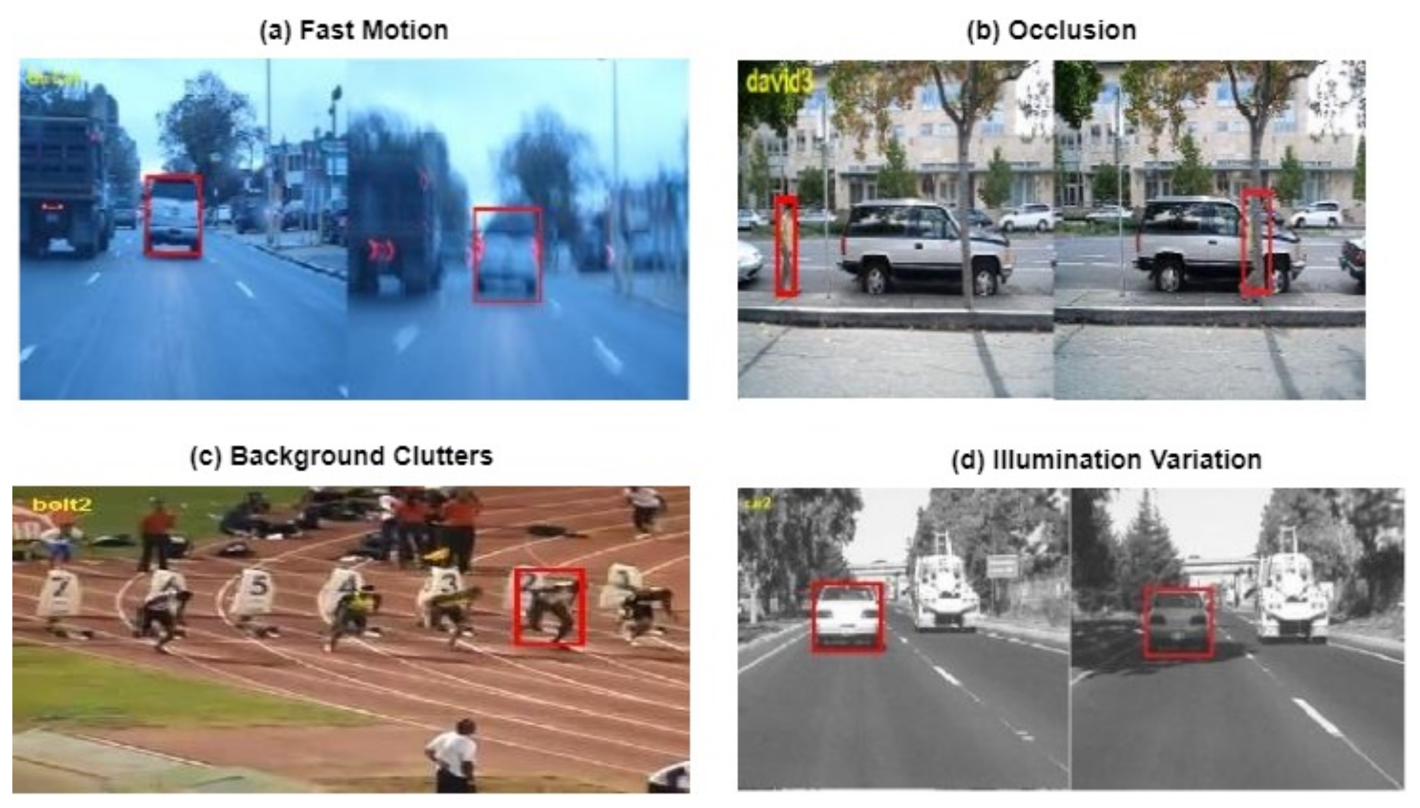
There are many challenges in object tracking [17,18], such as background clutter, scale variation, occlusion, and fast motion, etc. Figure 2 shows some examples from the OTB dataset [18], with each example depicting one of the main challenges. In recent years, many approaches have been proposed to tackle each of the problems; here, we will discuss the state-of-the-art algorithms based on the used tracking techniques.
Estimation-based tracking: To use the Kalman filter [19] in object tracking [20], a dynamic model of the target movement should be designed. A Kalman filter could be used to calculate the position in the case of linear systems with Gaussian errors. For nonlinear dynamic models, other suitable methods are used, such as the extended Kalman filter [21].
Tracking can benefit from the main properties of the Kalman filter [19], which include:
  • Predicting the future location of the object.
  • Forecast correction based on current measurements.
  • Noise reduction caused by incorrect diagnosis.
The vast majority of tracking problems are non-linear. As a result, particle filters have been investigated as a possible solution to such problems. The particle filter is a non-Gaussian-noise measurement model that employs a statistical calculation method known as recursive Monte Carlo. The main concept of the particle filter is to represent the distribution of a set of particles. Each particle is assigned a probability weight, which represents the probability of sampling that particle using the probability density function. One disadvantage of this method is that the particles with the highest probability are selected multiple times, which is overcome by resampling [22].
The JPDA multi-object tracker [23,24,25] is a tracker that can process numerous target detections from multiple sensors. To assign detections to each track, the tracker employs joint probabilistic data association. With a soft assignment, the tracker allows numerous detections to contribute to each track. Tracks are initialized, confirmed, corrected, predicted, and deleted by the tracker. The tracker receives detection reports from the object detector and sensor fusion as inputs. For each track, the state vector and the state estimate-error covariance matrix are estimated by the tracker. Each detection has at least one track associated to it. The tracker creates a new track if the detection cannot be assigned to an existing track.
Feature-based tracking: Using extracted attributes such as texture, color, and optical flow, this category of visual tracker identifies the most similar objects over the upcoming frames. Here, we discuss some of the most important algorithms associated with feature-based trackers. Lucas–Kanade template tracking [26] is one of the first and most popular trackers, originally designed to be able to monitor the optical flow of the image pixels and to determine how they move over time. The problem with this approach was the inaccurate assumption of a constant flow (pure translation) for all pixels in a bigger window for long periods of time. Zhao et al. [27] used local binary patterns (LBP) to describe moving objects and also used a Kalman filter for target tracking. Meanwhile, Zhao et al. [27] inherited the advantages of both LBP and KF, such as the computational simplicity (LBP and KF), the good performance (LBP and KF), the high discriminative power (LBP), and the invariance to the changes in grascale (LBP). On the other hand, this model also inherited the disadvantages of both of them, such as being not invariant to rotations (LBP), and the state variables being normally distributed (KF). Lastly, in terms of time and space, the complexity of computation increases exponentially with the number of neighbors (LBP).
One of the proposed solutions is to compare features (SIFT and HoG) [28,29] instead of pixels, which are hopefully invariant to changes in scale and rotation. Although these algorithms have been used for a long-time, that does not contradict the fact that they have many issues such as highly dimensional feature descriptors (SIFT and HoG), high computation requirements (SIFT and HoG), and low matching accuracy at large angles of rotation and view, which makes them not as reliable as the current deep-learning models.
Learning-based tracking: Discriminative, generative, and reinforcement learning are the three main paradigms used in learning-based tracking. We will review some of the main deep visual object-tracking (VOT) approaches. With the advancement of deep learning, deep features have been used in object trackers. SiamFC [8] was one of the models that used fully convolutional Siamese networks to solve the problem of object tracking. Although SiamFC has many advantages, it has two main disadvantages [30]. First, it only generates the final response scores using the features from the final layer. These high-level features are resistant to noise, but they lack specific target information, making these features insufficient for discrimination when the distractor falls into the same category as the target. Second, the SiamFC training method ensures that each patch in the search region contributes equally to the final response score map. Therefore, regardless of where a distractor appears in the search region, it may produce a high response score and lead the tracking to fail. Later, in SiamRPN [9], the solution was developed using the region proposal network (RPN), which was originally introduced in Faster R-CNN [31] to solve the object detection problem. Therefore, instead of applying a sliding approach on the features, a bunch of proposals are made and then the model both classifies and regresses these proposals using RPN, which has two branches. The first branch is to classify each proposal, whether or not it looks like the template object, and the second branch regresses an offset for the proposed box.DaSiamRPN [6] focused on learning distractor-aware Siamese networks for precise and long-term tracking. To that end, the features of conventional Siamese trackers were initially examined. Zhu et al. [6] recognized that imbalanced training data reduces the separability of the acquired features. To manage this distribution and direct the model’s attention to the semantic distractions, a powerful sampling approach is used during the off-line training phase. Zhu et al. [6] designed a distractor-aware module to perform incremental learning during inference so that the generic embedding can be successfully transferred to the current video domain. Zhu et al. [6] also introduced a straightforward yet efficient local-to-global search region approach for long-term tracking. ATOM (Accurate Tracking by Overlap Maximization) [32] proposed a novel tracking architecture with explicit components for target estimation and classification. The estimation component is trained offline on large-scale datasets to predict the IoU overlap between the target and a bounding-box estimate. The classification component consists of a two-layer fully convolutional network head and is trained online using a dedicated optimization approach. In SiamMask [5], the authors point out that additional information can be encoded in ROW (response of a candidate window) produced by a fully convolutional Siamese network, to generate a pixel-wise binary map. Transformer meets tracker [33]: In contrast to how the transformer is often used in natural language processing applications, Wang et al. [33] redesigned the encoder and decoder of the transformer into two parallel branches within the Siamese-like tracking pipelines. Through attention-based feature reinforcement, the transformer encoder promotes the target templates, which benefits the construction of better tracking models. The object search procedure is made easier by the transformer decoder, which propagates tracking cues from earlier templates to the current frame.
Since our proposed approach is meant to track moving objects in 3D space, we will discuss object localization in 3D space. Indeed, the knowledge of the structure of the 3D environment and the motion of dynamic objects is essential for autonomous navigation [34]. This importance comes from the fact that the 3D structure implicitly depicts the agent’s relative position, and it is also used to help with high-level scene understanding tasks such as detection and segmentation [35]. Recent breakthroughs in deep neural networks (DNNs) have sparked a surge in interest in monocular depth prediction [14,35] and stereo image depth prediction [36], as well as optical flow estimation [37].
Now we will discuss some of the state-of-the-art 3D visual object trackers that operate in three-dimensional space. Eye in the sky [38] is a novel framework for drone-based tracking and 3D object localization systems. It combines CNN-based object detection, multi-object tracking, ground plane estimation, and, finally, 3D localization of the ground targets. In our proposed framework, we use MiDaS [14], besides the depth map generated by the depth sensor, to generate the hybrid-depth map, which is explained in the Section 3. Unlike the relative depth map generated by the MiDaS algorithm [14], the proposed hybrid-depth map estimates the depth measured in meters.
TrackletNet tracker (TNT) [39] is a multi-object tracking method based on a tracklet graph model, incorporating tracklet vertex creation with epipolar geometry and connectivity edge measurement using a multi-scale algorithm, Tracklet-Net.
This description implies several important characteristics of the task at hand:
  • The watermark must include all the required information while remaining placeable and noticeable, even on tiny photos. The created watermark must be compact while still having the ability to hold sufficient information.
  • The watermark must be invisible to the human eye to prevent easy tampering (and, preferably, to basic image parsing tools). If the malefactor is unaware of the existence of the watermark, they may not even attempt to remove or disable it.
Beyond 3D Siamese tracking [7]: The authors of this paper also presented a motion-centric paradigm to handle 3D SOT from a new perspective. They suggested the matching-free two-stage tracker M 2 -Track in line with this concept. At the first stage, M 2 -Track uses motion transformation to localize the target across a series of frames. The target box is then refined at the second stage using motion-assisted shape completion.
While many 3D VOT studies focused on using LiDAR data as the essential data input to their systems [7,38,39,40,41], in our work, we tried to solve the visual object-tracking task using the RGBD data generated by the lightweight and the affordable sensor [42]. To do that, we relied on the SiamMask architecture [5] which originally works in 2D space. We introduced the hybrid-depth maps (explained in detail in the Section 3) to SiamMask to be able to track the objects in 3D environments. In addition, we replaced the template frame used in SiamMask [5] with the template set to give the model the ability to track the moving object from different points of view and without the need to build a 3D model for the moving object. Lastly, we used stereo image triangulation [43] to deproject the position into 3D space, which is followed by a 3D Kalman Filter [19] which helps to remove the measurement noise.
In Table 1, we outlined a comparison between several state-of-the-art deep-learning trackers, along with their tracking framework, published year, dimensional space (2D/3D), backbone network (the feature-extraction network), modules, classification/regression methods (BBR: bounding-box regression. BCE loss: binary cross-entropy loss), training schemes, update schemes (no-update, linear-update, non-linear update), input data format (RGB, LiDAR), tracking speed, re-detection (yes/no, i.e., Y/N).

3. Methodology

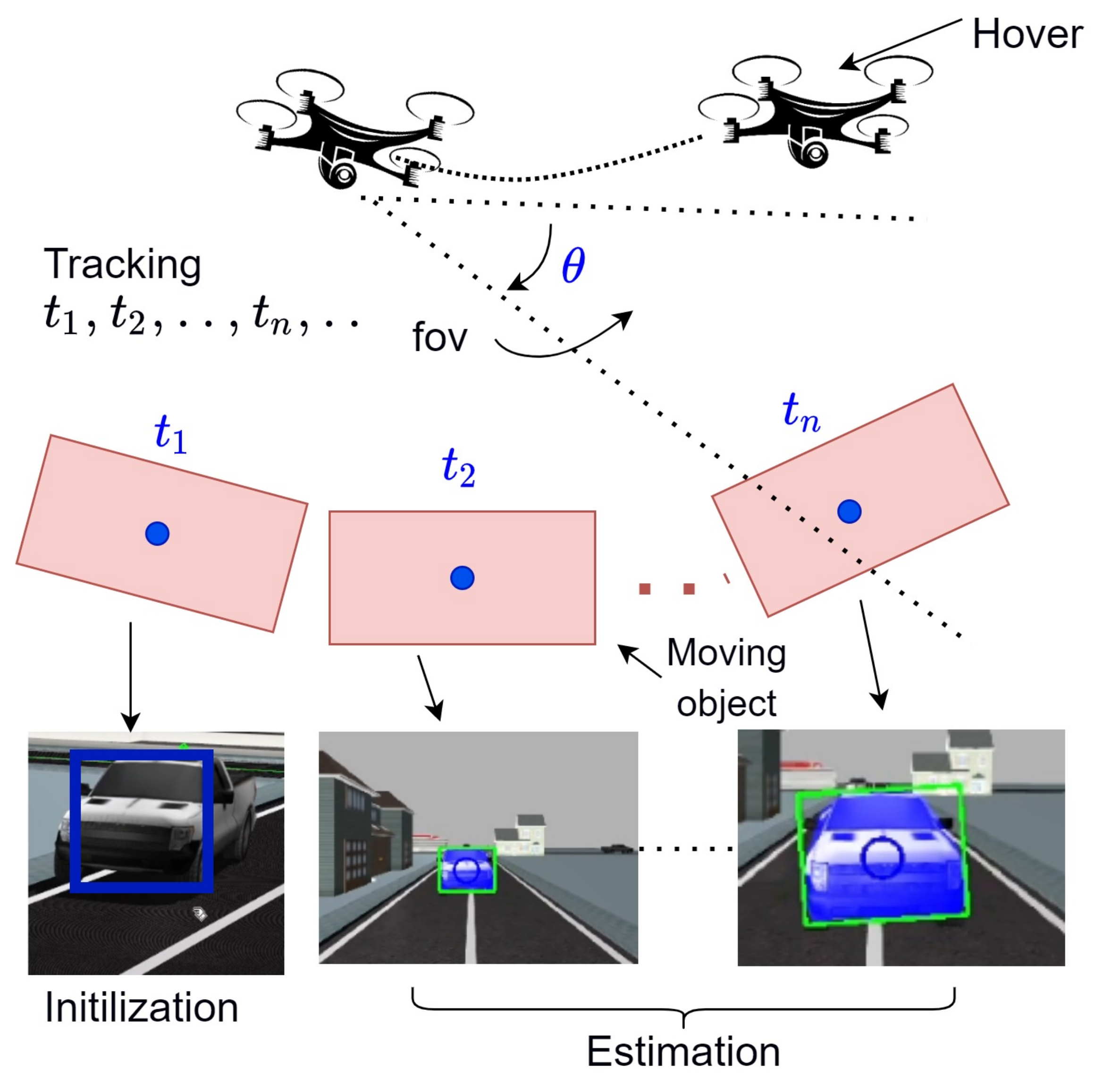
The main goal of this work is to track the moving object from the perspective of the multi-rotor aerial vehicle, Figure 1, where the multi-rotor navigates through the environment while trying to follow the moving object using a real-time visual tracking approach. As shown in Figure 3, the multi-rotor keeps following the moving object until it reaches the location of the moving object and the moving object stops.
There are two sub-tasks in the tracking task: identifying the tracked object and estimating its state. The objective of the tracking mission is to automatically predict the state of the moving object in consecutive frames given its initial state. The proposed framework combines 2D SOT with monocular depth estimation to track moving objects in 3D space. Depth maps are used primarily to maintain awareness of the relevant depth information about target objects.
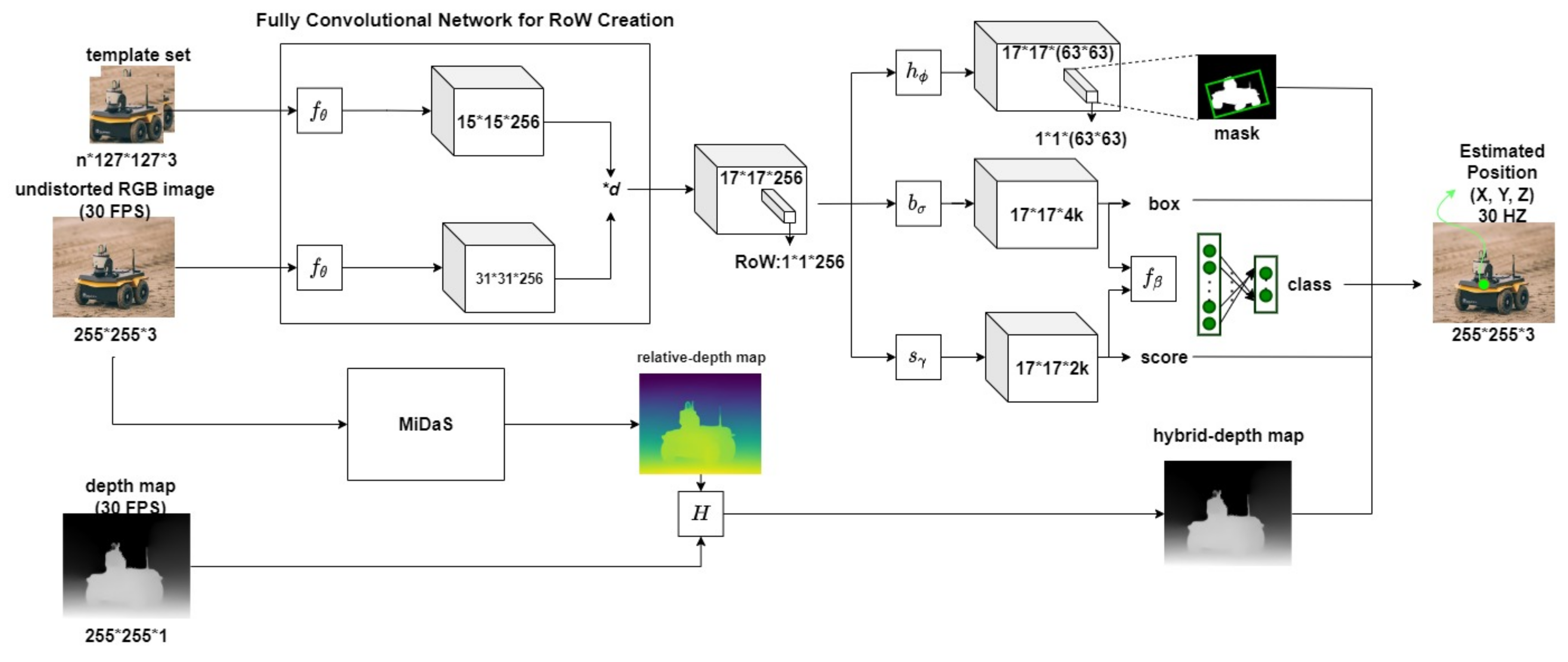
The proposed system basically has a stream of RGB frames and the depth-map inputs (Figure 4). The target object is tracked by the Siamese network which produces a mask, a bounding box, an object class (optional), and an RPN score [31] for the object. In order to estimate the corresponding point in 3D space, a relative depth map [14] is aligned with the depth map [42] to generate the hyprid-depth map. As a result of our experiments, the proposed hyprid-depth map was able to estimate the distance from objects at a distance of more than 20 m, which is four times the range of the currently used depth sensor, which can only estimate the distance from objects at a distance of 5 m [42].
Loss function. To train the classifier f β , we used binary cross entropy as the loss function (1) and Adam as the optimizer.
L c l s = y · log y ^ + ( 1 y ) · log ( 1 y ^ )
where y ^ is the scalar value in the model output, and y is the corresponding target value (0 or 1).
In our experiments, we augmented the architectures of SiamMask [5] and MiDaS [14], where each of them were trained separately:
L 4 B = λ 1 · L mask + λ 2 · L score + λ 3 · L box + λ 4 · L c l s
We refer the reader to [5,8,9] for L mask , L score , and  L box . We have not performed hyperparameter optimization for Equation (2) but we merely set λ 1 = 32 , λ 2 = λ 3 = 1 , like in [5], and λ 4 = 1 .
For MiDaS, we refer to [14]; the used loss function is called the scale- and shift-invariant loss where the loss for a single sample is represented as
L s s i d ^ , d ^ * = 1 2 M i = 1 M ρ d ^ i d ^ i * ,
where d ^ and d ^ * are scaled and shifted versions of the predictions and ground truth, and  ρ defines the specific type of loss function.
Before estimating the position of the target object, we need to estimate the depth of the target object by using the hybrid-depth map H . At each time step, H is calculated as follows
H = η · r · ( NIRD M ^ M ) + D
where H is the hybrid-depth map which conveys the depth estimates in meters, η is a scaling factor, D is the depth map generated by the sensor, and depth ratio r can be evaluated using following expression
r = D NIRD + ϵ
where ϵ is a small fraction to avoid division by zero, and NIRD is the normalized inverted relative depth map, which can be evaluated as
NIRD = R R μ R σ
To evaluate it, we normalize the inverted relative-depth map R by subtracting the mean R μ , then divide by the standard deviation R σ . Therefore,      
R = 1 R
Here, M ^ M is the output of applying the XOR operation (denoted by ⊕) on the binary mask M with 1
M ^ M = M 1
M is the mask for depth points that have values bigger than a small fraction γ , i.e.,
M = D > γ
Despite the fact that many tracking algorithms have been proposed for various tasks and object tracking has been studied for many years, it is still a challenging problem. There is no single tracking algorithm that can be used to accomplish all tasks and in different scenarios. In the case of SiamMask [9], the tracker showed that sometimes it can be distracted from the target object by other distractors or by similar objects in the scene. Working on solving such critical issues could help make multi-rotor-based tracking applications much safer and more reliable. For that purpose, we proposed an auxiliary object classifier and a mechanism for initiating and updating the template set. This mechanism is designed to cover the target object from different points of view from different distances.
At each time step, the proposed framework has two main inputs (the undistorted RGB and depth frames) and estimates the position of the moving object. At the initial step ( j = 0 ), the InitTracker initializes the tracker after adding the cropped template of the target object to the template set. The template set has a maximum size (l) and new candidates will be replace old templates over time. All the templates in the template set could be replaced except for the original template inserted at ( j = 0 ).
The proposed framework components are realised within Algorithm 1.
Algorithm 1 Object visual tracker
Input: Undistorted RGB & depth frames
1:
S 0 InitTracker( RGB 0 , D 0 )
2:
repeat
3:
     RD i + 1 EstimateRelativeDepthMap( RGB i + 1 )
4:
     HD i + 1 GenerateHybridDepthMap( D i + 1 , RD i + 1 )
5:
     S i + 1 EstimateObjectState( S i )
6:
    if StateIsValid( S i + 1 )
7:
         < x i + 1 , y i + 1 , z i + 1 > ApplyProjectionAndKF( HD i + 1 , S i + 1 )
8:
    else
9:
         S i + 1 S i
10:
         < x i + 1 , y i + 1 , z i + 1 > < x i , y i , z i >
11:
    end if
12:
until end of sequence
Let us consider all the steps of Algorithm 1 in detail:
  • EstimateRelativeDepthMap has the RGB image as an input to estimate the relative depth map using the robust monocular depth estimation network [14]; the predicted relative-depth map with the depth map produced by the sensor [42] will be the inputs for the next step.
  • GerenateHybridDepthMap by applying Equation (4). To estimate the hybrid-depth map that has the depth information of the moving object in meters. The process of generating the hybrid-depth map is divided into 3 main steps, as follows
    (i)
    Preprocess the depth map by replacing all non-numeric values with zeros. The result is a 2D array D with values measured in meters.
    (ii)
    Generate from the relative depth map R a 2D array with values [ 0 , 1 ] .
    (iii)
    Apply Equation (4).
  • EstimatingObjectState takes the state vector of the moving object S i as the input and returns the updated state as the output S i + 1 . S i has the details of the target object such as the hybrid-depth maps and the RGB frames of the current and previous time steps [ HD i , HD i + 1 , RGB i , RGB i + 1 ] . The position will be defined in 2D space as the center of the object ( x , y ) . The depth is d = HD [ x , y ] .
    To update the template set there are conditions the candidate template needs to meet. These conditions are as follows
    • Class-specific tracker: the object should be classified by the auxiliary classifier as the desired class.
    • Both trackers: if the detected object satisfies the inequalities (3) below, then the candidate template will be inserted to the template set at j = 1 after the original template frame and before the other templates in the template set:
      | A m a s k i + 1 A m a s k i | < ϵ 1 | A b o x i + 1 A b o x i | < ϵ 2
      where A m a s k and A b o x are the area for the generated mask and the bounding box, respectively. ϵ 1 and ϵ 2 are small fractions.
    Therefore, if the candidate template violates any of the corresponding conditions, the new candidate template will not be inserted to the template set. Before we explain how the template set is used, we need to know that the original template frame has index j = 0 at every time step. The usage of the template set is as follows
    (i)
    Use the original template frame.
    (ii)
    The conditions (3) above must be satisfied and the objectness probability (RPN score) should be greater than a threshold α . Other than that, the template frame is skipped to the next most recent frame in the template set.
    (iii)
    Repeat (ii) if needed for n times (in our experiments n = 2 ).
    (iv)
    Return the estimated object state.
  • ApplyProjectionAndKF: A 3D Kalman filter [19] will remove measurement noise after a stereo image triangulation [43] deprojects the position into 3D space.
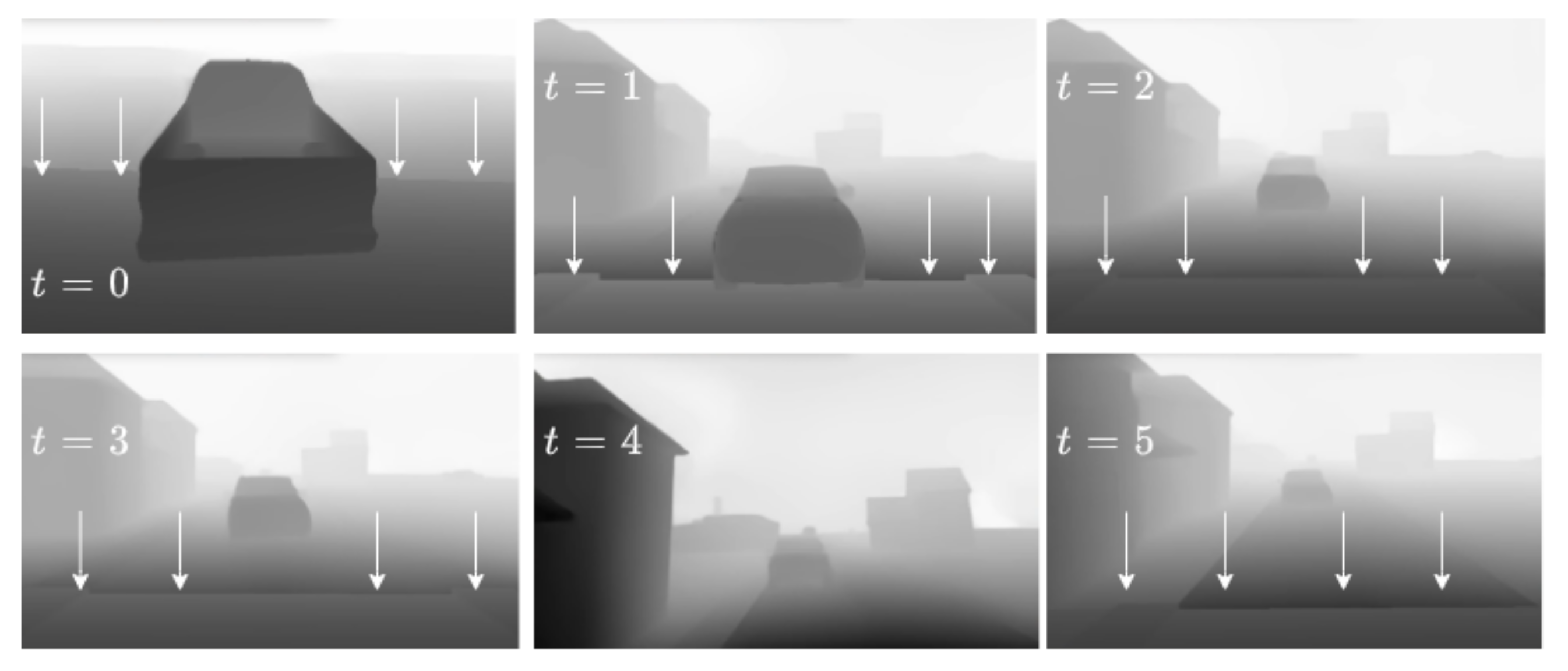
As shown in Figure 4, the hybrid-depth map is generated from both the MiDaS relative-depth map [14] and the Intel RealSense depth map [42]. The alignment of these two maps was explained in detail in Algorithm 1. Figure 5 shows the generated hyprid-depth map using the proposed approach.
Similarly to SiamMask [5], ResNet50 [49] is used until the final convolutional layer of the 4th stage as the backbone f θ for both Siamese Network [5] branches. The main goal of h ϕ is to predict w × h binary masks (one for each RoW). Basically, h ϕ is a simple two-layer network with learnable parameters ϕ .
In the proposed system, a ResNet18 [49] was used to classify the object detected by the SiamRPN branches [9], to stabilize tracking and make the model less prone to distractors. We have two different settings to run in the proposed system:
  • Generic moving-object tracker: in this case, the object will be classified using the Siamese tracker with the help of the frames in the template set.
  • Class-specific moving-object tracker: in this case, the tracker will have an auxiliary object classifier which makes sure to avoid distractors and the possible foreground/background confusions by the RPN network.
The experiment was performed by training ResNet18 with a binary classification layer. Two datasets were utilized to train the binary classifier. The moving object class is represented by the Stanford Cars dataset (16,185 photos of 196 car classes) [50]. In contrast, the Describable Textures Dataset (DTD) [51] was applied to the non-moving object class. The DTD dataset contains 5640 photos sorted into 47 categories influenced by human sight.

4. Results

The trackers were tested in two simulation environments, Figure 6, to assess the performance in different cases. The GitHub repository includes a video with the experiment results. For visual tracker evaluation, the VOT (visual object tracking) benchmarks were used [52,53,54]; all of the benchmark datasets are annotated with rotated bounding boxes. The comparison over the three benchmarks was performed using the official VOT toolkit and the expected average overlap (EAO) [55] (EAO is a metric which takes into consideration the accuracy and the robustness of the visual tracker).
The tracker was tested in the simulation environment utilizing the Iris drone with the Intel Realsense Depth Camera [42]. The tracker was implemented using Python 3.6 and ROS1. We used a computer with a 2.6 GHz CPU, an NVIDIA GeForce RTX 2060 6 GB GPU, and 16 GB of RAM for the simulated environment. The simulated experiments were performed in a Gazebo software. The local planner [56] was used to generate the optimal control to maneuver the quad-rotor considering close-in obstacles and system dynamics. Code and results are available at: https://github.com/mhd-medfa/Single-Object-Tracker.

4.1. Experiment 1: Generic and Class-Specific Trackers

Firstly, this experiment was carried out in the basic simulation environment, Figure 6. We should mention here that the proposed framework has two tracking approaches:
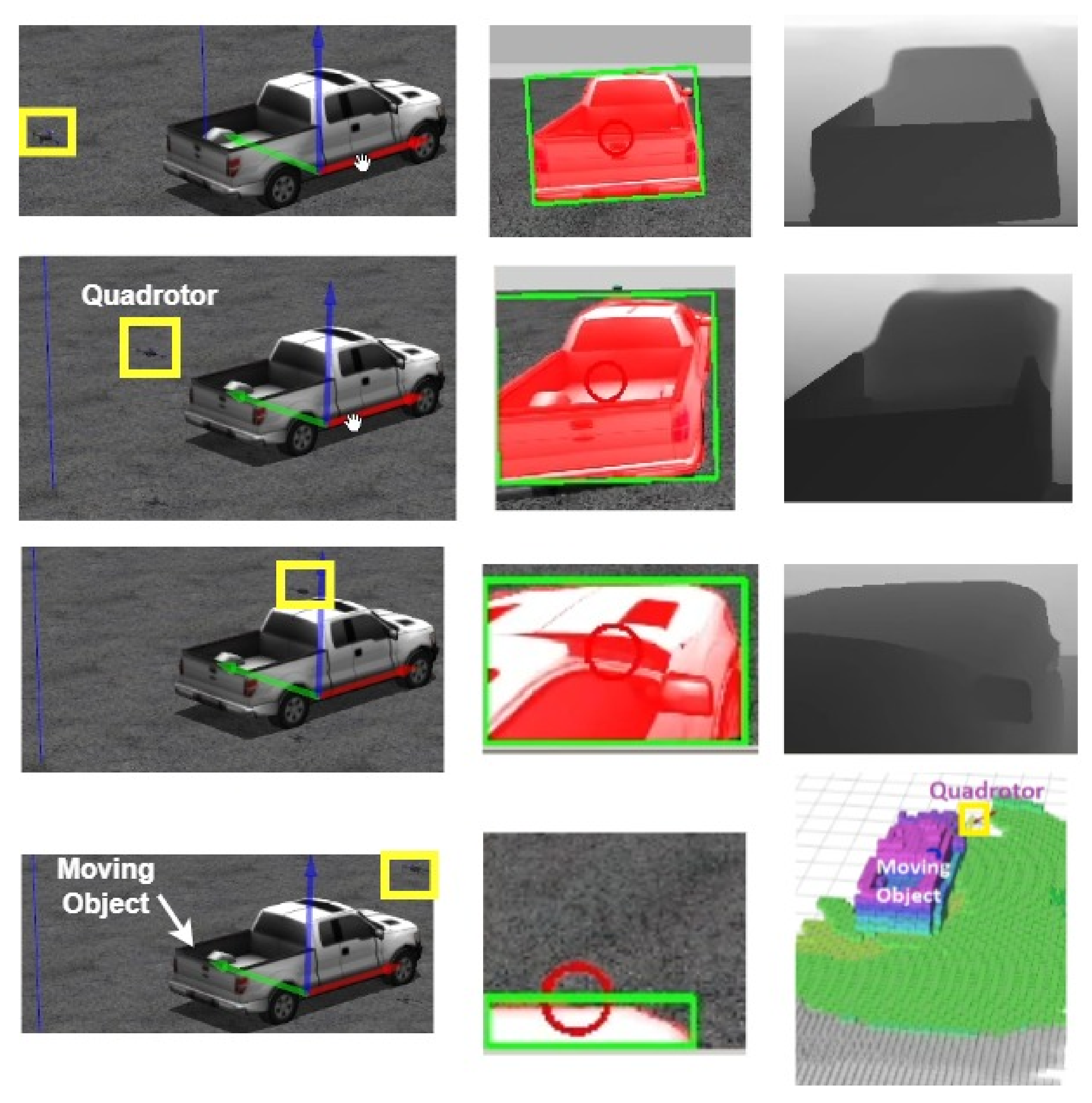
  • Generic tracker. Figure 7 shows how the tracker, using the Siamese tracker with the help of the template set and the hybrid depth map, was able to track the target object. The experiment showed that the tracker passed the moving object.
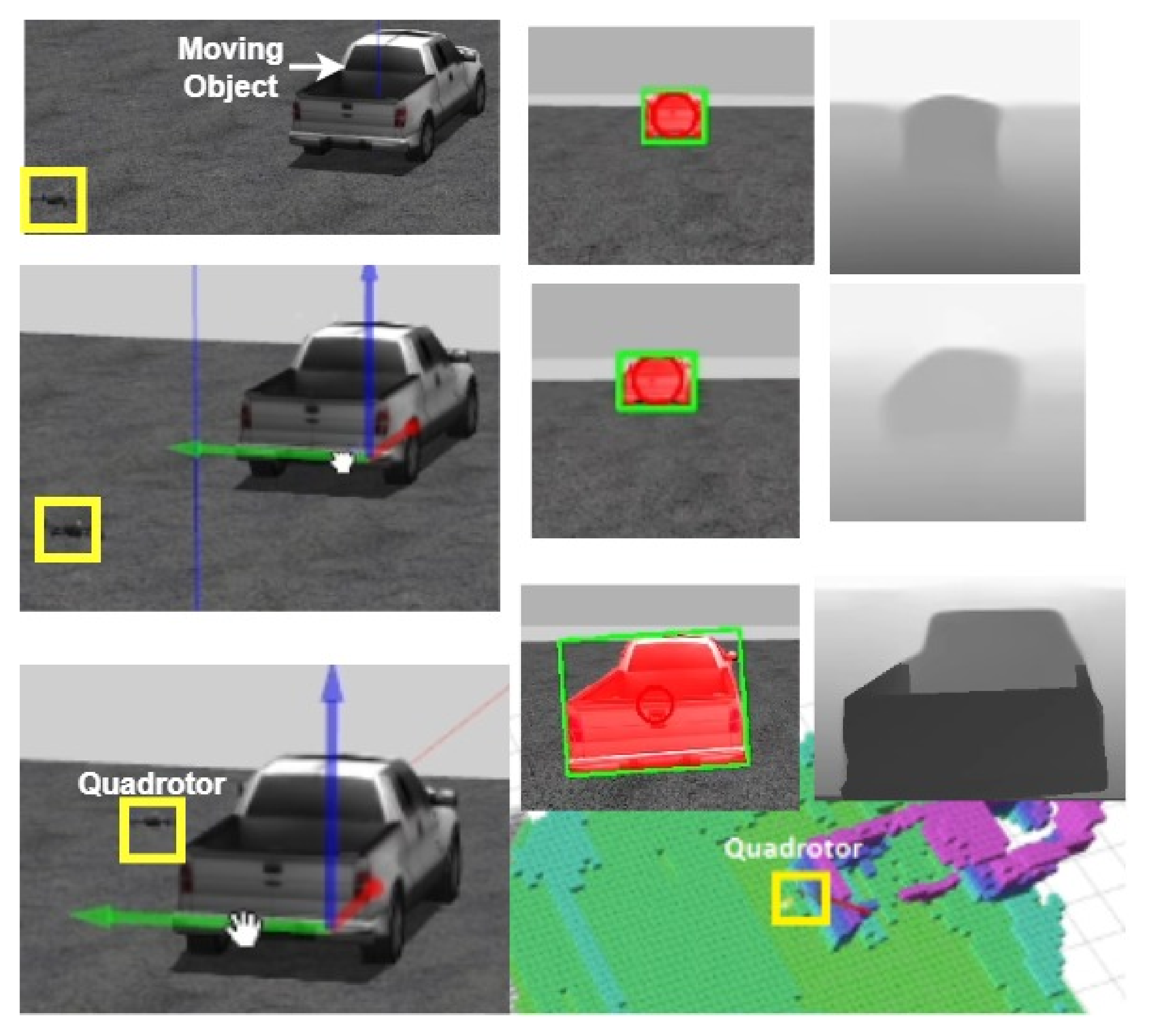
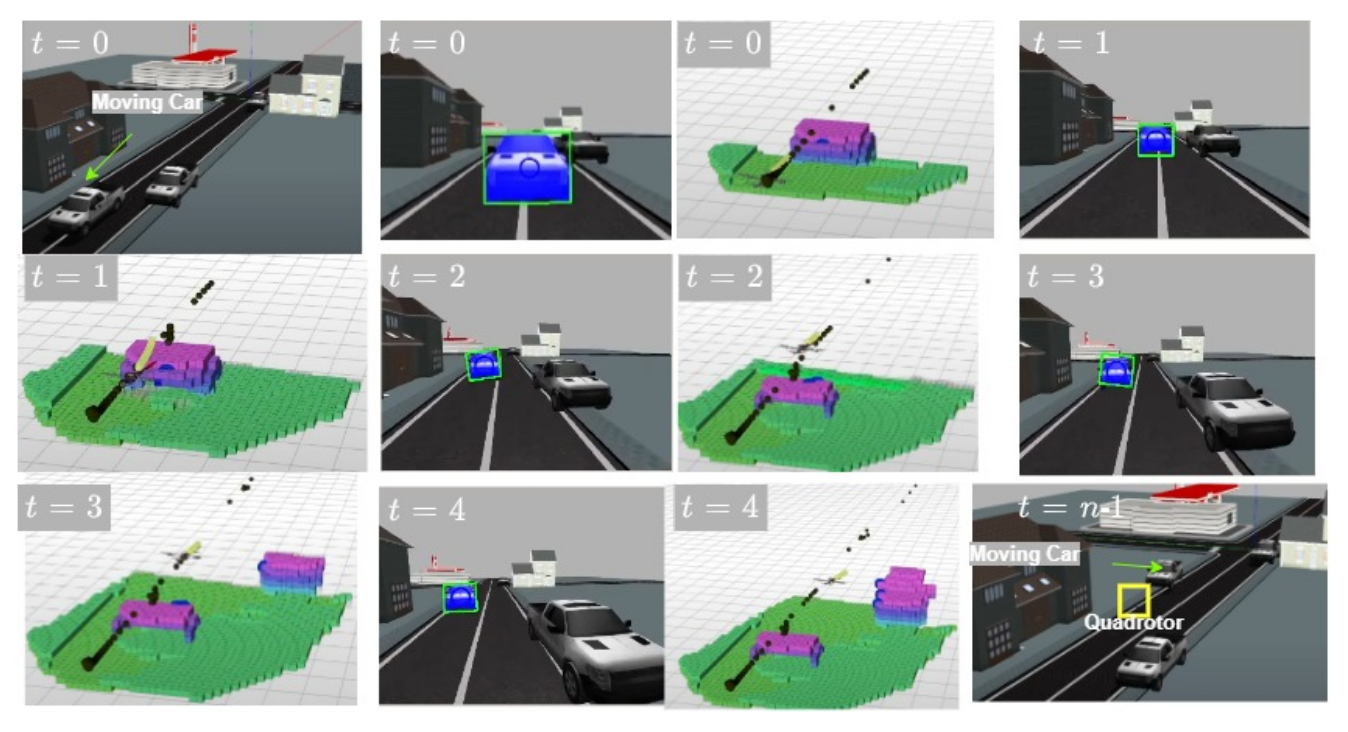
  • Class-specific tracker. Figure 8 shows that by involving the auxiliary object classifier, the object tracker did not pass the moving object. The responsibility of this classifier is to stabilize the tracking process.
A primary drawback of the generic tracker is that the multi-rotor may pass the target object due to the fact that the Siamese tracker measures the similarity between the template frame and input frame, which makes the tracker detect the object even if only small part of the object is showing in the scene [5].This issue is handled in the class-specific mode, in which the object classifier classifies the RPN-proposed item at each time step, so that if the target object is closer than d[meters] or if the tracker could not recognize the target object (i.e., the auxiliary classifier classified the detected object into a different class of objects), then the multi-rotor will keep hovering at the same position until the conditions change (i.e., the moving object becomes farther than d[meters]). All that helps keep the target object in the scene without passing the tracked object, as shown in Figure 8.

4.2. Experiment 2: Different Case Scenarios

In this experiment, we try to record the behavior of the tracking system in the following scenarios:

4.2.1. The Basic Moving-Object Tracking

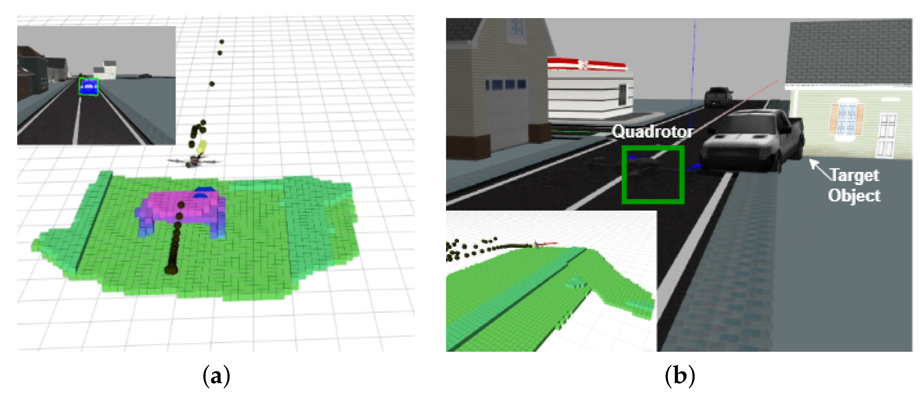
In this case of Figure 9, the multi-rotor followed the moving object. The moving car has no other semantically similar objects in the scene. In the experiment, the car was not very fast, so the multi-rotor kept pace with the moving car. At the beginning, the visual tracker was running without running the planner [56]. When the moving object became far from the multi-rotor (about 10 m away), the multi-rotor tracked the moving object. The multi-rotor stopped when the distance from the moving object became less than the predefined threshold α = 5 [m]. When the object was far from the multi-rotor, the estimated depth of the moving object was not accurate, but the multi-rotor still managed to track it. As the multi-rotor approached the moving object, depth estimation became more accurate. For more details, check the video attached in the GitHub repository.

4.2.2. Tracking One of Multiple Identical Objects

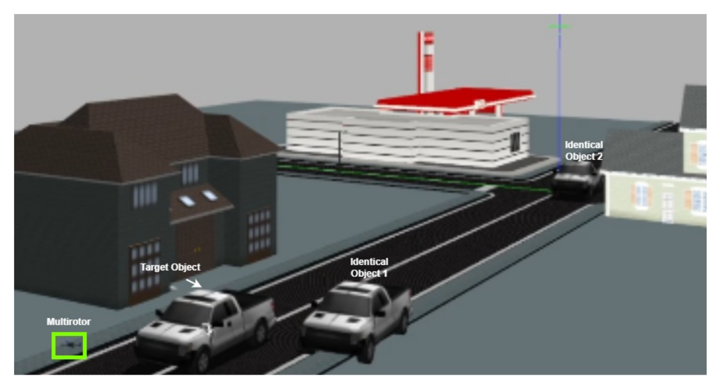
As shown in Figure 10, the experiment had three identical objects while the goal was tracking one of these objects. Figure 11 shows how the proposed managed to track the car (moving object) with no conflict with the other similar objects.

4.2.3. Tracking a Far Moving Object

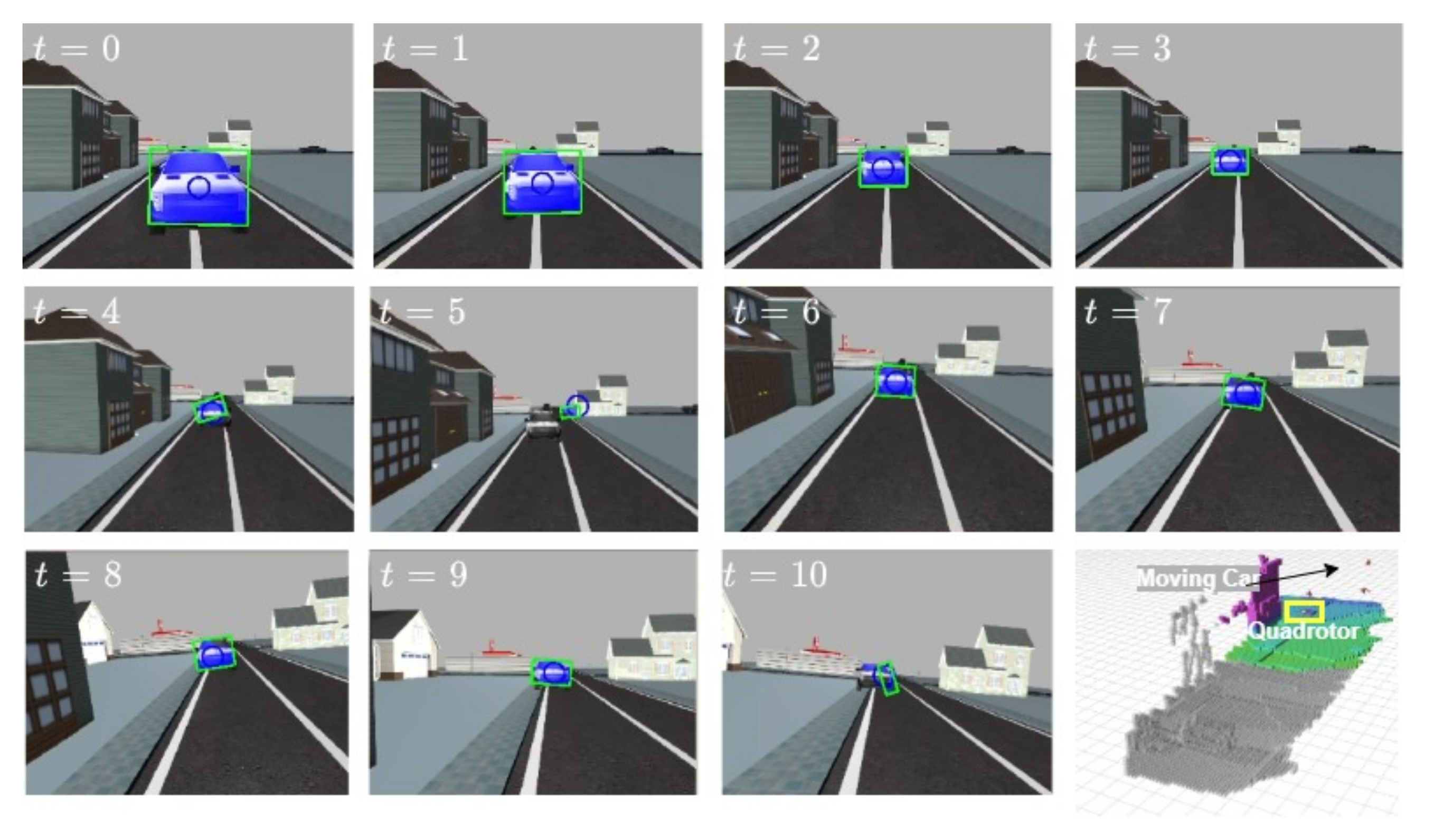
The experiment shows how the tracking system will behave in the case of tracking a far moving object (Figure 12). The result shows that the visual object tracker managed to track the far moving objects even when the object was far from the multi-rotor. The experiment is shown in the results video in the GitHub repository.

4.3. Depth-Estimation Analysis

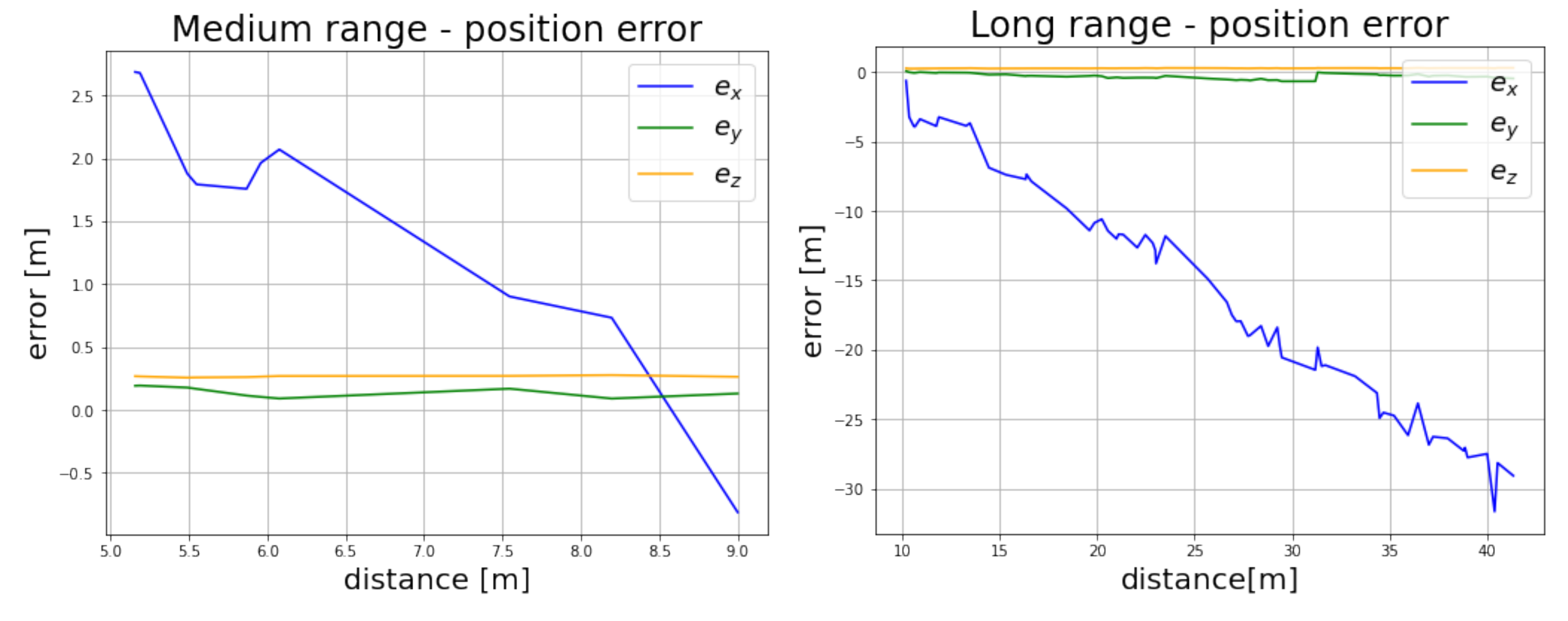
For depth estimation, the intended experiment had the target object moving over almost a straight line so we could observe the depth-estimation accuracy and that explains the relatively small errors on the y and z axes in the medium-range experiment, Table 2, as an example. The experiments are classified into three categories based on the distance between the object and the camera frame and considering a ToF (time-of-flight) camera [57] was used:
  • Short (typical) range (5 m or less)
  • Medium range (between 5 and 10 m)
  • Long range (more than 10 m)
Table 2. Medium-range performance.
x [m]y [m]z [m]Position [m]
RMSE1.11560.16180.26281.1576
MSE1.03140.15660.26251.34
MAE1.2450.02620.06911.4506
The experiments were conducted in an open-source [58] customized simulation environment, Figure 6.

4.3.1. Short (Typical) Range

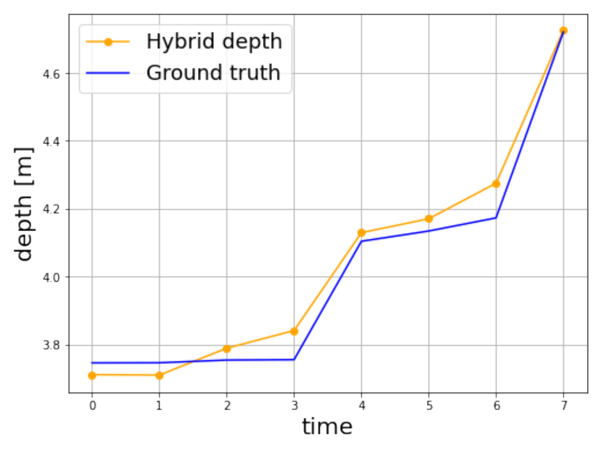
In the typical range, Figure 13, the hybrid-depth estimation matches the sensor depth estimation, and the reason is that in short ranges, our proposed framework relies on the data measured by the sensor. While the claimed max. range of the sensor is up to 6 m [42], in our experiments the sensor depth measurements was available only up to the range of 5 m.

4.3.2. Medium Range

Medium range shows the interesting part of the hybrid-depth approach. The estimation of depth is in the range of 5 to 10 m.
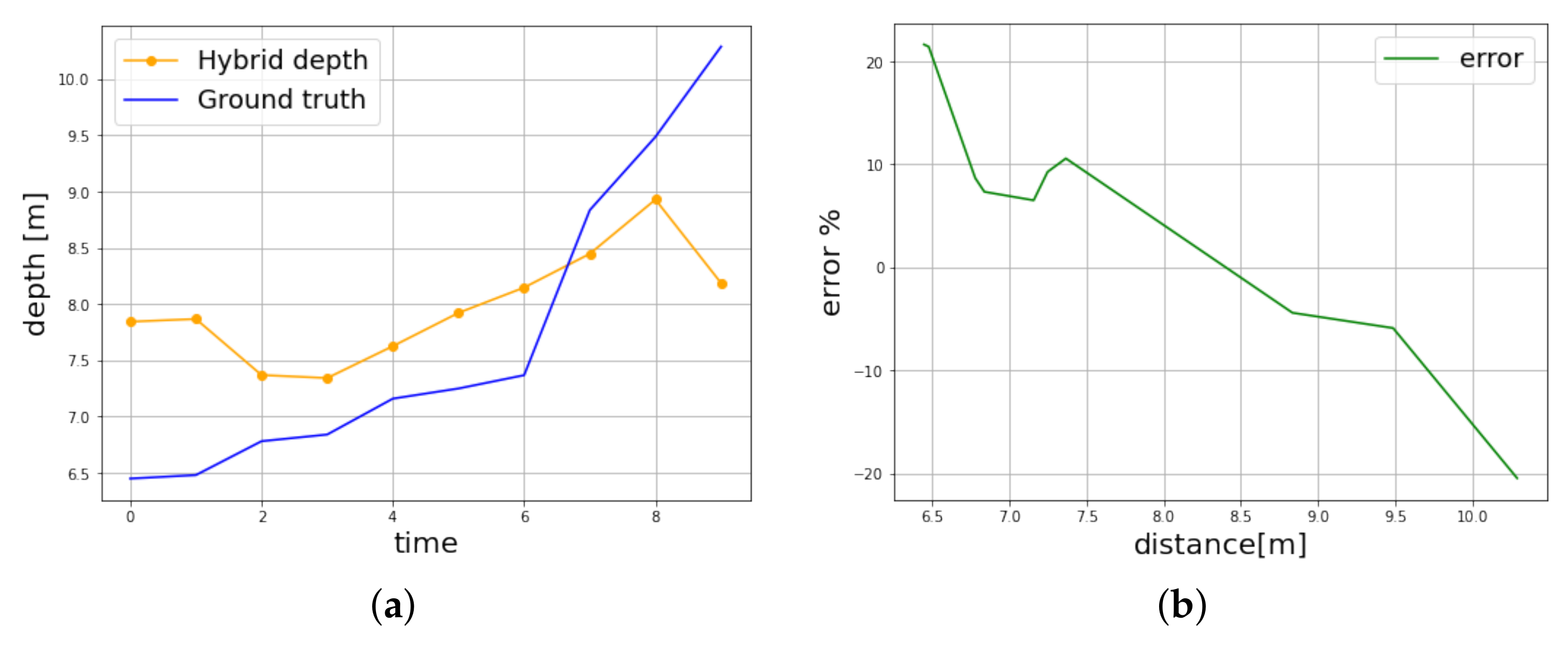
As shown in Figure 14, the experimental results show that the maximum abstract depth error is around 20 % . The root-mean-square deviation (error) RMSD or RMSE can be computed as
RMSE = i = 1 N x i x ^ i 2 N
where N: is the number of depth samples, x i : is the ground truth at point i, and x ^ i is the estimated depth at point i. The mean-square-error MSE is evaluated as follows
MSE = i = 1 N x i x ^ i 2 N
where N: is the number of depth samples, x i : is the ground truth at point i, and x ^ i is the estimated depth at point i. In addition, the mean absolute error MAE was computed using following expression
MAE = i = 1 n x i x ^ i N
where N: is the number of depth samples, x i is the ground truth at point i, and x ^ i is the estimated depth at point i.
To identify how far the predictions fall from the ground truth, RMSE Equation (10), MSE Equation (11) and MAE Equation (12) were measured on random samples collected in the medium range (Table 2). The goal of the experiment is to observe the accuracy of depth estimation by moving the target object along a straight line. This explains the relatively small errors on the y and z axes.

4.3.3. Long Range

Depth estimation performed poorly in long ranges, and the estimated depth values oscillate between 9 and 12 m with a linearly growing error over distance. However, current performance will be enough in the case of a quadrotor with a similar or higher range of speed than the moving object (Figure 15 and Figure 16).

4.4. Visual Object-Tracker Evaluation

In this subsection, we explore the general performance regarding speed and the performance on the established visual-tracking benchmarks VOT-2016 [52],VOT-2018 [53], and VOT-2019 [54]. On the used VOT benchmarks, the performance is measured in terms of accuracy, robustness, and expected average overlap (EAO), as shown in Table 3 and Table 4, where EAO is used to rank trackers. Additionally, as shown in Table 5, we considered the speed in the comparison on the VOT-2018 dataset.
To run our experiments, we had access to a server with a single Nvidia Quadro P4000 GPU with Ubuntu 18.04. The comparison with other nine state-of-the-art single-object trackers (Table 5), showed that the proposed tracker performed better in terms of accuracy on the VOT-2018 dataset. While in Table 3, the generic tracker had a better robustness score than the SiamMask model [5].

5. Conclusions

A fundamental computer vision problem known as single-object tracking (SOT) has numerous applications, including surveillance systems [4], autonomous vehicles [1,2] and aerial photography [61]. Its objective is to track a particular target within a video series using only its initial state (appearance and location).
In this paper, we proposed a framework which allows multi-rotor aerial vehicles to track moving objects in real time. We suggested having a set of templates, so that we could cover the object from various perspectives throughout time. We developed a method to overcome the limitations of popular commercial depth sensors by combining their data with relative depth maps produced by a machine-learning model for depth estimation [14] to create a hybrid-depth map. Lastly, an object classifier was utilized to overcome the inherited behaviour of the Siamese visual tracker and to limit the effect of distractors and false-positive detected objects.
Apart from the numerous advantages for the proposed framework, there are some limitations to take into consideration, such as the fact that the proposed hybrid-depth estimation approach showed some weaknesses in long-range distances. However, in the case of the moving-object tracking problem, this limitation could not be considered to be a critical issue because the distance estimation will become more and more accurate as the multi-rotor aerial vehicle reaches the target object.
In future work, the main focus will be to build multi-class non-contrastive incremental learning for the following reasons:
  • Non-contrastive learning will be used for the opportunity of having a better representation [62] which could tackle problems such as occlusion, illumination variation, etc.
  • Self-supervised incremental learning will be used to create a more effective tracking framework which could be trained on the new classes without suffering from the forgetting problem [63].

Author Contributions

Conceptualization, G.K.; Data curation, M.A.M.; Formal analysis, G.K.; Investigation, G.K.; Methodology, M.A.M.; Resources, A.K.; Software, M.A.M.; Supervision, A.K.; Validation, M.A.M.; Visualization, M.A.M.; Writing–review & editing, A.K. All authors have read and agreed to the published version of the manuscript.

Funding

This research received no external funding.

Data Availability Statement

Code and results are available at: https://github.com/mhd-medfa/Single-Object-Tracker.

Conflicts of Interest

The authors declare no conflict of interest.

References

  1. Qi, C.R.; Zhou, Y.; Najibi, M.; Sun, P.; Vo, K.; Deng, B.; Anguelov, D. Offboard 3d object detection from point cloud sequences. In Proceedings of the IEEE/CVF Conference on Computer Vision and Pattern Recognition, Nashville, TN, USA, 20–25 June 2021; pp. 6134–6144. [Google Scholar]
  2. Yan, X.; Zheng, C.; Li, Z.; Wang, S.; Cui, S. Pointasnl: Robust point clouds processing using nonlocal neural networks with adaptive sampling. In Proceedings of the IEEE/CVF Conference on Computer Vision and Pattern Recognition, Seattle, WA, USA, 13–19 June 2020; pp. 5589–5598. [Google Scholar]
  3. Yan, X.; Gao, J.; Li, J.; Zhang, R.; Li, Z.; Huang, R.; Cui, S. Sparse single sweep lidar point cloud segmentation via learning contextual shape priors from scene completion. In Proceedings of the AAAI Conference on Artificial Intelligence, Vancouver, BC, Canada, 2–9 February 2021; Volume 35, pp. 3101–3109. [Google Scholar]
  4. Thys, S.; Van Ranst, W.; Goedemé, T. Fooling automated surveillance cameras: Adversarial patches to attack person detection. In Proceedings of the IEEE/CVF Conference on Computer Vision and Pattern Recognition Workshops, Long Beach, CA, USA, 16–20 June 2019. [Google Scholar]
  5. Wang, Q.; Zhang, L.; Bertinetto, L.; Hu, W.; Torr, P.H. Fast online object tracking and segmentation: A unifying approach. In Proceedings of the IEEE/CVF Conference on Computer Vision and Pattern Recognition, Long Beach, CA, USA, 16–20 June 2019; pp. 1328–1338. [Google Scholar]
  6. Zhu, Z.; Wang, Q.; Li, B.; Wu, W.; Yan, J.; Hu, W. Distractor-aware siamese networks for visual object tracking. In Proceedings of the European Conference on Computer Vision (ECCV), Munich, Germany, 8–14 September 2018; pp. 101–117. [Google Scholar]
  7. Zheng, C.; Yan, X.; Zhang, H.; Wang, B.; Cheng, S.; Cui, S.; Li, Z. Beyond 3D Siamese Tracking: A Motion-Centric Paradigm for 3D Single Object Tracking in Point Clouds. In Proceedings of the IEEE/CVF Conference on Computer Vision and Pattern Recognition, New Orleans, LA, USA, 19–20 June 2022; pp. 8111–8120. [Google Scholar]
  8. Bertinetto, L.; Valmadre, J.; Henriques, J.F.; Vedaldi, A.; Torr, P.H. Fully-convolutional siamese networks for object tracking. In Proceedings of the European Conference on Computer Vision, Amsterdam, The Netherlands, 11–14 October 2016; Springer: Berlin/Heidelberg, Germany, 2016; pp. 850–865. [Google Scholar]
  9. Li, B.; Yan, J.; Wu, W.; Zhu, Z.; Hu, X. High performance visual tracking with siamese region proposal network. In Proceedings of the IEEE conference on Computer Vision and Pattern Recognition, Salt Lake City, UT, USA, 18–22 June 2018; pp. 8971–8980. [Google Scholar]
  10. Zhang, T.; Liu, S.; Xu, C.; Yan, S.; Ghanem, B.; Ahuja, N.; Yang, M.H. Structural sparse tracking. In Proceedings of the IEEE conference on computer vision and pattern recognition, Boston, MA, USA, 7–12 June 2015; pp. 150–158. [Google Scholar]
  11. Collins, R.T.; Liu, Y.; Leordeanu, M. Online selection of discriminative tracking features. IEEE Trans. Pattern Anal. Mach. Intell. 2005, 27, 1631–1643. [Google Scholar] [CrossRef] [PubMed]
  12. Ross, D.A.; Lim, J.; Lin, R.S.; Yang, M.H. Incremental learning for robust visual tracking. Int. J. Comput. Vis. 2008, 77, 125–141. [Google Scholar] [CrossRef]
  13. Geiger, A.; Lenz, P.; Urtasun, R. Are we ready for autonomous driving? The kitti vision benchmark suite. In Proceedings of the 2012 IEEE Conference on Computer Vision and Pattern Recognition, Providence, RI, USA, 16–21 June 2012; pp. 3354–3361. [Google Scholar]
  14. Ranftl, R.; Lasinger, K.; Hafner, D.; Schindler, K.; Koltun, V. Towards robust monocular depth estimation: Mixing datasets for zero-shot cross-dataset transfer. IEEE Trans. Pattern Anal. Mach. Intell. 2020, 44, 1623–1637. [Google Scholar] [CrossRef] [PubMed]
  15. Luo, W.; Xing, J.; Milan, A.; Zhang, X.; Liu, W.; Kim, T.K. Multiple object tracking: A literature review. Artif. Intell. 2021, 293, 103448. [Google Scholar] [CrossRef]
  16. Soleimanitaleb, Z.; Keyvanrad, M.A. Single Object Tracking: A Survey of Methods, Datasets, and Evaluation Metrics. arXiv 2022, arXiv:2201.13066. [Google Scholar]
  17. Wang, Q.; Chen, F.; Xu, W.; Yang, M.H. An experimental comparison of online object-tracking algorithms. Wavelets Sparsity XIV 2011, 8138, 311–321. [Google Scholar]
  18. Wu, Y.; Lim, J.; Yang, M.H. Online object tracking: A benchmark. In Proceedings of the IEEE Conference on Computer Vision and Pattern Recognition, Portland, OR, USA, 23–28 June 2013; pp. 2411–2418. [Google Scholar]
  19. Kalman, R.E. A new approach to linear filtering and prediction problems. J. Basic Eng. 1960, 82, 35–45. [Google Scholar] [CrossRef] [Green Version]
  20. Najafzadeh, N.; Fotouhi, M.; Kasaei, S. Multiple soccer players tracking. In Proceedings of the 2015 The International Symposium on Artificial Intelligence and Signal Processing (AISP), Mashhad, Iran, 3–5 March 2015; pp. 310–315. [Google Scholar]
  21. Julier, S.J.; Uhlmann, J.K. New extension of the Kalman filter to nonlinear systems. In Proceedings of the Signal Processing, Sensor Fusion, and Target Recognition VI, Orlando, FL, USA, 21–25 April 1997; Volume 3068, pp. 182–193. [Google Scholar]
  22. Boers, Y.; Driessen, J.N. Particle filter based detection for tracking. In Proceedings of the 2001 American Control Conference, (Cat. No. 01CH37148), Arlington, VA, USA, 25–27 June 2001; Volume 6, pp. 4393–4397. [Google Scholar]
  23. Fortmann, T.; Bar-Shalom, Y.; Scheffe, M. Sonar tracking of multiple targets using joint probabilistic data association. IEEE J. Ocean. Eng. 1983, 8, 173–184. [Google Scholar] [CrossRef] [Green Version]
  24. Musicki, D.; Evans, R. Joint integrated probabilistic data association: JIPDA. IEEE Trans. Aerosp. Electron. Syst. 2004, 40, 1093–1099. [Google Scholar] [CrossRef]
  25. Svensson, L.; Svensson, D.; Guerriero, M.; Willett, P. Set JPDA Filter for Multitarget Tracking. IEEE Trans. Signal Process. 2011, 59, 4677–4691. [Google Scholar] [CrossRef] [Green Version]
  26. Lucas, B.D.; Kanade, T. An Iterative Image Registration Technique with an Application to Stereo Vision. In Proceedings of the 7th International Joint Conference on Artificial Intelligence (IJCAI ’81), Vancouver, BC, Canada, 24–28 August 1981; Volume 81. [Google Scholar]
  27. Hu, Y.; Zhao, W.; Wang, L. Vision-based target tracking and collision avoidance for two autonomous robotic fish. IEEE Trans. Ind. Electron. 2009, 56, 1401–1410. [Google Scholar]
  28. Lowe, D.G. Distinctive image features from scale-invariant keypoints. Int. J. Comput. Vis. 2004, 60, 91–110. [Google Scholar] [CrossRef]
  29. Dalal, N.; Triggs, B. Histograms of oriented gradients for human detection. In Proceedings of the 2005 IEEE Computer Society Conference on Computer Vision and Pattern Recognition (CVPR’05), San Diego, CA, USA, 20–25 June 2005; Volume 1, pp. 886–893. [Google Scholar]
  30. Li, C.; Xing, Q.; Ma, Z. HKSiamFC: Visual-tracking framework using prior information provided by staple and kalman filter. Sensors 2020, 20, 2137. [Google Scholar] [CrossRef] [PubMed]
  31. Ren, S.; He, K.; Girshick, R.; Sun, J. Faster r-cnn: Towards real-time object detection with region proposal networks. In Proceedings of the 28th International Conference on Neural Information Processing Systems, Montreal, QC, Canada, 7–12 December 2015. [Google Scholar]
  32. Danelljan, M.; Bhat, G.; Khan, F.S.; Felsberg, M. Atom: Accurate tracking by overlap maximization. In Proceedings of the IEEE/CVF Conference on Computer Vision and Pattern Recognition, Long Beach, CA, USA, 16–20 June 2019; pp. 4660–4669. [Google Scholar]
  33. Wang, N.; Zhou, W.; Wang, J.; Li, H. Transformer meets tracker: Exploiting temporal context for robust visual tracking. In Proceedings of the IEEE/CVF Conference on Computer Vision and Pattern Recognition, Nashville, TN, USA, 19–25 June 2021; pp. 1571–1580. [Google Scholar]
  34. Geiger, A.; Lauer, M.; Wojek, C.; Stiller, C.; Urtasun, R. 3d traffic scene understanding from movable platforms. IEEE Trans. Pattern Anal. Mach. Intell. 2013, 36, 1012–1025. [Google Scholar] [CrossRef] [PubMed] [Green Version]
  35. Lee, S.; Im, S.; Lin, S.; Kweon, I.S. Learning monocular depth in dynamic scenes via instance-aware projection consistency. In Proceedings of the AAAI Conference on Artificial Intelligence, Vancouver, BC, Canada, 2–9 February 2021; Volume 35, pp. 1863–1872. [Google Scholar]
  36. Chang, J.R.; Chen, Y.S. Pyramid stereo matching network. In Proceedings of the IEEE Conference on Computer Vision and Pattern Recognition, Salt Lake City, UT, USA, 18–22 June 2018; pp. 5410–5418. [Google Scholar]
  37. Sun, D.; Yang, X.; Liu, M.Y.; Kautz, J. Pwc-net: Cnns for optical flow using pyramid, warping, and cost volume. In Proceedings of the IEEE Conference on Computer Vision and Pattern Recognition, Salt Lake City, UT, USA, 18–22 June 2018; pp. 8934–8943. [Google Scholar]
  38. Zhang, H.; Wang, G.; Lei, Z.; Hwang, J.N. Eye in the sky: Drone-based object tracking and 3d localization. In Proceedings of the 27th ACM International Conference on Multimedia, Nice, France, 21–25 October 2019; pp. 899–907. [Google Scholar]
  39. Wang, G.; Wang, Y.; Zhang, H.; Gu, R.; Hwang, J.N. Exploit the connectivity: Multi-object tracking with trackletnet. In Proceedings of the 27th ACM International Conference on Multimedia, Nice, France, 21–25 October 2019; pp. 482–490. [Google Scholar]
  40. Fang, Z.; Zhou, S.; Cui, Y.; Scherer, S. 3d-siamrpn: An end-to-end learning method for real-time 3d single object tracking using raw point cloud. IEEE Sens. J. 2020, 21, 4995–5011. [Google Scholar] [CrossRef]
  41. Qi, H.; Feng, C.; Cao, Z.; Zhao, F.; Xiao, Y. P2b: Point-to-box network for 3d object tracking in point clouds. In Proceedings of the IEEE/CVF Conference on Computer Vision and Pattern Recognition, Seattle, WA, USA, 14–19 June 2020; pp. 6329–6338. [Google Scholar]
  42. Keselman, L.; Iselin Woodfill, J.; Grunnet-Jepsen, A.; Bhowmik, A. Intel realsense stereoscopic depth cameras. In Proceedings of the IEEE Conference on Computer Vision and Pattern Recognition Workshops, Honolulu, HI, USA, 21–26 July 2017; pp. 1–10. [Google Scholar]
  43. Hata, K.; Savarese, S. Cs231a Course Notes 4: Stereo Systems and Structure from Motion. Available online: https://web.stanford.edu/class/cs231a/course_notes/04-stereo-systems.pdf (accessed on 1 April 2022).
  44. Guo, D.; Shao, Y.; Cui, Y.; Wang, Z.; Zhang, L.; Shen, C. Graph attention tracking. In Proceedings of the IEEE/CVF Conference on Computer Vision and Pattern Recognition, Nashville, TN, USA, 20–25 June 2021; pp. 9543–9552. [Google Scholar]
  45. Chen, X.; Yan, B.; Zhu, J.; Wang, D.; Yang, X.; Lu, H. Transformer tracking. In Proceedings of the IEEE/CVF Conference on Computer Vision and Pattern Recognition, Nashville, TN, USA, 20–25 June 2021; pp. 8126–8135. [Google Scholar]
  46. Voigtlaender, P.; Luiten, J.; Torr, P.H.; Leibe, B. Siam r-cnn: Visual tracking by re-detection. In Proceedings of the IEEE/CVF Conference on Computer Vision and Pattern Recognition, Seattle, WA, USA, 14–19 June 2020; pp. 6578–6588. [Google Scholar]
  47. Danelljan, M.; Gool, L.V.; Timofte, R. Probabilistic regression for visual tracking. In Proceedings of the IEEE/CVF conference on computer vision and pattern recognition, Seattle, WA, USA, 14–19 June 2020; pp. 7183–7192. [Google Scholar]
  48. Li, B.; Wu, W.; Wang, Q.; Zhang, F.; Xing, J.; Yan, J. Siamrpn++: Evolution of siamese visual tracking with very deep networks. In Proceedings of the IEEE/CVF Conference on Computer Vision and Pattern Recognition, Long Beach, CA, USA, 16–20 June 2019; pp. 4282–4291. [Google Scholar]
  49. He, K.; Zhang, X.; Ren, S.; Sun, J. Deep residual learning for image recognition. In Proceedings of the IEEE Conference on Computer Vision and Pattern Recognition, Las Vegas, NV, USA, 27–30 June 2016; pp. 770–778. [Google Scholar]
  50. Krause, J.; Stark, M.; Deng, J.; Fei-Fei, L. 3d object representations for fine-grained categorization. In Proceedings of the IEEE International Conference on Computer Vision Workshops, Sydney, NSW, Australia, 2–8 December 2013; pp. 554–561. [Google Scholar]
  51. Cimpoi, M.; Maji, S.; Kokkinos, I.; Mohamed, S.; Vedaldi, A. Describing textures in the wild. In Proceedings of the IEEE Conference on Computer Vision and Pattern Recognition, Columbus, OH, USA, 23–28 June 2014; pp. 3606–3613. [Google Scholar]
  52. Kristan, M.; Leonardis, A.; Matas, J.; Felsberg, M.; Pflugfelder, R.; Čehovin Zajc, L.; Vojir, T.; Hager, G.; Lukezic, A.; Eldesokey, A.; et al. The Visual Object Tracking VOT2016 Challenge Results. In Proceedings of the Computer Vision—ECCV 2016 Workshops, Amsterdam, The Netherlands, 8–10 and 15–16 October 2016; Springer International Publishing: Cham, Switzerland, 2016; pp. 777–823. [Google Scholar]
  53. Kristan, M.; Leonardis, A.; Matas, J.; Felsberg, M.; Pflugfelder, R.; Čehovin Zajc, L.; Vojir, T.; Bhat, G.; Lukezic, A.; Eldesokey, A.; et al. The sixth visual object tracking vot2018 challenge results. In Proceedings of the European Conference on Computer Vision (ECCV) Workshops, Munich, Germany, 8–14 September 2018. [Google Scholar]
  54. Kristan, M.; Matas, J.; Leonardis, A.; Felsberg, M.; Pflugfelder, R.; Kamarainen, J.K.; Čehovin Zajc, L.; Drbohlav, O.; Lukezic, A.; Berg, A.; et al. The seventh visual object tracking vot2019 challenge results. In Proceedings of the IEEE/CVF International Conference on Computer Vision Workshops, Long Beach, CA, USA, 16–20 June 2019. [Google Scholar]
  55. Kristan, M.; Matas, J.; Leonardis, A.; Felsberg, M.; Cehovin, L.; Fernandez, G.; Vojir, T.; Hager, G.; Nebehay, G.; Pflugfelder, R.; et al. The Visual Object Tracking VOT2015 Challenge Results. In Proceedings of the 2015 IEEE International Conference on Computer Vision Workshop (ICCVW), Santiago, Chile, 7–13 December 2015; pp. 564–586. [Google Scholar] [CrossRef] [Green Version]
  56. Kulathunga, G.; Devitt, D.; Klimchik, A. Trajectory tracking for quadrotors: An optimization-based planning followed by controlling approach. J. Field Robot. 2022, 39, 1003–1013. [Google Scholar] [CrossRef]
  57. Li, L. Time-of-flight Camera—An Introduction. Technical White Paper. 2014. Available online: https://www.ti.com/lit/wp/sloa190b/sloa190b.pdf (accessed on 15 November 2021).
  58. JdeRobot. CustomRobots. Available online: https://github.com/JdeRobot/CustomRobots (accessed on 1 March 2022).
  59. Lukezic, A.; Vojir, T.; Cehovin Zajc, L.; Matas, J.; Kristan, M. Discriminative correlation filter with channel and spatial reliability. In Proceedings of the IEEE Conference on Computer Vision and Pattern Recognition, Honolulu, HI, USA, 21–26 July 2017; pp. 6309–6318. [Google Scholar]
  60. Sauer, A.; Aljalbout, E.; Haddadin, S. Tracking holistic object representations. arXiv 2019, arXiv:1907.12920. [Google Scholar]
  61. Yeom, S. Long Distance Ground Target Tracking with Aerial Image-to-Position Conversion and Improved Track Association. Drones 2022, 6, 55. [Google Scholar] [CrossRef]
  62. LeCun, Y.; Misra, I. Self-supervised learning: The dark matter of intelligence. Meta AI 2021, 23. [Google Scholar]
  63. Tian, Y.; Chen, X.; Ganguli, S. Understanding self-supervised learning dynamics without contrastive pairs. In Proceedings of the International Conference on Machine Learning, PMLR, Virtual Event, 18–24 July 2021; pp. 10268–10278. [Google Scholar]
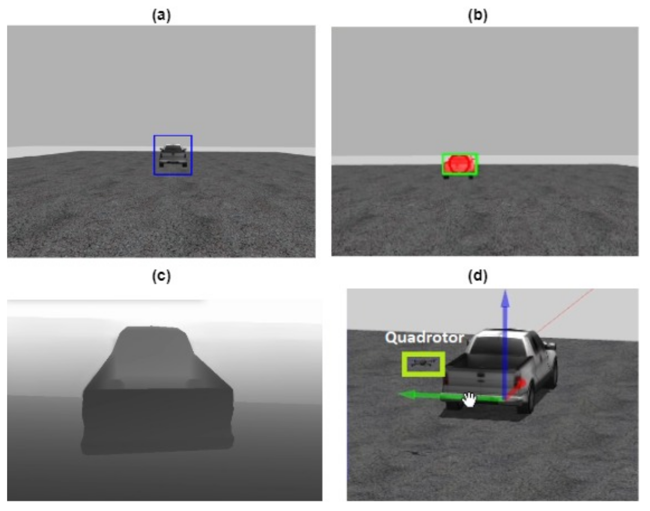
Figure 1. The visual tracker in the simulation environment. (a) The bounding-box area defines the target object for the tracker, (b) the single-object tracker is tracking the target, (c) the hybrid-depth map is generated in real time to supply the path planner with the position of the target each time step in the 3D space, and (d) the quadrotor moves toward the target until the quadrotor reaches to the object.
Remotesensing 14 05756 g001
Figure 2. Each case illustrates one of the main challenges in object tracking. (a) The ground truth is moving quickly, (b) the object is partially or completely hidden, (c) the background around the target object has the same color or texture as that object, and (d) the illumination in the target area has been dramatically affected.
Remotesensing 14 05756 g002
Figure 3. Schematic illustration for the problem formulation, where the multi-rotor tracks the moving object from the time step t 1 until it reaches the moving-object location. The red rectangles represent the moving object over time and the blue circles represent the center of the moving object. In our proposed online approach, we aim to achieve high practical convenience by combining visual tracking, object segmentation, and depth estimation. For initialization, the system relies on a simple bounding box initialization (the blue bounding box), produces an axis-aligned bounding box (the green bounding box), binary segmentation mask, and estimates the position of the object center. θ R 2 represents the multi-rotor’s camera field of view (fov). t i is the time step.
Remotesensing 14 05756 g003
Figure 4. Schematic illustration of the vision-based tracking system. Two FCNs with the same backbone f θ for RoW creation. The monocular depth estimation (MiDaS) works hand in hand with the input depth map to produce the hybrid-depth map. There are three main branches (mask, bounding box, and score) with an additional classifier. d denotes depth-wise cross correlation. The term H is defined by Equation (4). h ϕ is a simple two-layer network, while b σ , s γ are 1 × 1 convolutional layers.
Remotesensing 14 05756 g004
Figure 5. Hybrid-depth map. The figure shows how the proposed hybrid-depth map changes overtime. t is the frame number. The white arrows point to the borders between short range (depth estimation is measured by the sensor [42]) and the medium and long ranges (depth estimation is performed by the proposed hybrid-depth estimation algorithm).
Remotesensing 14 05756 g005
Figure 6. Simulation environments. (a) The basic simulation environment. There is the moving object, and the multi-rotor. (b) The customized simulation environment. There are three identical moving objects, the multi-rotor, one gas station, and a residential area with multiple houses, etc.
Remotesensing 14 05756 g006
Figure 7. Generic-tracker experiment result. In this experiment, the multi-rotor tracked the moving object until it reached the moving object. The figure shows that the multi-rotor almost passed the target position. The generic object tracker could cause instability in the tracking process because of the inherited behaviour of the Siamese network.
Remotesensing 14 05756 g007
Figure 8. Class-specific tracker. The figure shows the multi-rotor stopped right before the car. Unlike the generic tracker, the class-specific tracker can recognize the class of the target object, which makes the tracker performs the task of tracking as expected.
Remotesensing 14 05756 g008
Figure 9. Tracking the moving object. (a) The multi-rotor follows the moving object. (b) The multi-rotor stopped after reaching the target object.
Remotesensing 14 05756 g009
Figure 10. Tracking one of multiple moving objects. This experiment was performed in the customized simulation environment. The moving objects were distributed in the scene to try to confuse the object tracker.
Remotesensing 14 05756 g010
Figure 11. Results for tracking one of multiple identical moving objects; t is the frame number. The object tracker managed to keep tracking the target object without being confused by the other similar objects. The black trajectory is the estimated position of the moving object over time. The green trace is the prediction horizon generated by the local planner [56].
Remotesensing 14 05756 g011
Figure 12. Results for tracking a far moving object; t is the frame number. In this experiment, there was only one moving object in the scene. The multi-rotor made aggressive movements to simulate how the object tracker could behave in the existence of external factors (i.e., wind). The multi-rotor started to move aggressively towards the moving object at t = 5 , which explains why the object tracker did not correctly detect the target moving object at t = 5 and t = 10 . The tracker managed to track the moving object very well except at t = 5 and t = 10 .
Remotesensing 14 05756 g012
Figure 13. The depth estimation in the short range and the actual depth value.
Remotesensing 14 05756 g013
Figure 14. Medium range—(a) depth estimation and (b) error measurement.
Remotesensing 14 05756 g014
Figure 15. Long range—(a) depth estimation and (b) error measurement.
Remotesensing 14 05756 g015
Figure 16. The position error for medium and long ranges.
Remotesensing 14 05756 g016
Table 1. Summary of the state-of-the-art DL trackers with different attributes.
ApproachSpaceBackboneModulesLocalization MethodTraining SchemeInputFPSUpdateRedetection
M 2 -Track/2022 [7]3DPointNet-binary classification, BBRCross-entropy + Huber-loss + AdamLidar57no-updateN
3D-SiamRPN/2021 [40]3DPointNet-++-binary classification, BBRFocal-loss + Smooth L1-lossLidar20.8no-updateN
SiamGAT/2021 [44]2DGoogle-LeNetInception-V3binary classification, BBRBCE-loss+IoU loss+SGDRGB70no-updateN
TransT/2021 [45]2DResNet-50Block-4binary classification, BBRgiou loss+ L1-loss + cross-entropyRGB50no-updateN
P2B/20 [41]3DPointNet-++-binary classification, BBRBCE-loss + Huber-loss + AdamLidar40non-linearN
SiamR-CNN/2020 [46]2DResNet-101-FPNBlock-2,3,4,5binary classification, BBRBCE-loss + Huber loss + MomentumRGB4.7no-updateY
PrDiMP/2020 [47]2DResNet-18/50Block-4probabilistic density regression, IoU-predictionKL-divergence + loss steepest descent methodRGB30non-linearN
SiamMask/2019 [5]2DResNet-50Stage-1,2,3,4binary classification, BBR, logistic lossBCE-loss + SGDRGB55no-updateN
ATOM/2019 [32]2DResNet-18Block-3,4binary classification, BBRMSE + Adam(R), L2-loss + Conjugate Gradient(C)RGB30non-linearN
SiamRPN++/2019 [48]2DResNet-50Block-3,4,5binary classification, BBRBCE-loss + L1-loss + SGDRGB35no-updateN
SiamRPN/2018 [9]2Dmodified AlexNetconv5binary classification, BBRSmooth L1-Loss + BCE-loss + SGDRGB200no-updateN
DaSiam-RPN/2018 [6]2Dmodified AlexNetconv5binary classification, BBRSmooth L1-Loss + BCE-loss + SGDRGB160linearY
SiamFC/2017 [8]2DAlexNetconv5binary classification, scales searchinglogistic loss+SGDRGB86no-updateN
Table 3. Results for VOT-2016.
VOT-2016
EAO ↑Accuracy ↑Robustness ↓
SiamMask [5]0.4330.6390.214
The proposed generic tracker0.4330.6390.210
Table 4. Results for VOT-2019.
VOT-2019
EAO ↑Accuracy ↑Robustness ↓
The proposed generic tracker0.2810.6100.527
Table 5. Comparison with the state-of-the-art under the EAO, accuracy, and robustness metrics on VOT-2018. Up arrows indicate that bigger values are better. Down arrows indicate that smaller values are better.
EAO ↑Accuracy ↑Robustness ↓Speed (fps) ↑
The proposed generic tracker0.3810.610.28636
SiamMask [5]0.3800.6090.27655
DaSiamRPN [6]0.3260.5690.337160
SiamRPN [9]0.2440.4900.460200
SiamRPN++ [48]0.4140.6000.23435
PrDiMP [47]0.3850.6070.21740
CSRDCF [59]0.2630.4660.31848.9
SiamR-CNN [46]0.4080.6090.22015
THOR [60]0.4160.58180.234112
TrDiMP [33]0.4620.6000.14126
Publisher’s Note: MDPI stays neutral with regard to jurisdictional claims in published maps and institutional affiliations.