
Traffic Signal Optimization to Improve Sustainability: A Literature Review


1
CHA Consulting, 8935 NW 35th Ln, Doral, FL 33172, USA
2
Department of Civil & Environmental Engineering, Swanson School of Engineering, University of Pittsburgh, 341A Benedum Hall, 3700 O’Hara Street Pittsburgh, Pittsburgh, PA 15261, USA
*
Author to whom correspondence should be addressed.
Energies 2022, 15(22), 8452; https://doi.org/10.3390/en15228452
Submission received: 1 October 2022
/
Revised: 15 October 2022
/
Accepted: 26 October 2022
/
Published: 11 November 2022
(This article belongs to the Special Issue Vehicle Energy Consumption and Emissions in Intelligent and Sustainable Transportation Systems)
Abstract
:Optimizing traffic signals to improve traffic progression relies on minimizing mobility performance measures (e.g., delays and stops). However, delay and stop minimizations do not necessarily lead to minimal sustainability measures (e.g., fuel consumption and emissions). For that reason, researchers have focused, for decades, on integrating traffic models, signal optimization models, and fuel consumption and emissions models to minimize sustainability metrics while keeping acceptable levels of mobility metrics. Therefore, this paper reviews, classifies, and analyzes studies found in the literature regarding optimizing sustainable traffic signals. This paper provides researchers with a good starting point to further develop solutions which can address sustainable traffic control. To achieve that, this study details the most notable sustainable signal timing optimization studies from six perspectives: traffic models, fuel consumption and emissions models, optimization methods, objective functions, operating conditions, and reported sustainability savings. Outcomes of this research show that the previous studies deployed many combinations of elements from the six-perspective mentioned above, leading to a wide range of fuel consumption and emissions savings. The study also concludes that the available fuel consumption and emissions models are relatively old. Hence, future research is needed to develop new fuel consumption and emissions models based on recently collected data.
1. Introduction
Traffic congestion in current large metropolitan cities has been substantially increasing since the 1950s [1]. This can be primarily attributed to the enormous increase in vehicles’ private ownership due to rapid urbanization and economic growth. The primary issue with congestion is that it causes various externalities, including incidents, delays, and pollution. The increase in pollution affects human health, the globe, and the economy by increasing harmful pollutants, GHGs, and transportation expenditures. Although increasing transportation infrastructure capacity has been used to relieve congestion, researchers and experts realized that such a solution is costly and must be accompanied by operating existing capacity more efficiently.
Optimizing traffic signal timings is one of the critical strategies for addressing the congestion problem [2]. The first adjustments to traffic signal timings were made to make traveling safer, more reliable, and more convenient [3,4]. Later, other essential objectives (beyond safety) were sought when adjusting traffic signals, namely reducing delays and travel time by reducing the idling times and unnecessary stops [5]. The oil crisis of the early 1970s raised concerns about the amount of fuel consumed in traffic. This concern spread to all segments of traffic operations, and it eventually raised the question of how signalized intersections can be accommodated to minimize fuel consumption. Hence, nowadays, proper signal timing optimization is not only essential to regulate traffic flow, ease congestion, and improve mobility, but also acts as a valuable strategy to create a sustainable traffic environment.
Many signal timing optimization methods have been studied in the literature. The general theme of the previous studies encompasses deploying a traffic flow or simulation model and an optimization algorithm to optimize an objective function. As discussed later, the deployed traffic models can be microscopic, mesoscopic, and macroscopic in their detailing level. Optimization algorithms utilized in the traffic control problem seek to find the optimal values of one or more signal timing parameters (e.g., cycle length, offsets, splits, and phase sequence). Such optimal values result in the minimum or maximum output of the objective function. An objective function can include mobility (e.g., delay and stops) and/or sustainability (e.g., fuel consumption and emissions) measure(s).
Traffic signal optimization studies in the literature can be broadly classified based on their primary objective function into 1—mobility-based optimization, 2—sustainability-based optimization, and 3—multi-objective optimization, which seek to produce a balance between mobility and sustainability measures. What distinguishes the methodologies of signal optimization studies that involve improving sustainability from those studies seeking enhancing mobility is that the former includes fuel consumption and emissions models, which are not needed in the latter. Recent years (2015–2022) have seen a drastic increase in the studies concerning reducing sustainability measures by retiming traffic signals, as shown in Figure 1, which presents the distribution of the relevant studies by the publication year in the past two decades. However, the previous review articles focused mainly on the optimization algorithms used in the relevant literature (e.g., [6,7]). Moreover, there has not been a particular research effort to review the literature on signal optimization to improve sustainability measures. Therefore, this paper aims to comprehensively review, classify and analyze information found in the literature regarding sustainable traffic signals. This research attempts to provide researchers with a starting point to contribute solutions to the sustainable traffic signal problem.
It should be noted that this study focuses on the literature that optimized sustainability measures or those that evaluated sustainability metrics even if they used optimization of the mobility measures. Additionally, this research targets those studies with regular human-driven vehicles considered in the optimization. Studies with connected and autonomous vehicles are excluded because there is a large number of such studies in the literature, and thus such a study would warrant a separate research effort. In summary, 61 relevant studies are reviewed in this paper.
It should be also noted that long idling times in queues are one of the major causes of extra fuel consumption at signalized intersections. Some of the solutions include the estimation of the maximum queue size at the signal-controlled intersection approach (so-called: maximum back-of-queue) [8] and optimize traffic signal control modeling considering the number of vehicles in a queue [9].
In the past, studies usually focused on optimizing signal timings on isolated intersections. However, with the recent cutting-edge computational methods and high-fidelity modeling, it is feasible to optimize signals on relatively large-scale corridors considering various operating conditions (e.g., cruising speed and road gradient) that impact sustainability measures, especially in urban arterials. Consequently, researchers have recently started to focus more on exploring the impact of such operating conditions on the optimization results. In light of this introduction, this review article details the most notable sustainable signal timing optimization studies from six perspectives.
- The traffic model or simulation that was used to model traffic and obtain mobility performance metrics.
- The fuel consumption and/or emissions models used to evaluate the performance of the optimized signal plans from a sustainability point of view.
- The optimization algorithms are briefly reviewed and documented.
- The optimized objective functions.
- The reported fuel consumption and emissions saving (%) as representatives of sustainability.
The rest of the study is structured as follows: a recap of the early optimization efforts is presented in Section 2. Section 3 reviews traffic models and simulation programs. That section is followed by discussion of the fuel consumption and emissions models in Section 4. The optimization algorithms and their objective functions are analyzed and classified in Section 5. Relevant operating conditions and the reported savings are depicted in Section 6. Finally, future research and conclusions are provided in Section 7.
2. Early Efforts
In his seminal research, Webster [12] developed a method to optimize signal timings by minimizing vehicular delay (as the primary objective function), which became a basis for almost all subsequent similar studies. Robertson [13] was one of the first to computerize signal timing optimization, in TRANSYT, by using a performance index (PI)—a composite measure representing a linear function of delay and number of stops—to judge the quality of a set of signal timings. The release of the National Environmental Policy Act (NEPA) and the 1973 oil embargo attracted researchers to investigate the impact of traffic signals and their timings on fuel consumption and emissions. For example, Claffey [14] showed that traffic signals and several factors (such as cruising speed, pavement type, road gradient, and vehicle type) significantly impact vehicle fuel consumption and emissions. On the retiming side, Bauer [15] integrated an incremental fuel consumption model with SIGOP [16] and showed that the cycle length required to minimize fuel consumption at isolated intersections is longer than the one needed to minimize delay. Similar results were reported by Courage and Parapar [17], who also showed an apparent trade-off between travel delay and fuel consumption in the signal optimization problem, which can be achieved using TRANSYT model and its PI objective function. Cohen and Euler [18] used NETSIM (formerly UTCS-1) [19] and Emission Modal Analysis Model (EMAM) database [20] to conclude that delay, fuel consumption, and emissions are all minimized at the same cycle length. This conclusion disagreed with the results of others [15,17,21], which have found that fuel consumption is reduced when cycle lengths are longer than the ones required to minimize vehicular delay. Nevertheless, all of these research efforts were based on macroscopic kinematics and dynamics analysis and under inconsistent operating conditions (e.g., grades and vehicle types), which might have resulted in different conclusions.
Robertson et al. [22] quantified that 3% extra fuel consumption saving can be gained on coordinated signals through a trade-off between delay and stops using TRANSYT-7F’s PI. Such a trade-off (balance) was achieved by assigning a penalty of 20 s of delay time to each stop in the optimization problem. This influential work from Robertson et al. [22] set the stage for the PI to become a standard performance measure to optimize signal timings [11].
In summary, the early studies focused on using low-resolution analysis to achieve a balance between mobility and sustainability measures. The next batch of relevant studies focused on converting the signal control formulations into an optimization problem to balance mobility and sustainability [23,24,25,26]. After the mid-1980s, research interest in the impact of signal operations on fuel consumption and emissions has somewhat diminished. The revival of such research efforts occurred around the start of the new millennium (2000). Hence, the following sections review the most notable signal control optimization studies conducted between 2000 and 2022, which aimed to reduce fuel consumption and vehicular emissions.
3. Traffic Models or Simulation Software Programs
Traffic models are classified according to their level of detail into three categories: macroscopic (also known as deterministic or analytical), mesoscopic, and microscopic (also known as stochastic) [27]. Macroscopic models represent traffic as a flow defined by deterministic interrelationships between flow, speed, and density [27]. The measures of effectiveness (MOEs) from macroscopic models are aggregated based on the entire or part of an extensive traffic network at a time step higher than second-by-second (usually ≥ 5-min). Although macroscopic models require less computational load than mesoscopic and microscopic models, they have limited accuracy because they do not consider the variations in individual driving behavior between vehicles. Microscopic models use car-following and lane-changing models to simulate the travel trajectory of individual vehicles. MOEs from microscopic models can be provided over high-resolution time increments (e.g., one or a fraction of a second). One of the advantages of microscopic models is that they consider the impact of various operating conditions (e.g., driving behavior) on the vehicle’s kinematics (speed and acceleration). Mesoscopic models combine the two approaches of the macroscopic and microscopic models. Specifically, Mesoscopic models are developed in some respects similar to microscopic models (e.g., allow defining driving behavior) but aggregate MOEs at a section-by-section level similar to a macroscopic model. In summary, it is logical to conclude that macroscopic and mesoscopic models are more appropriate for planning studies, whereas microscopic are superior for operation studies (e.g., signal timing optimization).
Despite the above, researchers used two types of traffic modeling in the reviewed studies, which are analytical and microscopic models. Almost 36% of the models were analytical, and 64% were microscopic. Although the reviewed studies used many analytical models, the most implemented analytical models are the Webster model [12], Akçelik and Rouphail, 1993 [28], and the formulations of the Highway Capacity Manual (HCM) [29]. Such models are well-known in the literature for accurately representing traffic at a low computational cost. On the microscopic side, VISSIM [30] and SUMO [31] are the most deployed models, followed by AIMSUN [32], at a significantly lower rate. Other microscopic models were also deployed, as shown in Figure 2. Utilizing such models provides a much more accurate representation of traffic (compared to analytical models) by providing second-by-second vehicular trajectories that are immensely desirable when estimating fuel consumption and emissions [33,34].
Interestingly, most studies that focused on computerizing the traffic control optimization problem used an analytical models or SUMO. In contrast, most studies that focused on correctly modeling the traffic aspects of the problem have used microscopic models (e.g., VISSIM and AIMSUN). That can be explained by the fact that SUMO is an open-source model and has a friendly Application programming interface (API) for simulating traffic and transportation facilities [31], whereas VISSIM and AIMSUN require a subscription. Hence, if the study’s goal was to apply an optimization technique to a new problem, very accurate traffic modeling is not the highest priority. In addition, SUMO has an integrated fuel consumption and emissions model [35], which reduces the computation burden of utilizing an external fuel consumption and emissions model to evaluate the optimized signal timing plans compared to base case plans.
Figure 3 visualizes the traffic models or simulation programs with each study’s fuel consumption and emission models (discussed next) to provide readers with more specific information on the tools deployed by the reviewed studies. The traffic simulation or models (the first column from the left) is connected with the studies (the second column from the left) and the fuel consumption and/or emission model (the third column from the left), which have been used in the optimization process to assess the performance of the optimal signal timing plans. In summary, reviewed studies have deployed a large number of combinations of traffic and fuel consumption and emissions models. That might have led to various results and conclusions as discussed in Section 6.
4. Fuel Consumption and Emissions Models
Like traffic models, the current state of practice of fuel consumption and emissions models can also be divided into three categories according to their level of details. First, macroscopic (also known as elemental) models use averaged network or link-based inputs, mainly speed, to estimate network-wide or link-based fuel consumption and emission rates per unit distance (e.g., L/km). The major disadvantage of using macroscopic models is that they do not consider the instant changes in an individual vehicle’s speed and acceleration, which introduce an error in fuel consumption and emissions estimates. Such an error might be significant in urban arterials because of the stop-and-go events caused by signals. Second, mesoscopic models deal with smaller sections of the network than those of macroscopic models. However, they still ignore instantaneous variations in the vehicle’s kinematics. Third, microscopic models estimate second-by-second fuel consumption and emissions (in grams) based on second-by-second kinematic input variables (e.g., speed, acceleration, and road gradient). There are two types of microscopic models:
- Analytical models that are represented by one equation as a function of speed and acceleration (sometimes grade) for each sustainability measure (e.g., CO and HC). Such analytical models usually are developed based on a small number of vehicles; hence they group vehicles into 2–3 types (e.g., light-duty vehicles, Heavy-duty-vehicles, and sometimes buses or public transit). Although most analytical models are regression-based models, some of them are power-demand models. The main difference is that the former models are developed based on speed and acceleration data. In contrast, the latter models are developed based on the power required to increase a vehicle’s speed under a desired acceleration.
- Computerized models that share most of the analytical modes’ features except that they group vehicles with more details based on their fuel consumption and emissions characteristics. Such models usually have more than three vehicle types under each of the LDVs and HDVs categories.
Generally, it seems that evaluating an optimal set of signal timings would be most accurate if it was carried out by using microscopic models. That is because such models capture the enormous number of changes in speed and acceleration caused by the large number of deceleration-acceleration events entailed in the signal operation. For that reason, many of the reviewed studies (~76%) have employed microscopic models, as shown in Figure 4, to evaluate the results of their optimized signal plans. However, more than half of those studies (~56%) used analytical models that do not provide a wide range of vehicle types. Hence, their results can be considered less reliable than those studies that used computerized models and took advantage of the various vehicle types available in such studies. It is crucial to note that using a computerized model does not differ from using an analytical model unless a realistic vehicular fleet distribution is implemented. Unfortunately, few studies only integrated various vehicle types and fleet distributions in their analysis, as discussed later (Section 6).
Reviewing the fuel consumption and emissions models in the relevant literature revealed that all the studies (except one) that used SUMO as a traffic model have also used its integrated fuel consumption and emissions model (Handbook Emission Factors for Road Transport (HBEFA)) [35]. Like CMEM and VT-Micro, the HBEFA model considers the three primary modes of travel (acceleration, deceleration, and idling) to estimate fuel consumption and various emission types in grams per unit distance. Thus, HBEFA is the most implemented model in the reviewed studies, followed by CMEM and VT-Micro, at almost half the rate of the SUMO.
A handful of the reviewed studies used (Vehicle Specific Power) VSP-based fuel consumption and emissions models (e.g., MOVES [138] and fuel consumption and emissions model integrated with PARAMICS [44]). The concept of VSP was first introduced by Jimenez-Palacios [156] to overcome the inaccuracy of estimating fuel consumption and emission using elemental models. The idea of VSP-based models is to use fundamental physics to calculate the power per mass (e.g., W/kg) required for a specific speed, acceleration, and grade. The next step is to place each computed VSP value in a predefined VSP mode based on a predefined range of VSP values. For instance, if the VSP value is between 0 and 1, it belongs to mode 2. Finally, users can use another table to find the fuel consumption and emissions factors corresponding to the VSP mode.
Although VSP-based models can consider driving behavior and hence various emitting rates of emissions, such models still suffer from the fact that they use VSP modes that are based on VSP ranges (bins) to determine the fuel consumption and emissions factors (coefficient). For example, mode 4 of a VSP-based model has a range (bin) of 1 < = VSP < 4. Hence, a VSP of 1.1 W/kg has the same VSP mode as a VSP of 3.9, which results in the same fuel consumption and emissions factors for both VSP values. This apparently could introduce a significant margin of error that might impact the results and conclusions of a particular study.
A very small percentage of studies claim to use VISSIM to estimate fuel consumption and emissions in US gallons per distance. To the authors’ knowledge, however, VISSIM does not have its (integrated) fuel consumption and emissions model. Instead, VISSIM provides emission modeling with an External Model DLL. The original External Model DLL provided by VISSIM includes dummy fuel consumption and emissions models to be replaced with real models [30], as presented by Nouri and Morency, 2015 [157]. Hence, an inexperienced user of VISSIM might mistakenly believe that such dummy models can be used reliably. It is important to note that VISSIM has recently added a new Add-On module to compute emissions based on BOCSH models [158]. BOCSH models estimate emissions only and in grams per unit distance, not in US gallons per distance. However, the studies referred to earlier in this paragraph do not mention use of the BOCSH model. Hence, it seems that the results of those studies are less reliable than others.
Another issue found in the literature is unreferenced fuel consumption and emissions factors. A small percentage of studies report using what they call “commonly accepted fuel consumption and emissions factors” without proper references. Although the deployed factors might be common as claimed, such lack of referencing does not help enrich the literature and might mislead other researchers who are interested to follow such studies.
It should also be noted that despite all of the advancements in modeling fuel consumption models, a relatively significant percentage of studies still deployed elemental fuel consumption models, as shown in Figure 3. Although such models were state-of-the-art in modeling fuel consumption from the early 1980s until the mid-1990s, such models were repeatedly proven in the literature to have significantly less accurate estimates than microscopic models [159,160,161,162,163,164]. Therefore, the authors recommend that future studies should cease using elemental models to estimate fuel consumption and emissions.
In summary, the fuel consumption and emission models used in the reviewed studies are not maintained and are relatively old. Hence, there is a need to develop new models based on modern vehicular fleets to reflect the current fuel and energy consumption state followed by vehicle manufacturers. Such newly developed models are anticipated to provide an accurate estimation of the current impact of vehicles on environmental and health issues induced by vehicular emissions.
5. Optimization Techniques and Objective Functions
The reviewed studies in this research applied a large number of optimization techniques. The general theme of applied optimizations is to optimize an objective function(s) to improve sustainability and/or mobility measures (discussed next). The word ‘optimize’ in the reviewed studies often refers to minimizing or maximizing unwanted (e.g., delay and fuel consumption) or wanted (e.g., throughput of vehicles in the network, speed, and capacity) Measure of Effectiveness (MOEs), respectively. However, sometimes ‘optimize’ meant achieving a balance between mobility and sustainability measures. The optimization methods applied by studies presented in this research can be broadly classified into four techniques: 1—calculus-based using the first and second derivations, 2—guided random search (e.g., genetic algorithm (GA)) approach, 3—the enumerative technique as a common way to solve mixed-integer mathematical programs, and 4—machine learning-based optimization. Considering that reviewing optimization techniques requires a standalone effort, this effort is outside of this study’s scope. For the readers’ convenience, however, Figure 5 summarizes the optimization techniques (the first column from the left) applied in the reviewed studies (the second column from the left). Readers are referred to the relevant literature [6,7] for detailed information. Figure 5 (the third column from the left) also shows that reviewed studies have proposed and optimized many objective functions, which can be grouped as follows:
- Optimizing one or more mobility measures, mainly delay and number of stops. Such measures were usually computed and exported directly from the deployed traffic model for each potential optimal solution (signal plan) to evaluate its performance compared to the previous potential solution (or the base case).
- Optimizing a mobility performance index encompassing more than one mobility measure where each measure can be given a certain weight in the optimization. Such a performance index provides a balance between the conflicting mobility measures, namely delay and stops, as documented in several studies since the 1970s. Computing a performance index requires an extra step in addition to the computation done for the previous optimization above. This extra step is to multiply the weight of each mobility measure by its value as calculated by the traffic model. Hence, the primary criteria to determine the performance of the potential optimal solution is the performance index, not the mobility measure itself. At the end of the optimization, however, most studies evaluate the performance of the mobility measures values for the optimal solution compared to the base-case scenario (e.g., implemented in the field or optimized by a well-known optimization tool like Synchro).
- Optimizing one or more sustainability measures as the objective function. The focus in such an objective was often given to fuel consumption and carbon dioxide (CO2). This objective function requires deploying a fuel consumption and emission model to estimate their values for every potential solution based on the mobility measures provided by the traffic model. Thus, optimizing sustainability measures is more computationally demanding than the first two forms of objective functions. A drawback of using fuel consumption and emissions directly in the objective function is that applying such a function in the field is challenging. Another issue with this type of functions is that it might reduce sustainability metrics at the expense of worsening mobility metrics.
- Optimizing a performance index that consists of a combination of mobility and sustainability measures. Similar to optimization 2 above, weights can be given to various measures. This form of objective functions came to light when researchers recognized that minimizing mobility measures does not necessarily minimize sustainability measures. This type of functions has the same disadvantages mentioned above for optimization 3; mainly, it is time-consuming as it requires estimating sustainability measures for every potential solution.
- To reduce the computation burden in optimizations 3 and 4 above, the final form of objective functions is a performance index that consists of mobility measures only with sustainability-based weights given to one or more of those measures. This optimization requires computing sustainability measures twice instead of for every potential solution. The first time is when determining the sustainability-based weight(s) to be used in the optimization. The second time is when evaluating the optimal signal plan and comparing it with the base case scenario.
In summary, the reviewed studies have proposed and optimized many different forms of objective functions to improve sustainability. However, a few of those are actually implemented including the Performance Index (PI), which is the primary objective function in Synchro and Vistro. Hence, using such a PI with sustainability-based weight(s) might be beneficial.
6. Operating Conditions and Sustainability Savings
Traffic operating conditions affect vehicular fuel consumption and emissions [11]. Traffic operating conditions can be defined as the set of conditions under which vehicles operate individually and as a group. Such conditions include vehicle type, distribution of each vehicle type in the traffic fleet, cruising speed, road gradient, driving behavior, and ambient temperature, among others. Because of the significant impact of those operating conditions on sustainability, transportation engineers strive to reduce their sustainability costs by providing environmental solutions in transportation operations. Thus, it is vital to include the impact of various operating conditions when designing sustainable traffic signal control as one of the primary solutions to reduce fuel consumption and emissions footprints in urban areas.
For this reason, this section analyzes the reviewed studies based on the operating conditions considered in their optimizations, as presented in Table 1. Four operating conditions, which are vehicle type, fleet distribution, cruising speed, and grade, were included in the analyses. Those conditions were specifically chosen because of their substantial impact on fuel consumption and emissions, as documented by other studies [10,11]. Moreover, Table 1 in this section also indicates if a particular study took advantage of the emerging high-resolution (second-by-second) technology in their deployed fuel consumption and emissions computation. Finally, the reported savings in various sustainability measures are summarized and discussed in Table 2. Those measures are fuel consumption (FC), carbon monoxide (CO), carbon dioxide (CO2), and ‘volatile’ hydrocarbons (‘VOC’ and HC), nitrogen oxides (NOx), and particulate matters (PMs). It is worth noting that although there is a slight difference between VOC and HC, they are treated as a single emission type in this study because none of the reviewed studies distinguished between two of them.
Before commencing the discussion about vehicle type, it should be mentioned here that there are two major vehicular classifications. First is a high-level classification that groups vehicles into Light-duty vehicles (LDVs) and heavy-duty diesel vehicles (HDDVs). The fleet distribution column in Table 1 reflects whether the study included both categories in the high-level classification. The second is low-level (more detailed) classification, which groups vehicles subordinate to the LDVs and HDDVs. The vehicle type column in Table 1 reflects whether the study used multiple types of LDVs and documented the specifications of the utilized LDVs.
Although vehicle type is the most impactful factor on sustainability metrics [11], only ~18% of the reviewed studies documented using multiple LDVs, and the rest used one LDV type. Moreover, many studies did not precisely report the vehicle type(s) specification in their case studies. Such a lack of documentation of the tested vehicle types adds ambiguity to the results, preventing a meaningful comparison between various studies.
On the fleet distribution side, specifically the percentage of heavy vehicles in the fleet, only ~10% of the studies included heavy vehicles in their optimizations. It is worth mentioning that most of those studies did not disclose the percentage of heavy vehicles modeled in their case studies. Furthermore, none of the reviewed studies investigated the impact of various percentages of heavy vehicles in the optimization process on the savings and conclusions. That can be partially explained by the fact that such investigations are tedious and costly as they require performing many optimization scenarios.
Regarding road gradient, none of the previous studies included the impact of the road gradient, even though several studies documented significant implications for the percentage of grade on the sustainability metrics [165,166]. This gap can have significant adverse effects on the optimization results. For example, the optimizer might generate a ‘so-called’ optimal signal plan for level-terrain conditions on all links in the optimized corridor or network, whereas, in fact, many links in the optimized network have a particular slope. In such cases, the generated ‘optimal’ signal plan is not truly optimal.
Cruising speed is the second most impactful factor on fuel consumption and emissions [11]. Such an impact is most profound at signalized intersections because of the frequent stop-and-go events. All reviewed studies considered speed when estimating fuel consumption and emissions. However, such consideration was somehow forced by the fact that all fuel consumption and emissions models are functions of speed as the main parameters, among others. Hence, similar to the percentage of heavy vehicles, studies typically used a single cruising speed as the posted speed limit in the field without performing several optimization scenarios to evaluate the impact of speed on the optimization.
The second column from the left in Table 1 shows the studies that utilized high-resolution (second-by-second) sustainability estimates. The results uncovered that 62.3% of the reviewed studies had used microscopic sustainability metrics estimates. Those studies are considered more accurate than the rest because they captured the instantaneous change in cruising speed, resulting in accurate fuel consumption and emissions estimates, as discussed earlier in the paper. It is noteworthy that few studies that used microscopic traffic models, hence could utilize high-resolution mobility metrics estimates, have aggregated those estimates per 5 or 10 min and used them to compute average sustainability measures per timeframe per section of the road (aka link). Hence, using microscopic traffic models does not necessarily mean high-resolution sustainability metrics.
Table 2 shows that various studies reported that savings in sustainability measures could vary significantly. For example, such savings can be lower than 1% and reach up to ~50%. However, studies that have reported low savings (e.g., <10%) in the sustainability metrics are thought to be more accurate and acceptable. That is because they compared their optimized signal plan(s) with an optimized base case signal plan(s) instead of what is running in the field yet might be outdated. Another logical reason for such reasonable thinking is that more than 10% savings seem too high and difficult to accept when the underlying methodology lacks the necessary fidelity and data resolution. In summary, most studies were not tested in the field nor applied on multiple networks; thus, one should be cautious in relying on their results and conclusion. Especially since most studies did not consider the major operating conditions in the optimization, as discussed earlier.
One can see from Table 2 that some studies reported savings only for fuel consumption or emissions, whereas other studies reported savings for all sustainability metrics. Moreover, a few studies combined all emissions in the same savings percentage range. Such results are not supported by studies that reported a unique saving percentage for each sustainability metric. Hence, future research should contribute to confirming one of the two types of results.
The analysis of the results in Table 2 revealed that ~46% of the reviewed studies evaluated savings in fuel consumption, CO, and NOx. Slightly lower percentages with ~42.6% and 37.7% of the studies reported saving in CO2 and HC (VOC), respectively. Although PMs are maybe the most dangerous emission type on humans’ health [164], surprisingly, less than 10% of the studies evaluated the impact of the optimized plans on PMs. That can be attributed to the lack of PMs models in the literature since most of the available emissions models do not estimate PMs. Another reason can be that PMs are produced profoundly by heavy vehicles, which were not of considerable concern in all reviewed studies. Therefore, future research should address modeling PMs for all types of vehicles. Another future investigation is needed to accurately estimate the impact of traffic operation and optimization on PMs. Such efforts would be precious and appreciated in areas with high PMs concentrations.
7. Future Research and Conclusions
The importance of incorporating sustainability in all aspects of transportation has been increasing, which increases responsibility of transportation agencies to account for their environmental targets. To this end, this research reviews the most notable sustainable signal timing optimization studies. It is important to note that studies with connected and autonomous vehicles are excluded because there is a large number of such studies in the literature, and thus such a study would warrant a separate review effort. The studies were reviewed from six aspects: traffic models, fuel consumption and emissions model, optimization methods, objective functions, operating conditions, and reported sustainability savings. A careful analysis of the reviewed studies unfolded several conclusions and gaps in the existing literature. Hence, the following are the major conclusions and research areas that should be considered for future investigation:
- Most studies reviewed in this research optimized signal timings under either undocumented or under-saturated traffic conditions. Although a few studies covered multiple optimization scenarios based on three traffic conditions (light, moderate, and congested), those studies reached different conclusions. Specifically, one study concluded that the highest saving in sustainability measures could be achieved during congested conditions. In contrast, two other studies reported that moderate traffic conditions have the highest savings. Hence, the research on the impact of various traffic conditions on signal timing optimization to improve sustainability should be done to fill this gap in the literature.
- Many reviewed studies used an isolated hypothetical intersection with a simple phasing design to evaluate the proposed traffic signal optimization methods. The results of such methods cannot be reliable since their testbeds do not necessarily represent most of the signalized intersections in urban areas. In addition, most of the reviewed studies optimized signals for a relatively small network (e.g., less than 10 signalized intersections). For that reason, future endeavors should focus on microscopically modeling and optimizing real large-scale networks to evaluate the performance of the proposed optimization methods.
- Although online optimizations have proved their capability in several transportation applications [167], less than 5% of the reviewed studies have proposed using such optimizations for traffic signal control where focus is on the sustainability. Future research directions should investigate the ability to simulate large networks with real-time data to fill this void in the literature.
- The research on multi-sustainability-objectives optimizing traffic signals is not significant. Thus, future research should study multi-sustainability objective that includes more measures in addition to fuel consumption and emissions. For example, safety, noise, and pedestrian and cyclists’ exposure to vehicle emissions using emissions dispersion models. The idea here is not that all objectives act simultaneously, but various times of day or year (e.g., seasons) can have different optimization strategies. For example, optimizing noise can be the objective during the night.
- The majority of the optimization algorithms proposed in the reviewed papers have performed well. However, they were time-consuming and required intensive computational loads. Although some optimization techniques were introduced to reduce the computational load of other optimizations, they still consume more time and processing loads than what might be practical to apply in the field. Thus, more efficient computational techniques should be addressed in future studies.
- There is a tradition found in the reviewed literature, to optimize one or two signal parameters (e.g., cycle length and offset). This finding can be partially explained by the fact that transportation agencies do not prefer changing some signal parameters (e.g., phase sequence from lead to lag or vice versa) in a particular area. A few studies broke that tradition and showed that optimizing all four signal parameters can be more beneficial than optimizing a single parameter. However, those studies did not investigate the interrelationship between the different signal parameters. Hence, future research should address the impact of optimizing signal parameters on each other’s values. Such research can offer flexible signal control strategies in the future.
- The bulk of the signal optimization techniques, and their alternatives of reinforcement learning approaches (e.g., [168,169,170,171]) introduced by the previous studies, are not adopted by transportation agencies, partially because of their complexity. Moreover, many recent studies proposed optimization models for mixed vehicular fleets (CAVs and human-driven vehicles) and showed significant sustainable benefits obtained by employing autonomous vehicles e.g., [172,173]. However, such studies need a relatively long time to be implemented in the field. Therefore, there is an urgent need, originated by the accelerating change in the climate, for more technologies based on today’s average vehicles, traffic signals, and the optimization tools utilized by transportation agencies.
- A great deal of fuel consumption and emissions models were deployed in the literature, and such deployment did not exceed the application limit. Specifically, reviewed studies used the models without any calibration or validation efforts to their estimations in the area of optimized signal(s). This practice can introduce a significant error, especially when using a model for an area with very different characteristics than that where the model was originally developed. Hence, future work should be centered on calibrating and validating various fuel consumption and emissions models. Furthermore, the available fuel consumption and emissions models are relatively old to be applied in a modern vehicular fleet. A new model development effort should look into utilizing the enormous prediction capability of machine learning techniques to develop modern fuel consumption and emissions models. That is especially needed for the estimation of particulate matters produced by heavy vehicles.
- Although a few studies realized the importance of including the impact of various operating conditions (e.g., vehicle type) in the optimization problem, a limited number of studies considered multiple vehicle types. In addition, none of the reviewed studies considered the impact of road gradients or other factors (e.g., driving behavior) influencing sustainability measures. Therefore, the optimization results and conclusions may differ when various vehicle types, fleet distributions, acceleration-deceleration functions, and other impactful factors are involved. Therefore, future research should investigate the individual and combined impacts of multiple operating conditions on the optimization results.
Author Contributions
Conceptualization, S.A. and A.S.; methodology, S.A., A.S., N.M.; formal analysis, S.A. and N.M.; investigation, S.A., N.M., A.S.; resources, S.A. and E.E.; writing—original draft preparation, S.A.; writing—review and editing, A.S., N.M., E.E.; visualization, S.A.; All authors have read and agreed to the published version of the manuscript.
Funding
This research received no external funding.
Data Availability Statement
Not applicable.
Conflicts of Interest
The authors declare no conflict of interest.
References
- Caves, R.W. Encyclopedia of the City; Routledge: London, UK, 2004. [Google Scholar]
- Systematics, C. Traffic Congestion and Reliability: Linking Solutions to Problems (No. FHWA-HOP-05-004); Federal Highway Administration: DC, USA, 2004. [Google Scholar]
- Matson, T.M. The Principles of Traffic Signal Timing; Yale University: New Haven, CT, USA, 1939. [Google Scholar]
- Clayton, A.J.H. Road Traffic Calculations. J. Inst. Civ. Eng. 1941, 16, 247–264. [Google Scholar] [CrossRef]
- Gazis, D.C. Traffic Theory (Vol. 50); Springer Science & Business Media: Berlin/Heidelberg, Germany, 2006. [Google Scholar]
- Sawake, V.V.; Borkar, P. Review of traffic signal timing optimization based on fuzzy logic controller. In Proceedings of the 2017 International Conference on Innovations in Information, Embedded and Communication Systems (ICIIECS), Coimbatore, India, 17–18 March 2017; p. 4. [Google Scholar]
- Hale, D.K.; Park, B.B.; Stevanovic, A.; Su, P.; Ma, J. Optimality versus run time for isolated signalized intersections. Transp. Res. Part C Emerg. Technol. 2015, 55, 191–202. [Google Scholar] [CrossRef]
- Macioszek, E.; Iwanowicz, D. A back-of-queue model of a signal-controlled intersection approach developed based on analysis of vehicle driver behavior. Energies 2021, 14, 1204. [Google Scholar] [CrossRef]
- An, H.K.; Awais Javeed, M.; Bae, G.; Zubair, N.; Metwally, M.A.S.; Bocchetta, P.; Na, F.; Javed, M.S. Optimized Intersection Signal Timing: An Intelligent Approach-Based Study for Sustainable Models. Sustainability 2022, 14, 11422. [Google Scholar] [CrossRef]
- Stevanovic, A.; Shayeb, S.A.; Patra, S.S. Fuel Consumption Intersection Control Performance Index. Transp. Res. Rec. 2021, 2675, 690–702. [Google Scholar] [CrossRef]
- Alshayeb, S.; Stevanovic, A.; Dobrota, N. Impact of Various Operating Conditions on Simulated Emissions-Based Stop Penalty at Signalized Intersections. Sustainability 2021, 13, 10037. [Google Scholar] [CrossRef]
- Webster, F.V. Traffic Signal Settings; (No. 39); The National Academies of Sciences, Engineering, and Medicine: Washington, DC, USA, 1958. [Google Scholar]
- Robertson, D.I. TRANSYT: A Traffic Network Study Tool; The National Academies of Sciences, Engineering, and Medicine: Washington, DC, USA, 1969. [Google Scholar]
- Claffey, P.J. Running Costs of Motor Vehicles as Affected by Road Design and Traffic; NCHRP Report; The National Academies of Sciences, Engineering, and Medicine: Washington, DC, USA, 1971; p. 111. [Google Scholar]
- Bauer, C.S. Some energy considerations in traffic signal timing. Traffic Eng. 1975, 45, 19–25. [Google Scholar]
- Peat, Marwick, Livingston, Co. SIGOP Traffic Signal Optimization Program: User’s Manual; U.S. Dept. of Transport, Bureau of Public Roads: Washington, DC, USA, 1968. [Google Scholar]
- Courage, K.G.; Parapar, S.M. Delay and fuel consumption at traffic signals. Traffic Eng. 1975, 45, 23–27. [Google Scholar]
- Cohen, S.L.; Euler, G. Signal Cycle Length and Fuel Consumption and Emissions (No. HS-025 846); Transportation Research Board; The National Academies of Sciences, Engineering, and Medicine: Washington, DC, USA, 1978. [Google Scholar]
- Worrall, R.D.; Lieberman, E.B. Network Flow Simulation for Urban Traffic Control Systems-Phase II; Federal Highway Administration, National Technical Information Service: Springfield, VA, USA, 1973. [Google Scholar]
- Kunselman, P. Automobile Exhaust Emission Modal Analysis Model; Environmental Protection Agency, Office of Air and Water Programs, Office of Mobile Source Air Pollution Control, Certification and Surveillance Division: Ann Arbor, MI, USA, 1974. [Google Scholar]
- Hurley, J.W., Jr.; Ball, R.P. Evaluation of energy-based signal setting for traffic actuated control. In Modeling and Simulation: Proceedings of the Annual Pittsburgh Conference; Instrument Society of America: Pittsburgh, PA, USA; Volume 10, pp. 14–21.
- Robertson, D.I.; Lucas, C.F.; Baker, R.T. Coordinating Traffic Signals to Reduce Fuel Consumption (No. LR 934 Monograph); The National Academies of Sciences, Engineering, and Medicine: Washington, DC, USA, 1980. [Google Scholar]
- Al-Khalili, A.; El-Hakeem, A.K. A computer control system for minimization of fuel consumption in urban traffic network. In IEEE Real Time Systems Symposium; IEEE: New York, NY, USA, 1984; pp. 249–254. [Google Scholar]
- Al-Khalili, A.J. Urban traffic control—A general approach. In IEEE Transactions on Systems, Man, and Cybernetics; IEEE: New York, NY, USA, 1985; pp. 260–271. [Google Scholar]
- Reljic, S.; Kamhi-Barna, M.; Stojanovic, S. Multicriteria signal plan choice at an isolated intersection. In Mathematics in Transport Planning and Control; Institute of Mathematics & its Applications Conference Series 38; The National Academies of Sciences, Engineering, and Medicine: Washington, DC, USA, 1992. [Google Scholar]
- Foy, M.D.; Benekohal, R.F.; Goldberg, D.E. Signal timing determination using genetic algorithms. Transp. Res. Rec. 1992, 1365, 108. [Google Scholar]
- Jeannotte, K.; Chandra, A.; Alexiadis, V.; Skabardonis, A. Traffic Analysis Toolbox Volume II: Decision Support Methodology for Selecting Traffic Analysis Tools (No. FHWA-HRT-04-039); The National Academies of Sciences, Engineering, and Medicine: Washington, DC, USA, 2004. [Google Scholar]
- Akçelik, R.; Rouphail, N.M. Estimation of delays at traffic signals for variable demand conditions. Transp. Res. Part B Methodol. 1993, 27, 109–131. [Google Scholar] [CrossRef]
- Manual, H.C. Highway Capacity Manual; Transportation Research Board: Washington, DC, USA, 2000; Volume 2. [Google Scholar]
- PTV. VISSIM 2020 User Manual; PTV AG: Karlsruhe, Germany, 2020. [Google Scholar]
- Krajzewicz, D.; Erdmann, J.; Behrisch, M.; Bieker, L. Recent development and applications of SUMO-Simulation of Urban MObility. Int. J. Adv. Syst. Meas. 2012, 5, 128–138. [Google Scholar]
- TSS. AIMSUN 6.1 Microsimulator Users Manual; Transport Simulation Systems: Barcelona, Spain, 2011. [Google Scholar]
- Scora, G.; Barth, M. Comprehensive Modal Emissions Model (cmem), Version 3.01. User Guide; Centre for Environmental Research and Technology, University of California: Riverside, CA, USA, 2006; Volume 1070, p. 1580. [Google Scholar]
- Rakha, H.; Ahn, K.; Trani, A. Development of VT-Micro model for estimating hot stabilized light duty vehicle and truck emissions. Transp. Res. Part D Transp. Environ. 2004, 9, 49–74. [Google Scholar] [CrossRef]
- Infras, A.G. Handbuch für Emissionsfaktoren des Strassenverkehrs; Version 2.1; Bundesamt für Umwelt, Wald und Landschaft (BUWAL): Bern, Switzerland, 2004. [Google Scholar]
- van Vliet, D. SATURN Manual, 11th ed.; University of Leeds: Leeds, UK, 2018. [Google Scholar]
- Osorio, C.; Bierlaire, M. An analytic finite capacity queueing network model capturing the propagation of congestion and blocking. Eur. J. Oper. Res. 2009, 196, 996–1007. [Google Scholar] [CrossRef]
- Chen, X.; Osorio, C.; Santos, B.F. Simulation-based travel time reliable signal control. Transp. Sci. 2019, 53, 523–544. [Google Scholar] [CrossRef]
- Dong, Y. Research on Calculation Method and Optimal Control Strategy of Trffic Delay in Crosswalk. Ph.D. Thesis, Beijing Jiaotong Univeristy, Beijing, China, 2016. [Google Scholar]
- Treiber, M.; Kesting, A. Traffic flow dynamics: Data, models and simulation. Phys. Today 2014, 67, 54. [Google Scholar]
- Pipes, L.A. An operational analysis of traffic dynamics. J. Appl. Phys. 1953, 24, 274–281. [Google Scholar] [CrossRef]
- Bando, M.; Hasebe, K.; Nakayama, A.; Shibata, A.; Sugiyama, Y. Dynamical model of traffic congestion and numerical simulation. Phys. Rev. E 1995, 51, 1035. [Google Scholar] [CrossRef]
- Husch, D.; Albeck, J. SimTraffic 6 User Guide; Trafficware Corporation: Albany, CA, USA, 2003. [Google Scholar]
- Paramics, Q. The Paramics Manuals, Version 6.6.1; Quastone Paramics Ltd.: Edinburgh, UK, 2009.
- Integration Release 2.30 for Windows: User’s Guide; Van Aerde and Associates, Ltd.: Blacksburg, VA, USA, 2003.
- Nagel, K.; Schreckenberg, M. A cellular automaton model for freeway traffic. J. De Phys. I 1992, 2, 2221–2229. [Google Scholar] [CrossRef]
- Wu, B.; Li, Y. Traffic Management and Control; China Communication: Beijing, China, 2009; Volume 26. [Google Scholar]
- Yang, X.G. Manual of Urban Traffic Design; China Communications: Beijing, China, 2003. [Google Scholar]
- Axhausen, W.K.; Horni, A.; Nagel, K. The Multi-Agent Transport Simulation MATSim; Ubiquity Press: London, UK, 2016; p. 618. [Google Scholar]
- Treiber, M.; Hennecke, A.; Helbing, D. Congested traffic states in empirical observations and microscopic simulations. Phys. Rev. E 2000, 62, 1805. [Google Scholar] [CrossRef] [Green Version]
- Lighthill, M.J.; Whitham, G.B. On kinematic waves II. A theory of traffic flow on long crowded roads. Proc. R. Soc. Lond. Ser. A Math. Phys. Sci. 1955, 229, 317–345. [Google Scholar]
- Bert, E.; Dumont, A.G. Simulation de l’agglomération lausannoise, SIMLO (No. REP_WORK); EPFL Scientific Publications: Lausanne, Switzerland, 2006. [Google Scholar]
- Wallace, C.E.; Courage, K.G.; Reaves, D.P.; Schoene, G.W.; Euler, G.W. TRANSYT-7F User’s Manual (No. UF-TRC-U32 FP-06/07); University of Florida Press: Gainesville, FL, USA, 1984. [Google Scholar]
- Hale, D. Traffic Network Study Tool–TRANSYT-7F, United States Version. Mc-Trans Center in the University of Florida. Nat. Resour. 2005, 2. [Google Scholar]
- Liao, T.Y.; Hu, T.Y.; Chen, L.W.; Ho, W.M. Development and empirical study of real-time simulation-based dynamic traffic assignment model. J. Transp. Eng. 2010, 136, 1008–1020. [Google Scholar] [CrossRef]
- Daganzo, C.F. The cell transmission model: A dynamic representation of highway traffic consistent with the hydrodynamic theory. Transp. Res. Part B Methodol. 1994, 28, 269–287. [Google Scholar] [CrossRef]
- Daganzo, C.F. The cell transmission model, part II: Network traffic. Transp. Res. Part B Methodol. 1995, 29, 79–93. [Google Scholar] [CrossRef]
- Early Deployment of Transims. 1999. Available online: https://web.archive.org/web/20100527134930/http://tmip.fhwa.dot.gov/resources/clearinghouse/docs/issue_paper/issue_paper.pdf. (accessed on 1 October 2022).
- Shiwu, L.; Yunpeng, W.; Jianping, F. Signal timing optimization simulation on urban road intersection based on vehicle emissions. J. Ji Lin Univ. (Eng. Technol. Ed.) 2007, 37, 1268–1272. [Google Scholar]
- Lei, S.; Xiaohong, G.; Hanping, J. Urban microscopic traffic flow modeling and simulation. J.-Wuhan Transp. Univ. 2003, 27, 499–502. [Google Scholar]
- Akcelik, R. New Approximate Expressions for Delay, Stop Rate and Queue Length at Isolated Signals; Inist-CNRS: Paris, France, 1982. [Google Scholar]
- ITT Industries, Inc. CORSIM Reference Manual: Version 5.0; Systems Division and ATMS R&D and Systems Engineering Program Team, ITT Industries: Colorado Springs, CO, USA, 2001. [Google Scholar]
- Akçelik, R.; Besley, M. Sidra-2 User Guide; The National Academies of Sciences, Engineering, and Medicine: Washington, DC, USA, 1984. [Google Scholar]
- Horiguchi, R.; Katakura, M.; Akahane, H.; Kuwahara, M. A development of a traffic simulator for urban road networks: AVENUE. In Proceedings of the VNIS’94-1994 Vehicle Navigation and Information Systems Conference, Yokohama, Japan, 31 August–2 September 1994; pp. 245–250. [Google Scholar]
- Kosonen, I. HUTSIM-Urban Traffic Simulation and Control Model: Principles and Applications; The National Academies of Sciences, Engineering, and Medicine: Washington, DC, USA, 1999; Volume 100. [Google Scholar]
- Kővári, B.; Pelenczei, B.; Aradi, S.; Bécsi, T. Reward Design for Intelligent Intersection Control to Reduce Emission. IEEE Access 2022, 10, 39691–39699. [Google Scholar] [CrossRef]
- Li, M.; Luo, D.; Liu, B.; Zhang, X.; Liu, Z.; Li, M. Arterial coordination control optimization based on AM–BAND–PBAND model. Sustainability 2022, 14, 10065. [Google Scholar] [CrossRef]
- Zhang, X.; Fan, X.; Yu, S.; Shan, A.; Fan, S.; Xiao, Y.; Dang, F. Intersection Signal Timing Optimization: A Multi-Objective Evolutionary Algorithm. Sustainability 2022, 14, 1506. [Google Scholar] [CrossRef]
- Jovanović, A.; Stevanović, A.; Dobrota, N.; Teodorović, D. Ecology based network traffic control: A bee colony optimization approach. Eng. Appl. Artif. Intell. 2022, 115, 105262. [Google Scholar] [CrossRef]
- Ounoughi, C.; Touibi, G.; Yahia, S.B. EcoLight: Eco-friendly Traffic Signal Control Driven by Urban Noise Prediction. In International Conference on Database and Expert Systems Applications; Springer: Cham, Switzerland, 2022; pp. 205–219. [Google Scholar]
- Abudayyeh, D.; Nicholson, A.; Ngoduy, D. Traffic signal optimisation in disrupted networks, to improve resilience and sustainability. Travel Behav. Soc. 2021, 22, 117–128. [Google Scholar] [CrossRef]
- Chen, X.; Jia, Y. Sustainable traffic management and control system for arterial with contraflow left-turn lanes. J. Clean. Prod. 2021, 280, 124256. [Google Scholar] [CrossRef]
- Lin, H.; Han, Y.; Cai, W.; Jin, B. Traffic signal optimization based on fuzzy control and differential evolution algorithm. IEEE Trans. Intell. Transp. Syst. 2022, 1–12. [Google Scholar] [CrossRef]
- Feng, B.; Lin, Y.; Xu, J. A comprehensive traffic ecological performance index based on individual car and bus travel speed in urban road network. Resil. Sustain. Transp. Syst. 2020, 666–672. [Google Scholar]
- Bai, K.; Yao, E.; Pan, L.; Li, L.; Chen, W. Dynamic crosswalk signal timing optimization model considering vehicle and pedestrian delays and fuel consumption cost. Sustainability 2020, 12, 689. [Google Scholar] [CrossRef] [Green Version]
- Chen, X.; Yuan, Z. Environmentally friendly traffic control strategy-A case study in Xi’an city. J. Clean. Prod. 2020, 249, 119397. [Google Scholar] [CrossRef]
- Elidrissi, H.L.; Nait-Sidi-Moh, A.; Tajer, A. Knapsack problem-based control approach for traffic signal management at urban intersections: Increasing smooth traffic flows and reducing environmental impact. Ecol. Complex. 2020, 44, 100878. [Google Scholar] [CrossRef]
- Paul, A.; Mitra, S. Deep reinforcement learning based traffic signal optimization for multiple intersections in ITS. In Proceedings of the 2020 IEEE International Conference on Advanced Networks and Telecommunications Systems (ANTS), New Delhi, India, 14–17 December 2020; pp. 1–6. [Google Scholar]
- Song, Z.R.; Zang, L.L.; Zhu, W.X. Study on minimum emission control strategy on arterial road based on improved simulated annealing genetic algorithm. Phys. A Stat. Mech. Its Appl. 2020, 537, 122691. [Google Scholar] [CrossRef]
- Al-Turki, M.; Jamal, A.; Al-Ahmadi, H.M.; Al-Sughaiyer, M.A.; Zahid, M. On the potential impacts of smart traffic control for delay, fuel energy consumption, and emissions: An NSGA-II-based optimization case study from Dhahran, Saudi Arabia. Sustainability 2020, 12, 7394. [Google Scholar] [CrossRef]
- Wu, S.; Sun, K.; Liu, L. Urban Traffic Signal Timing Optimization by Reducing Vehicle Emissions. In Proceedings of the 2020 International Conference on Urban Engineering and Management Science (ICUEMS), Zhuhai, China, 24–26 April 2020; pp. 361–369. [Google Scholar]
- Calle-Laguna, A.J.; Du, J.; Rakha, H.A. Computing optimum traffic signal cycle length considering vehicle delay and fuel consumption. Transp. Res. Interdiscip. Perspect. 2019, 3, 100021. [Google Scholar] [CrossRef]
- Chen, H.; Chen, H.; Sun, Q. Study on the Optimization and Evaluation of Signalized Intersections Based on the Emission Analysis. In Proceedings of the 19th COTA International Conference of Transportation Professionals, Nanjing, China, 6–8 July 2019; pp. 1859–1868. [Google Scholar]
- Jia, H.; Lin, Y.; Luo, Q.; Li, Y.; Miao, H. Multi-objective optimization of urban road intersection signal timing based on particle swarm optimization algorithm. Adv. Mech. Eng. 2019, 11, 1687814019842498. [Google Scholar] [CrossRef] [Green Version]
- Li, X.; Sun, J.Q. Intersection multi-objective optimization on signal setting and lane assignment. Phys. A Stat. Mech. Its Appl. 2019, 525, 1233–1246. [Google Scholar] [CrossRef]
- Wang, Q.; Wang, K.; Zhou, S.; Shi, Q.; Sun, H. Signal timing optimization model of urban road intersection based on multi-factor. In Proceedings of the 2018 6th International Conference on Traffic and Logistic Engineering (ICTLE 2018), MATEC Web of Conferences. 3–5 August 2018; EDP Sciences; Volume 259, p. 02004. [Google Scholar]
- Zheng, L.; Xu, C.; Jin, P.J.; Ran, B. Network-wide signal timing stochastic simulation optimization with environmental concerns. Appl. Soft Comput. 2019, 77, 678–687. [Google Scholar] [CrossRef]
- Balta, M.; Özcelik, I. Traffic Signaling Optimization for Intelligent and Green Transportation in Smart Cities. In Proceedings of the 2018 3rd International Conference on Computer Science and Engineering (UBMK), Sarajevo, Bosnia and Herzegovina, 20–23 September 2018; pp. 31–35. [Google Scholar]
- Yao, R.; Wang, X.; Xu, H.; Lian, L. Emission factor calibration and signal timing optimisation for isolated intersections. IET Intell. Transp. Syst. 2018, 12, 158–167. [Google Scholar] [CrossRef]
- Kou, W.; Chen, X.; Yu, L.; Gong, H. Multiobjective optimization model of intersection signal timing considering emissions based on field data: A case study of Beijing. J. Air Waste Manag. Assoc. 2018, 68, 836–848. [Google Scholar] [CrossRef] [PubMed] [Green Version]
- Péres, M.; Ruiz, G.; Nesmachnow, S.; Olivera, A.C. Multiobjective evolutionary optimization of traffic flow and pollution in Montevideo, Uruguay. Appl. Soft Comput. 2018, 70, 472–485. [Google Scholar] [CrossRef]
- Shen, Y. An optimization model of signal timing plan and traffic emission at intersection based on Synchro. IOP Conf. Ser. Earth Environ. Sci. 2018, 189, 062002. [Google Scholar] [CrossRef]
- Abdelghaffar, H.M.; Yang, H.; Rakha, H.A. Developing a de-centralized cycle-free nash bargaining arterial traffic signal controller. In Proceedings of the 2017 5th IEEE International Conference on Models and Technologies for Intelligent Transportation Systems (MT-ITS), Naples, Italy, 26–28 June 2017; pp. 544–549. [Google Scholar]
- Armas, R.; Aguirre, H.; Daolio, F.; Tanaka, K. Evolutionary design optimization of traffic signals applied to Quito city. PLoS ONE 2017, 12, e0188757. [Google Scholar] [CrossRef]
- Ji, Y.; Hu, B.; Hill, G.; Guo, W.; Blythe, P.; Gao, L. Signal coordination scheme based on traffic emission. IET Intell. Transp. Syst. 2016, 10, 89–96. [Google Scholar] [CrossRef] [Green Version]
- Yu, D.; Tian, X.; Xing, X.; Gao, S. Signal timing optimization based on fuzzy compromise programming for isolated signalized intersection. Math. Probl. Eng. 2016, 2016, 1682394. [Google Scholar] [CrossRef]
- Haberl, M.; Fellendorf, M.; Dippold, M.; Furian, N.; Hausberger, S. Monitoring and optimizing coordinated signal control. In Proceedings of the 23rd ITS World Congress, Melbourne, VIC, Australia, 10–14 October 2016; 2016. [Google Scholar]
- Han, K.; Liu, H.; Gayah, V.V.; Friesz, T.L.; Yao, T. A robust optimization approach for dynamic traffic signal control with emission considerations. Transp. Res. Part C Emerg. Technol. 2016, 70, 3–26. [Google Scholar] [CrossRef] [Green Version]
- Tanaka, K. Traffic Signal Optimization: Minimizing Travel Time and Fuel Consumption. In Artificial Evolution: Proceedings of the 12th International Conference, Evolution Artificielle, EA 2015, Lyon, France, 26–28 October 2015; Revised Selected Papers; Springer: Berlin/Heidelberg, Germany, 2016; Volume 9554, p. 29. [Google Scholar]
- Khalighi, F.; Christofa, E. Emission-based signal timing optimization for isolated intersections. Transp. Res. Rec. 2015, 2487, 1–14. [Google Scholar] [CrossRef]
- Lin, C.; Gong, B.; Qu, X. Low emissions and delay optimization for an isolated signalized intersection based on vehicular trajectories. PLoS ONE 2015, 10, e0146018. [Google Scholar] [CrossRef] [PubMed]
- Olivera, A.C.; García-Nieto, J.M.; Alba, E. Reducing vehicle emissions and fuel consumption in the city by using particle swarm optimization. Appl. Intell. 2015, 42, 389–405. [Google Scholar] [CrossRef]
- Osorio, C.; Nanduri, K. Urban transportation emissions mitigation: Coupling high-resolution vehicular emissions and traffic models for traffic signal optimization. Transp. Res. Part B Methodol. 2015, 81, 520–538. [Google Scholar] [CrossRef]
- Osorio, C.; Nanduri, K. Energy-efficient urban traffic management: A microscopic simulation-based approach. Transp. Sci. 2015, 49, 637–651. [Google Scholar] [CrossRef] [Green Version]
- Li, P.; Mirchandani, P.; Zhou, X. Simulation-based traffic signal optimization to minimize fuel consumption and emission: A Lagrangian relaxation approach (No. 15-2358). In Proceedings of the Transportation Research Board 94th Annual Meeting, Washington, DC, USA, 11–15 January 2015. [Google Scholar]
- Stevanovic, A.; Stevanovic, J.; So, J.; Ostojic, M. Multi-criteria optimization of traffic signals: Mobility, safety, and environment. Transp. Res. Part C Emerg. Technol. 2015, 55, 46–68. [Google Scholar] [CrossRef] [Green Version]
- Dias, J.C.; Machado, P.; Silva, D.C.; Abreu, P.H. An inverted ant colony optimization approach to traffic. Eng. Appl. Artif. Intell. 2014, 36, 122–133. [Google Scholar] [CrossRef]
- Garcia-Nieto, J.; Ferrer, J.; Alba, E. Optimising traffic lights with metaheuristics: Reduction of car emissions and consumption. In Proceedings of the 2014 International Joint Conference on Neural Networks (IJCNN), Beijing, China, 6–11 July 2014; pp. 48–54. [Google Scholar]
- Ma, X.; Jin, J.; Lei, W. Multi-criteria analysis of optimal signal plans using microscopic traffic models. Transp. Res. Part D Transp. Environ. 2014, 32, 1–14. [Google Scholar] [CrossRef] [Green Version]
- Almasri, E.H. Signal coordination for saving energy and reducing congestion using transyt-7f model and its application in gaza city. Nat. Resour. 2014, 2014. [Google Scholar] [CrossRef]
- Zhou, Z.; Cai, M. Intersection signal control multi-objective optimization based on genetic algorithm. J. Traffic Transp. Eng. 2014, 1, 153–158. [Google Scholar]
- Liao, T.Y. A fuel-based signal optimization model. Transp. Res. Part D Transp. Environ. 2013, 23, 1–8. [Google Scholar] [CrossRef]
- Lv, J.; Zhang, Y.; Zietsman, J. Investigating emission reduction benefit from intersection signal optimization. J. Intell. Transp. Syst. 2013, 17, 200–209. [Google Scholar] [CrossRef]
- Qian, R.; Lun, Z.; Wenchen, Y.; Meng, Z. A traffic emission-saving signal timing model for urban isolated intersections. Procedia-Soc. Behav. Sci. 2013, 96, 2404–2413. [Google Scholar] [CrossRef] [Green Version]
- Zhang, L.; Yin, Y.; Chen, S. Robust signal timing optimization with environmental concerns. Transp. Res. Part C Emerg. Technol. 2013, 29, 55–71. [Google Scholar] [CrossRef]
- Kwak, J.; Park, B.; Lee, J. Evaluating the impacts of urban corridor traffic signal optimization on vehicle emissions and fuel consumption. Transp. Plan. Technol. 2012, 35, 145–160. [Google Scholar] [CrossRef]
- Zhang, H.; Lei, L.; Wang, J.; Wang, T. Impact of the Signal Timing Optimization on Traffic Environment of Urban Road Based on TSIS. In Proceedings of the CICTP 2012: Multimodal Transportation Systems—Convenient, Safe, Cost-Effective, Efficient, Beijing, China, 3–6 August 2012; pp. 568–578. [Google Scholar]
- Li, J.Q.; Wu, G.; Zou, N. Investigation of the impacts of signal timing on vehicle emissions at an isolated intersection. Transp. Res. Part D Transp. Environ. 2011, 16, 409–414. [Google Scholar] [CrossRef]
- Zhang, B.; Shang, L.; Chen, D. Traffic intersection signal-planning multi-object optimization based on genetic algorithm. In Proceedings of the 2010 2nd International Workshop on Intelligent Systems and Applications, Wuhan, China, 22–23 May 2010; pp. 1–4. [Google Scholar]
- Ma, D.; NAKAMURA, H. Traffic Signal Control Policy from the Viewpoint of Emission at Isolated Intersections. Available online: http://library.jsce.or.jp/jsce/open/00039/200906_no39/pdf/404.pdf (accessed on 1 October 2022).
- “Brian” Park, B.; Yun, I.; Ahn, K. Stochastic optimization for sustainable traffic signal control. Int. J. Sustain. Transp. 2009, 3, 263–284. [Google Scholar] [CrossRef]
- Stevanovic, A.; Stevanovic, J.; Zhang, K.; Batterman, S. Optimizing traffic control to reduce fuel consumption and vehicular emissions: Integrated approach with VISSIM, CMEM, and VISGAOST. Transp. Res. Rec. 2009, 2128, 105–113. [Google Scholar] [CrossRef] [Green Version]
- Murat, Y.S.; Kikuchi, S. Fuzzy optimization approach: Comparison with the classical optimization method using the problem of timing a traffic signal. Transp. Res. Rec. 2007, 2024, 82–91. [Google Scholar] [CrossRef]
- Li, X.; Li, G.; Pang, S.S.; Yang, X.; Tian, J. Signal timing of intersections using integrated optimization of traffic quality, emissions and fuel consumption: A note. Transp. Res. Part D Transp. Environ. 2004, 9, 401–407. [Google Scholar] [CrossRef]
- Oda, T.; Kuwahara, M.; Niikura, S. Traffic signal control for reducing vehicle carbon dioxide emissions on an urban road network. In Proceedings of the 11th World Congress on Intelligent Transportation Systems, Nagoya, Japan, 1–8 October 2004. [Google Scholar]
- Niittymaki, J. Fuzzy Traffic Signal Control—Environmentally Better Choice. WIT Trans. Built Environ. 2001, 52. [Google Scholar]
- Alshayeb, S.; Stevanovic, A.; Park, B.B. Field-Based Prediction Models for Stop Penalty in Traffic Signal Timing Optimization. Energies 2021, 14, 7431. [Google Scholar] [CrossRef]
- Panis, L.I.; Broekx, S.; Liu, R. Modelling instantaneous traffic emission and the influence of traffic speed limits. Sci. Total Environ. 2006, 371, 270–285. [Google Scholar] [CrossRef]
- Jun, J.M.; Pei, Y.L. Ecological Index and Its Calculation Method for Urban Passenger Transportation Modes. Urban Transp. China 2012, 10, 13 and 74–77. (In Chinese) [Google Scholar]
- Xiong, C.; Lv, Z.; Ye, Y. Optimization method based on emission factors of signal control for bus priority. J. Transp. Inf. Saf 2012, 30, 75–79. [Google Scholar]
- Mayeres, I.; Ochelen, S.; Proost, S. The marginal external costs of urban transport. Transp. Res. Part D Transp. Environ. 1996, 1, 111–130. [Google Scholar] [CrossRef]
- Liu, J.J. Speed Correction Model for Vehicle Emissions and Fuel Consumption Based on VSP Distributions. Master’s Dissertation, Beijing Jiaotong University, Beijing, China, 2010. [Google Scholar]
- Tang, P.J. Effects of Different Driving Behaviors on Vehicle Emissions at an Intersection. Master’s Dissertation, Beijing Jiaotong University, Beijing, China, 2013. [Google Scholar]
- Liao, T.Y.; Machemehl, R.B. Development of an aggregate fuel consumption model for signalized intersections. Transp. Res. Rec. 1997, 1641, 9–18. [Google Scholar] [CrossRef]
- Li, X.; Yang, X.; Wang, W.; Deng, X. Motor vehicles exhaust emission factors for urban transportation planning. J. Traffic Transp. Eng. 2001, 1, 87–91. [Google Scholar]
- Bowyer, D.P.; Akçelik, R.; Biggs, D.C. Guide to Fuel Consumption Analyses for Urban Traffic Management; Australian Road Research Board: Sydney, Australia, 1984. [Google Scholar]
- Sha, X.F. Research on vehicle dynamic emission model on urban road. Ph.D. Thesis, Jilin University, Jilin, China, 2017. [Google Scholar]
- Guo, D.; Gao, S.; Zuo, G.; Tan, D.; Wang, X.; Shao, J. Quantitative evaluation method of vehicle emission in urban region. Chinese Journal of Transportation Engineering 2012, 12, 72–78. [Google Scholar]
- Environmental Protection Agency (EPA). Using MOVES2014 in Project-Level Carbon Monoxide Analyses; Environmental Protection Agency: USA, 2015. [Google Scholar]
- Guo, Y.Y. Construction of MOVES-Shenzhen Model and Application of Simulate Vehicle Emission Factors. Master Thesis, Harbin Institute of Technology, Harbin, China, 2014. [Google Scholar]
- Tao, G. Sensitivity Analysis and Comparison of the Factors Affecting Vehicle Emission Based on MOBILE. Master’s Thesis, Beijing Jiaotong University, Beijing, China, 2011. [Google Scholar]
- Hausberger, S. Simulation of Real World Vehicle Exhaust Emission; Graz University of Technology: Graz, Austria, 2003. [Google Scholar]
- Post, K.; Kent, J.H.; Tomlin, J.; Carruthers, N. Fuel consumption and emission modelling by power demand and a comparison with other models. Transp. Res. Part A Gen. 1984, 18, 191–213. [Google Scholar] [CrossRef]
- Shabihkhani, R.; Gonzales, E.J. Analytical model for vehicle emissions at signalized intersection: Integrating traffic and microscopic emissions models (No. In 13-5208). In Proceedings of the Transportation Research Board 92nd Annual Meeting, Washington, DC, USA, 13–17 January 2013. [Google Scholar]
- Xunan, T. Signal Timing Optimization of Urban Street Intersection Based on Reducing Vehicle Pollutant Emissions; Beijing Jiaotong University: Beijing, China, 2014. [Google Scholar]
- Akçelik, R. Progress in Fuel Consumption Modelling for Urban Traffic Management; Australian Road Research Board: Melbourne, Australia, 1983. [Google Scholar]
- Wang, W.; Xiang, Q.J.; Chang, Y. City Traffic System Energy Consumption and Environmental Impact Analysis Method; Science Press: Beijing, China, 2002. [Google Scholar]
- Frey, H.C.; Unal, A.; Chen, J.; Li, S.; Xuan, C. Methodology for Developing Modal Emission Rates for EPA’s Multi-Scale Motor Vehicle & Equipment Emission System; US Environmental Protection Agency: Ann Arbor, MI, USA, 2002. [Google Scholar]
- Frey, H.C.; Rouphail, N.M.; Unal, A.; Colyar, J.D. Emissions Reduction Through Better Traffic Management: An Empirical Evaluation Based upon On-Road Measurements; (No. FHWA/NC/2002-001); The National Academies of Sciences, Engineering, and Medicine: Washington, DC, USA, 2001. [Google Scholar]
- IVE Model User’s Manual, Version 1.1.1; University of California: Riverside, CA, USA, 2004; 6–7.
- Zhang, B.; Shang, L.; Chen, D. A study on the traffic intersection vehicle emission base on urban microscopic traffic simulation model. In Proceedings of the 2009 First International Workshop on Education Technology and Computer Science, Wuhan, China, 7–8 March 2009; Volume 2, pp. 789–794. [Google Scholar]
- Oneyama, H.; Oguchi, T.; Kuwahara, M. Estimation model of vehicle emission considering variation of running speed. J. East. Asia Soc. Transp. Stud. 2001, 4, 105–117. [Google Scholar]
- Akçelik, R. ; Besley, M. SIDRA-2 User Guide; Akcelik and Associates Pty. Ltd.: Melbourne, Australia, 2002. [Google Scholar]
- Li, X.G.; Yu, L.; Wang, W. Derivation of emission factors for Nanjing, China using MOBILE5. In Proceedings of the 82nd Annual Meeting of Transportation Research Board (CD-ROM), TRB Paper, Washington, DC, USA, 12–16 January 2003; p. 03-2913. [Google Scholar]
- Oguchi, T.; Katakura, M.; Taniguchi, M. Carbondioxide emission model in actual urban road vehicular traffic conditions. Doboku Gakkai Ronbunshu 2002, 2002, 125–136. [Google Scholar] [CrossRef] [Green Version]
- Jimenez-Palacios, J.L. Understanding and Quantifying Motor Vehicle Emissions with Vehicle Specific Power and TILDAS Remote Sensing. Ph.D. Thesis, Massachusetts Institute of Technology, Cambridge, MA, USA, 1998. [Google Scholar]
- Nouri, P.; Morency, C. Untangling the Impacts of Various Factors on Emission Levels of Light Duty Gasoline Vehicles; CIRRELT: Montréal, QC, Canada, 2015; Volume 53. [Google Scholar]
- PTV Group. PTV Vissim: Improve Air Quality with Emissions Calculations from Bosch | PTV Group. 2022. Available online: https://company.ptvgroup.com/en/ptv-vissim-emissions-calculation-from-bosch (accessed on 25 September 2022).
- Yu, L.; Jia, S.; Shi, Q. Research on transportation-related emissions: Current status and future directions. J. Air Waste Manag. Assoc. 2009, 59, 183–195. [Google Scholar] [CrossRef] [PubMed]
- Yue, H. Mesoscopic fuel Consumption and Emission Modeling. Ph.D. Dissertation, Virginia Tech, Blacksburg, VA, USA, 2008. [Google Scholar]
- Pandian, S.; Gokhale, S.; Ghoshal, A.K. Evaluating effects of traffic and vehicle characteristics on vehicular emissions near traffic intersections. Transp. Res. Part D Transp. Environ. 2009, 14, 180–196. [Google Scholar] [CrossRef]
- Smit, R.; Ntziachristos, L.; Boulter, P. Validation of road vehicle and traffic emission models–a review and meta-analysis. Atmos. Environ. 2010, 44, 2943–2953. [Google Scholar] [CrossRef]
- Faris, W.F.; Rakha, H.A.; Kafafy, R.I.; Idres, M.; Elmoselhy, S. Vehicle fuel consumption and emission modelling: An in-depth literature review. Int. J. Veh. Syst. Model. Test. 2011, 6, 318–395. [Google Scholar] [CrossRef]
- Zhou, M.; Jin, H.; Wang, W. A review of vehicle fuel consumption models to evaluate eco-driving and eco-routing. Transp. Res. Part D Transp. Environ. 2016, 49, 203–218. [Google Scholar] [CrossRef]
- Boriboonsomsin, K.; Barth, M. Impacts of road grade on fuel consumption and carbon dioxide emissions evidenced by use of advanced navigation systems. Transp. Res. Rec. 2009, 2139, 21–30. [Google Scholar] [CrossRef]
- Gallus, J.; Kirchner, U.; Vogt, R.; Benter, T. Impact of driving style and road grade on gaseous exhaust emissions of passenger vehicles measured by a Portable Emission Measurement System (PEMS). Transp. Res. Part D Transp. Environ. 2017, 52, 215–226. [Google Scholar] [CrossRef]
- Kim, K.H.; Kabir, E.; Kabir, S. A review on the human health impact of airborne particulate matter. Environ. Int. 2015, 74, 136–143. [Google Scholar] [CrossRef] [PubMed]
- Grötschel, M.; Krumke, S.O.; Rambau, J. (Eds.) Online Optimization of Large Scale Systems; Springer Science & Business Media: Berlin/Heidelberg, Germany, 2013. [Google Scholar]
- Zhu, F.; Aziz, H.A.; Qian, X.; Ukkusuri, S.V. A junction-tree based learning algorithm to optimize network wide traffic control: A coordinated multi-agent framework. Transp. Res. Part C: Emerg. Technol. 2015, 58, 487–501. [Google Scholar] [CrossRef]
- Aslani, M.; Mesgari, M.S.; Wiering, M. Adaptive traffic signal control with actor-critic methods in a real-world traffic network with different traffic disruption events. Transp. Res. Part C: Emerg. Technol. 2017, 85, 732–752. [Google Scholar] [CrossRef] [Green Version]
- Yoon, J.; Ahn, K.; Park, J.; Yeo, H. Transferable traffic signal control: Reinforcement learning with graph centric state representation. Transp. Res. Part C Emerg. Technol. 2021, 130, 103321. [Google Scholar] [CrossRef]
- Wiseman, Y. Autonomous vehicles. In Research Anthology on Cross-Disciplinary Designs and Applications of Automation; IGI Global: Hershey, PA, USA, 2022; pp. 878–889. [Google Scholar]
- Kovačić, M.; Mutavdžija, M.; Buntak, K. New Paradigm of Sustainable Urban Mobility: Electric and Autonomous Vehicles—A Review and Bibliometric Analysis. Sustainability 2022, 14, 9525. [Google Scholar] [CrossRef]
Figure 1.
Distribution of the reviewed studies by the publication year in percentage.
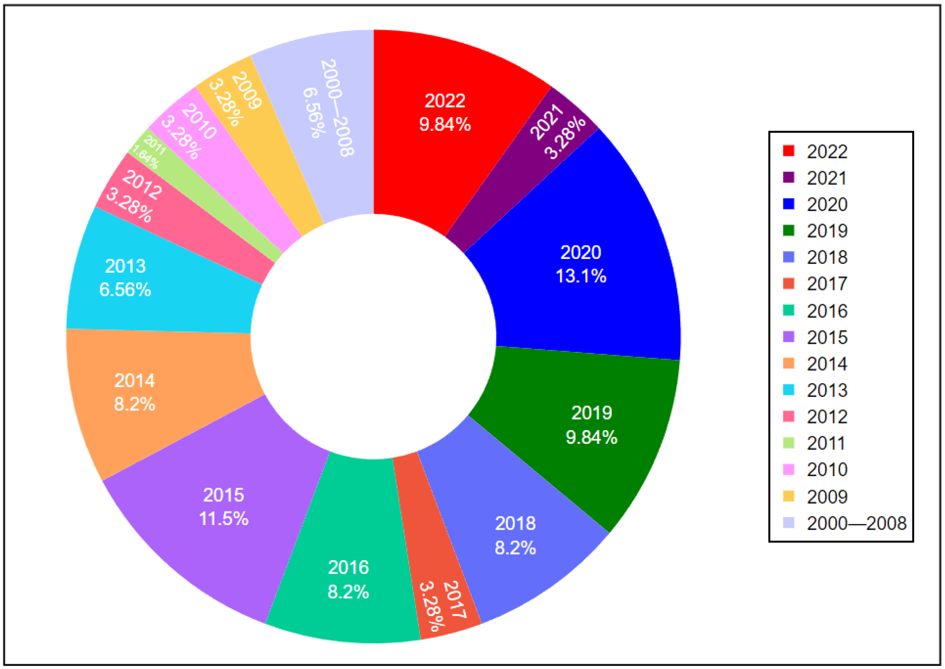
Figure 2.
Distribution of traffic models deployed in the reviewed studies in percentage.
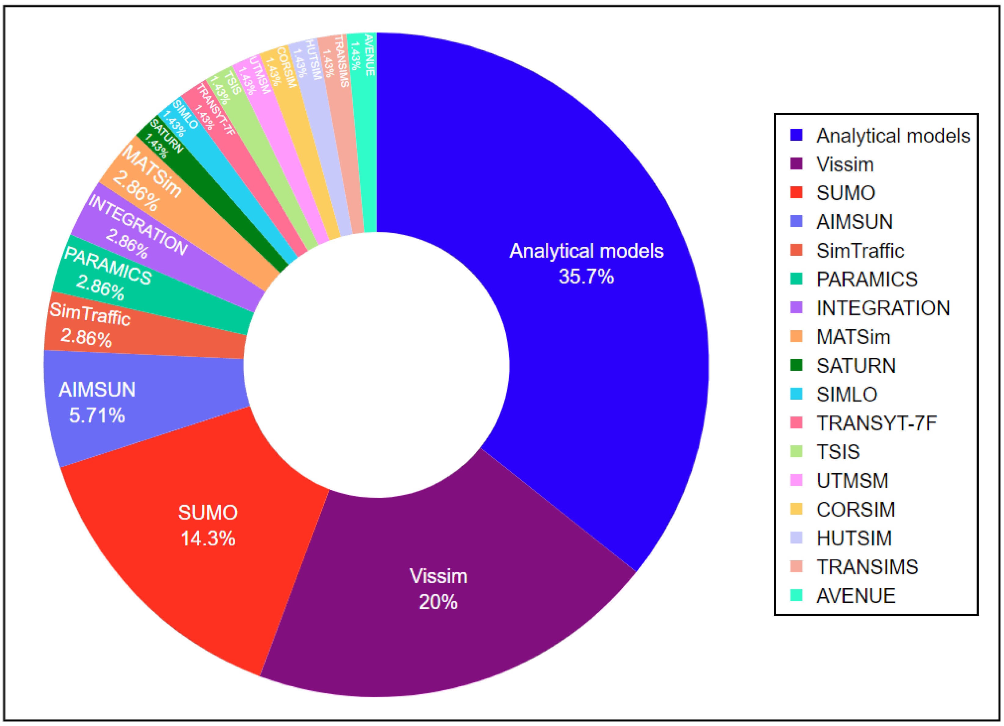
Figure 3.
Connections between studies, traffic programs, and fuel consumption/emissions models. Akçelik and Rouphail, 1993 [28], VISSIM [30], SUMO [31], AIMSUN [32], SATURN [36], Osorio and Bierlaire, 2009 [37], Chen et al., 2019b [38], Dong, 2016 [39], Treiber and Kesting, 2014 [40], OVM [41,42], SIMTraffic [43], PARAMICS [44], INTEGRATION [45], Cellular automata system [46], Wu and Li, 2009 [47], Yang, 2003 [48], HCM [29], MATSim [49], IDM [50], LWR [51], SIMLO [52], TRANSYT-7F [53,54], DynaTAIWAN [55], Webster, 1958 [12], CTM [56,57], TRANSIMS [58], TSIS [59], UTMSM [60], Akcelik, 1982 [61], CORSIM [62], Akçelik and Besley, 1984 [63], AVENUE [64], HUTSIM [65], Kovari et al., 2022 [66], Li et al., 2022 [67], Zhang et al., 2022 [68], Jovanović et al., 2022 [69], Ounoughi et al., 2022 [70], Abudayyeh et al., 2021 [71], Chen and Jia, 2021 [72], Lin et al., 2022 [73], Feng et al., 2020 [74], Bai et al., 2020 [75], Chen and Yuan, 2020 [76], Elidrissi et al., 2020 [77], Paul and Mitra, 2020 [78], Song et al., 2020 [79], Al-Turki et al., 2020 [80], Wu et al., 2020 [81], Calle-Laguna et al., 2019 [82], Chen et al., 2019a [83], Jia et al., 2019 [84], Li and Sun, 2019 [85], Wang et al., 2019 [86], Zheng et al., 2019 [87], Balta and Ozcelik, 2018 [88], Yao et al., 2018 [89], Kou et al., 2018 [90], Peres et al., 2018 [91], Shen, 2018 [92], Abdelghaffar et al., 2017 [93], Armas et al., 2017 [94], Ji et al., 2016 [95], Yu et al., 2016 [96], Haberl et al., 2016 [97], Han et al., 2016 [98], Tanaka, 2016 [99], Khalighi and Christofa, 2015 [100], Lin et al., 2015 [101], Olivera et al., 2015 [102], Osorio and Nanduri, 2015a [103], Osorio and Nanduri, 2015b [104], Li et al., 2015 [105], Stevanovic et al., 2015 [106], Dias et al., 2014 [107], Garcia-Nieto et al., 2014 [108], Ma et al., 2014 [109], Almasri, 2014 [110], Zhou and Cai, 2014 [111], Liao, 2013 [112], Lv et al., 2013 [113], Qian et al., 2013 [114], Zhang et al., 2013 [115], Kwak et al., 2012 [116], Zhang et al., 2012 [117], Li et al., 2011 [118], Zhang and Shang, 2010 [119], Ma and Nakamura, 2010 [120], Park et al., 2009 [121], Stevanovic et al., 2009 [122] Murat and Kikuchi, 2007 [123], Li et al., 2004 [124], Oda et al., 2004 [125], Niittyrnaki, 2001 [126], HBEFA in SUMO [35], VISSIM FC [30], Surrogate measure (Eco-PI) [127], SATURN FC [36], Panis, et al., 2006 [128], Jun and Pei, 2012 [129], Xiong et al., 2012 [130], Mayeres et al., 1996 [131], Liu, 2013 [132], Tang, 2013 [133], AIMSUN FC [32], Liao and Machemehl, 1998 [134], PARAMICS FC [44], VT-Micro [34], Li, 2001 [135], Elemental model [136], Sha, 2017 [137], Guo et al., 2012 [138], MOVES [139], Guo, 2014 [140], Tao, 2011 [141], CMEM [33], PHEM [142], Post et al., 1984 [143], Shabihkhani and Gonzales, 2013 [144], Xunan, 2014 [145], TRANSYT-7F FC [54], Elemental model [146], Wang et al., 2002 [147], Frey et al., 2001 [148], Frey et al., 2002 [149], TSIS FC [59], IVE [150], Zhang et al., 2009 [151], Oneyama et al., 2001 [152], SIDRA (Elemental model) [136,146,153], Li et al., 2003 [154], Oguchi et al., 2002 [155], HUTEMCA [65].
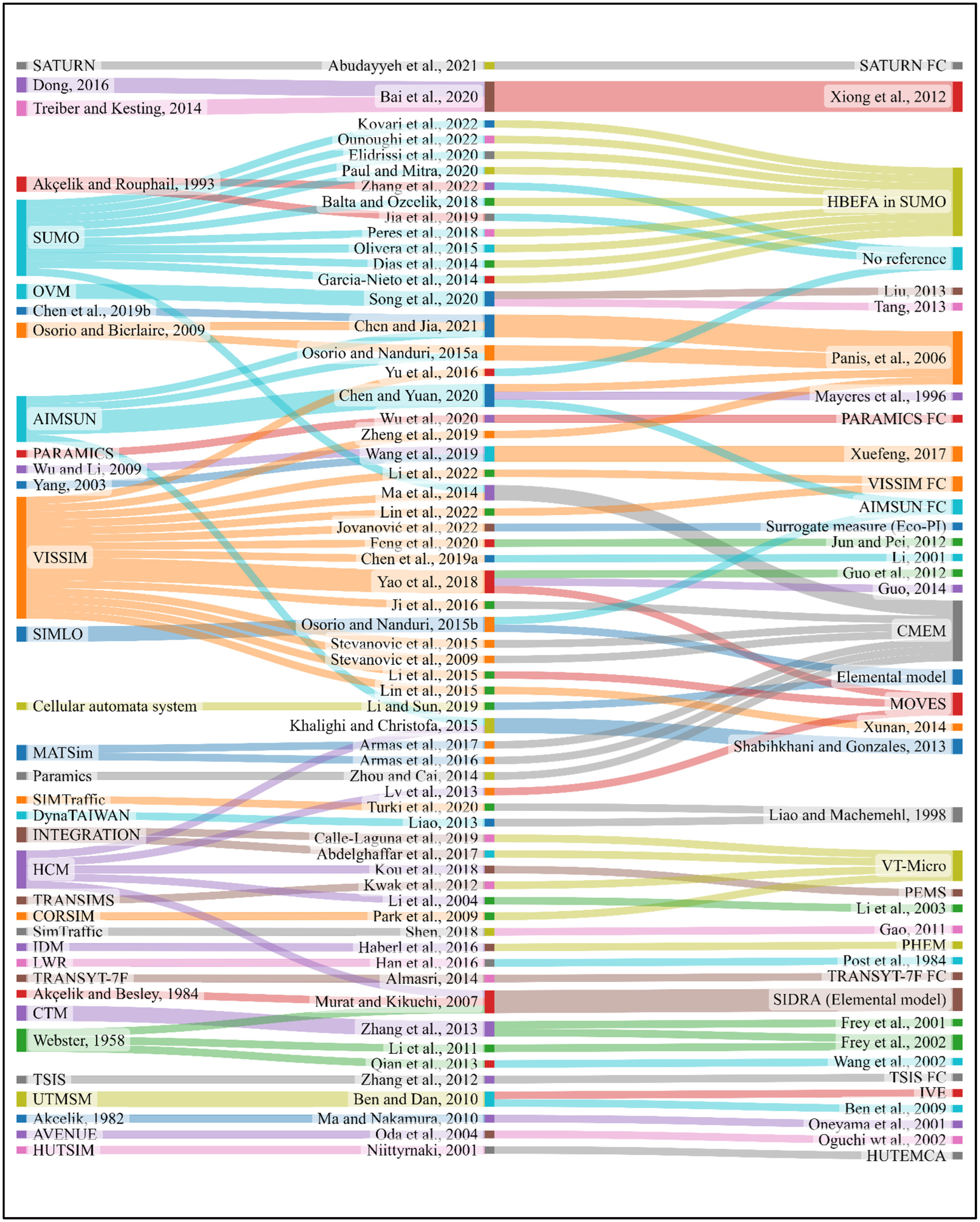
Figure 4.
Distribution of the fuel consumption and emissions models in percentage.
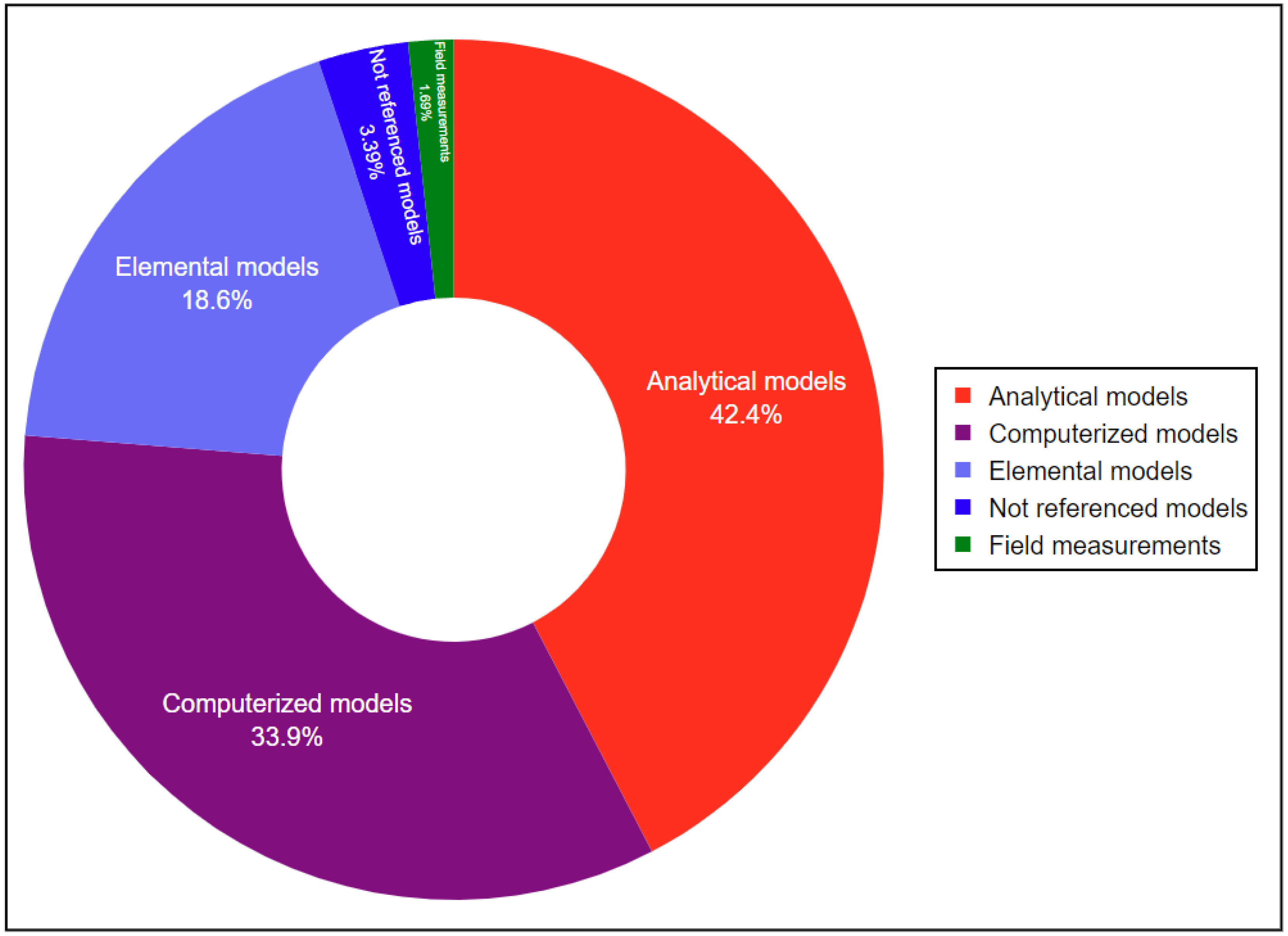
Figure 5.
Connections between studies, optimization techniques, and objective functions. Kovari et al., 2022 [66], Li et al., 2022 [67], Zhang et al., 2022 [68], Jovanović et al., 2022 [69], Ounoughi et al., 2022 [70], Abudayyeh et al., 2021 [71], Chen and Jia, 2021 [72], Lin et al., 2022 [73], Feng et al., 2020 [74], Bai et al., 2020 [75], Chen and Yuan, 2020 [76], Elidrissi et al., 2020 [77], Paul and Mitra, 2020 [78], Song et al., 2020 [79], Al-Turki et al., 2020 [80], Wu et al., 2020 [81], Calle-Laguna et al., 2019 [82], Chen et al., 2019a [83], Jia et al., 2019 [84], Li and Sun, 2019 [85], Wang et al., 2019 [86], Zheng et al., 2019 [87], Balta and Ozcelik, 2018 [88], Yao et al., 2018 [89], Kou et al., 2018 [90], Peres et al., 2018 [91], Shen, 2018 [92], Abdelghaffar et al., 2017 [93], Armas et al., 2017 [94], Ji et al., 2016 [95], Yu et al., 2016 [96], Haberl et al., 2016 [97], Han et al., 2016 [98], Tanaka, 2016 [99], Khalighi and Christofa, 2015 [100], Lin et al., 2015 [101], Olivera et al., 2015 [102], Osorio and Nanduri, 2015a [103], Osorio and Nanduri, 2015b [104], Li et al., 2015 [105], Stevanovic et al., 2015 [106], Dias et al., 2014 [107], Garcia-Nieto et al., 2014 [108], Ma et al., 2014 [109], Almasri, 2014 [110], Zhou and Cai, 2014 [111], Liao, 2013 [112], Lv et al., 2013 [113], Qian et al., 2013 [114], Zhang et al., 2013 [115], Kwak et al., 2012 [116], Zhang et al., 2012 [117], Li et al., 2011 [118], Zhang and Shang, 2010 [119], Ma and Nakamura, 2010 [120], Park et al., 2009 [121], Stevanovic et al., 2009 [122] Murat and Kikuchi, 2007 [123], Li et al., 2004 [124], Oda et al., 2004 [125], Niittyrnaki, 2001 [126].
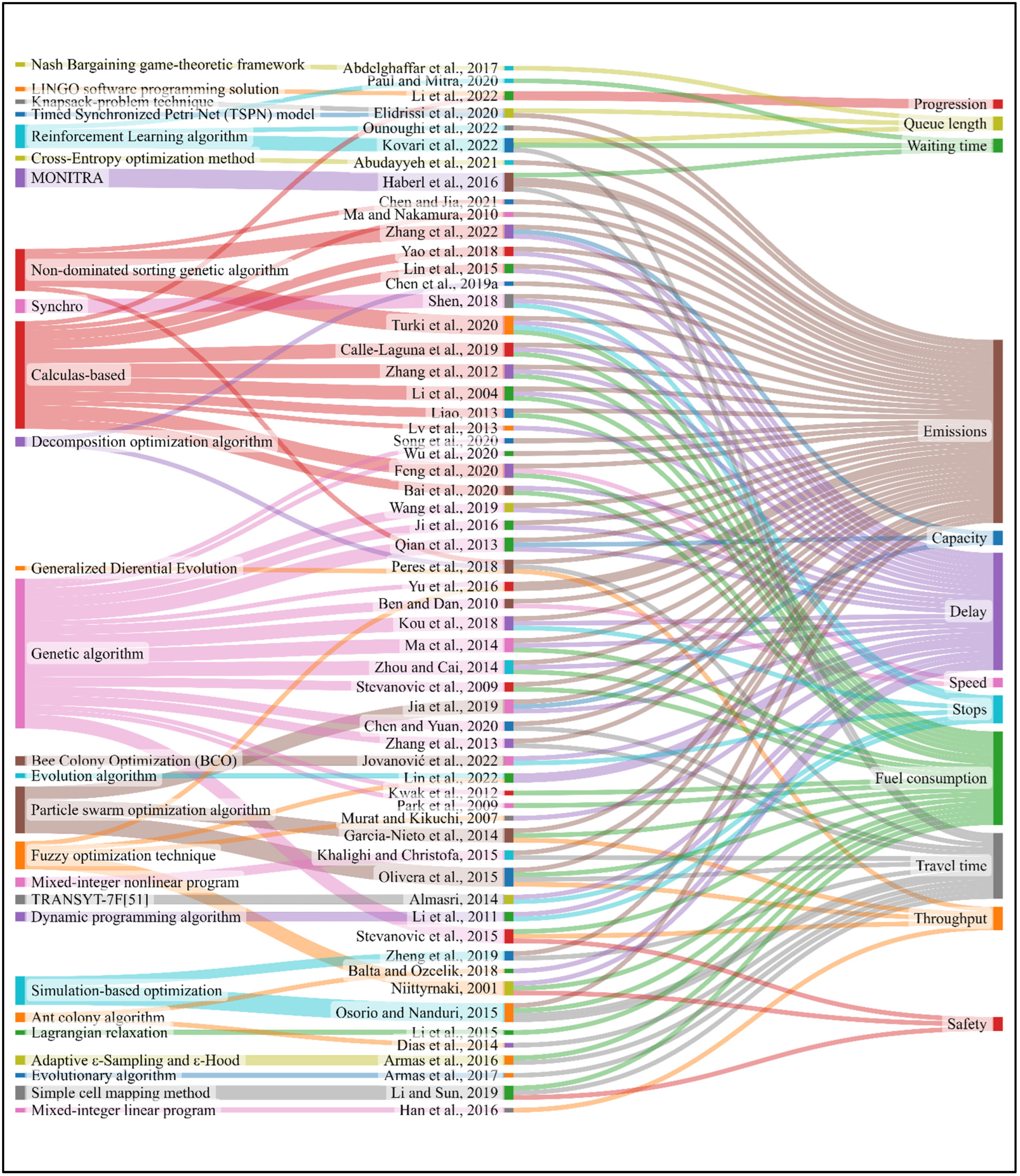

Table 1.
Data fidelity and factors used in the reviewed studies.
| Study | High-Resolution Data | Impactful Factors on Fuel Consumption and Emissions | |||
|---|---|---|---|---|---|
| Vehicle Type | Fleet Distribution | Grade | Cruising Speed | ||
| Kovari et al., 2022 [66] | ✓ | ✗ | ✗ | ✗ | ✓ |
| Li et al., 2022 [67] | ✓ | ✗ | ✗ | ✗ | ✓ |
| Zhang et al., 2022 [68] | ✗ | ✗ | ✗ | ✗ | ✓ |
| Jovanović et al., 2022 [69] | ✓ | ✓ | ✓ | ✗ | ✓ |
| Ounoughi et al., 2022 [70] | ✓ | ✗ | ✗ | ✗ | ✓ |
| Abudayyeh et al., 2021 [71] | ✗ | ✗ | ✗ | ✗ | ✓ |
| Chen and Jia, 2021 [72] | ✓ | ✗ | ✗ | ✗ | ✓ |
| Lin et al., 2021 [73] | ✓ | ✗ | ✗ | ✗ | ✓ |
| Feng et al., 2020 [74] | ✓ | ✗ | ✗ | ✗ | ✓ |
| Bai et al., 2020 [75] | ✗ | ✗ | ✗ | ✗ | ✓ |
| Chen and Yuan, 2020 [76] | ✓ | ✗ | ✗ | ✗ | ✓ |
| Elidrissi et al., 2020 [77] | ✓ | ✗ | ✗ | ✗ | ✓ |
| Paul and Mitra, 2020 [78] | ✓ | ✗ | ✗ | ✗ | ✓ |
| Song et al., 2020 [79] | ✗ | ✗ | ✗ | ✗ | ✓ |
| Al-Turki et al., 2020 [80] | ✗ | ✗ | ✗ | ✗ | ✓ |
| Wu et al., 2020 [81] | ✓ | ✗ | ✗ | ✗ | ✓ |
| Calle-Laguna et al., 2019 [82] | ✓ | ✗ | ✗ | ✗ | ✓ |
| Chen et al., 2019a [83] | ✓ | ✗ | ✗ | ✗ | ✓ |
| Jia et al., 2019 [84] | ✗ | ✗ | ✗ | ✗ | ✓ |
| Li and Sun, 2019 [85] | ✗ | ✗ | ✗ | ✗ | ✓ |
| Wang et al., 2019 [86] | ✗ | ✗ | ✗ | ✗ | ✓ |
| Zheng et al., 2019 [87] | ✓ | ✗ | ✗ | ✗ | ✓ |
| Balta and Ozcelik, 2018 [88] | ✓ | ✗ | ✗ | ✗ | ✓ |
| Yao et al., 2018 [89] | ✓ | ✗ | ✗ | ✗ | ✓ |
| Kou et al., 2018 [90] | ✗ | ✗ | ✗ | ✗ | ✓ |
| Peres et al., 2018 [91] | ✓ | ✗ | ✗ | ✗ | ✓ |
| Shen, 2018 [92] | ✗ | ✓ | ✗ | ✗ | ✓ |
| Abdelghaffar et al., 2017 [93] | ✓ | ✗ | ✗ | ✗ | ✓ |
| Armas et al., 2017 [94] | ✓ | ✓ | ✓ | ✗ | ✓ |
| Ji et al., 2016 [95] | ✓ | ✓ | ✓ | ✗ | ✓ |
| Yu et al., 2016 [96] | ✓ | ✓ | ✗ | ✗ | ✓ |
| Haberl et al., 2016 [97] | ✗ | ✗ | ✗ | ✗ | ✓ |
| Han et al., 2016 [98] | ✗ | ✗ | ✗ | ✗ | ✓ |
| Tanaka., 2016 [99] | ✓ | ✗ | ✗ | ✗ | ✓ |
| Khalighi and Christofa, 2015 [100] | ✗ | ✓ | ✓ | ✗ | ✓ |
| Lin et al., 2015 [101] | ✓ | ✗ | ✗ | ✗ | ✓ |
| Olivera et al., 2015 [102] | ✓ | ✗ | ✗ | ✗ | ✓ |
| Osorio and Nanduri, 2015a [103] | ✓ | ✓ | ✗ | ✗ | ✓ |
| Osorio and Nanduri, 2015b [104] | ✓ | ✗ | ✗ | ✗ | ✓ |
| Li et al., 2015 [105] | ✓ | ✗ | ✗ | ✗ | ✓ |
| Stevanovic et al., 2015 [106] | ✓ | ✓ | ✗ | ✗ | ✓ |
| Dias et al., 2014 [107] | ✓ | ✗ | ✗ | ✗ | ✓ |
| Garcia-Nieto et al., 2014 [108] | ✓ | ✗ | ✗ | ✗ | ✓ |
| Ma et al., 2014 [109] | ✓ | ✓ | ✓ | ✗ | ✓ |
| Almasri, 2014 [110] | ✗ | ✗ | ✗ | ✗ | ✓ |
| Zhou and Cai, 2014 [111] | ✓ | ✗ | ✗ | ✗ | ✓ |
| Liao, 2013 [112] | ✗ | ✗ | ✗ | ✗ | ✓ |
| Lv et al., 2013 [113] | ✗ | ✗ | ✗ | ✗ | ✓ |
| Qian et al., 2013 [114] | ✗ | ✗ | ✗ | ✗ | ✓ |
| Zhang et al., 2013 [115] | ✗ | ✗ | ✗ | ✗ | ✓ |
| Kwak et al., 2012 [116] | ✓ | ✗ | ✗ | ✗ | ✓ |
| Zhang et al., 2012 [117] | ✓ | ✗ | ✗ | ✗ | ✓ |
| Li et al., 2011 [118] | ✗ | ✗ | ✗ | ✗ | ✓ |
| Zhang and Shang, 2010 [119] | ✓ | ✗ | ✗ | ✗ | ✓ |
| Ma and Nakamura, 2010 [120] | ✗ | ✓ | ✓ | ✗ | ✓ |
| Park et al., 2009 [121] | ✓ | ✗ | ✗ | ✗ | ✓ |
| Stevanovic et al., 2009 [122] | ✓ | ✓ | ✗ | ✗ | ✓ |
| Murat and Kikuchi, 2007 [123] | ✗ | ✗ | ✗ | ✗ | ✓ |
| Li et al., 2004 [124] | ✗ | ✗ | ✗ | ✗ | ✓ |
| Oda et al., 2004 [125] | ✗ | ✗ | ✗ | ✗ | ✓ |
| Niittyrnaki, 2001 [126] | ✓ | ✗ | ✗ | ✗ | ✓ |
Table 2.
Saving (%) in sustainability metrics as documented by various studies.
| Study | Saving in Fuel Consumption and Vehicular Emissions | |||||
|---|---|---|---|---|---|---|
| FC | CO | CO2 | VOC (HC) | NOx | PM | |
| Kovari et al., 2022 [66] | - | - | 1.8 | - | - | - |
| Li et al., 2022 [67] | <18 | <18 | - | <18 | <18 | - |
| Zhang et al., 2022 [68] | - | 24.5–31.9 | - | - | - | - |
| Jovanović et al., 2022 [69] | - | - | - | - | - | - |
| Ounoughi et al., 2022 [70] | - | - | 30 | - | - | - |
| Abudayyeh et al., 2021 [71] | - | - | 8 | - | - | - |
| Chen and Jia, 2021 [72] | 8–9.8 | - | 1.9–2.9 | - | 4–5.6 | - |
| Lin et al., 2021 [73] | - | - | - | - | - | - |
| Feng et al., 2020 [74] | - | - | - | - | - | - |
| Bai et al., 2020 [75] | 26–29 | - | - | - | - | - |
| Chen and Yuan, 2020 [76] | - | - | <12 | 16–28 | <12 | 12.2 |
| Elidrissi et al., 2020 [77] | - | 40–51.4 | 16.6–30.7 | 37–48.3 | 13.5–33.7 | - |
| Paul and Mitra, 2020 [78] | 2.9–9.8 | - | 2.9–9.8 | - | - | - |
| Ze-Rui et al., 2020 [79] | - | - | - | - | - | - |
| Turki et al., 2020 [80] | 11.7–24.8 | 11.9–22.6 | - | - | 11.2–16.9 | - |
| Wu et al., 2020 [81] | - | 21.2–55.2 | - | 20–22.2 | 21.1–23.6 | - |
| Calle-Laguna et al., 2019 [82] | - | - | - | - | - | - |
| Chen et al., 2019a [83] | - | - | 31.3 | - | - | - |
| Jia et al., 2019 [84] | - | 3.2 | - | - | - | - |
| Li and Sun, 2019 [85] | 4–26.6 | - | - | - | - | - |
| Wang et al., 2019 [86] | - | <28 | - | <28 | - | - |
| Zheng et al., 2019 [87] | 1–32 | 1–32 | 1–32 | 1–32 | 1–32 | 1–32 |
| Balta and Ozcelik, 2018 [88] | 15–21 | - | 14–18 | - | - | - |
| Yao et al., 2018 [89] | - | 1.5–6.65 | - | 0.5–8.2 | 1–7.22 | - |
| Kou et al., 2018 [90] | - | <1 | 3.4–6 | 3.2–5.8 | 5.5–9.3 | 2.2–4.4 |
| Peres et al., 2018 [91] | - | 3.9–17.5 | 5.2–19.7 | 1–17.3 | 1.5–30.8 | 4.4–20.3 |
| Shen, 2018 [92] | - | 9.5–19.5 | - | 8.1–11.5 | 5.7–29.2 | - |
| Abdelghaffar et al., 2017 [93] | 6–13 | - | 6–13 | - | - | - |
| Armas et al., 2017 [94] | 6.1 | <1 | 7.5 | - | 2.9 | <1 |
| Ji et al., 2016 [95] | 4.4–27.6 | 3.6–25.1 | 1.6–25.6 | 4.2–34.5 | 6.7–31 | - |
| Yu et al., 2016 [96] | - | - | - | - | - | - |
| Haberl et al., 2016 [97] | - | 3.8–13.2 | 3.8–8.6 | - | 2.3–3.5 | 3.6–11.7 |
| Han et al., 2016 [98] | - | - | - | 2–2.1 | - | - |
| Tanaka., 2016 [99] | 9.4 | 1 | 10.3 | 3.4 | +4 | - |
| Khalighi and Christofa, 2015 [100] | - | - | - | 2.5–4.4 | 3.6–7.6 | - |
| Lin et al., 2015 [101] | - | 13.4 | - | 13.4 | 13.4 | - |
| Olivera et al., 2015 [102] | 6–18.2 | 23.3 | - | - | 29.3 | - |
| Osorio and Nanduri, 2015a [103] | - | - | 9.7 | 14.3 | 23.6 | - |
| Osorio and Nanduri, 2015b [104] | 1–30 | - | - | - | - | - |
| Li et al., 2015 [105] | 2 | - | - | - | - | - |
| Stevanovic et al., 2015 [106] | <4.5 | - | - | - | - | - |
| Dias et al., 2014 [107] | 1–49 | - | 1–49 | - | - | - |
| Garcia-Nieto et al., 2014 [108] | 12–43 | - | 12–43 | - | 12–43 | - |
| Ma et al., 2014 [109] | 2.4–5.34 | 14.6–15.6 | - | 13.5 | 7.4 | - |
| Almasri, 2014 [110] | 31 | - | - | - | - | - |
| Zhou and Cai, 2014 [111] | 5.8 | - | - | - | - | - |
| Liao, 2013 [112] | 2.2–40.9 | - | - | - | - | - |
| Lv et al., 2013 [113] | - | 2–11 | 2–11 | 2–11 | 2–11 | - |
| Qian et al., 2013 [114] | - | 5–30.5 | - | 5–30.7 | 5–30.6 | - |
| Zhang et al., 2013 [115] | - | 8 | - | - | - | - |
| Kwak et al., 2012 [116] | 20.3 | 7.8 | 20.5 | 15.3 | 20.6 | - |
| Zhang et al., 2012 [117] | 17 | 7 | - | - | - | - |
| Li et al., 2011 [118] | - | 7.3 | 26.4 | 27.8 | 12.3 | - |
| Zhang and Shang, 2010 [119] | - | 3.5 | - | - | - | - |
| Ma and Nakamura, 2010 [120] | - | - | - | - | 30.4 | - |
| Park et al., 2009 [121] | 5.5–8.7 | 3.5–17.5 | 5.8–8.3 | 3.7–14.1 | 4.9–16.3 | - |
| Stevanovic et al., 2009 [122] | 1–1.5 | - | 1.4 | - | - | - |
| Murat and Kikuchi, 2007 [123] | 1–11.1 | - | - | - | - | - |
| Li et al., 2004 [124] | - | 2.9 | - | 2.7 | 1.05 | - |
| Oda et al., 2004 [125] | - | - | 6.7 | - | - | - |
| Niittyrnaki, 2001 [126] | 26.6 | - | - | - | - | - |
Publisher’s Note: MDPI stays neutral with regard to jurisdictional claims in published maps and institutional affiliations. |
© 2022 by the authors. Licensee MDPI, Basel, Switzerland. This article is an open access article distributed under the terms and conditions of the Creative Commons Attribution (CC BY) license (https://creativecommons.org/licenses/by/4.0/).
Share and Cite
MDPI and ACS Style
Alshayeb, S.; Stevanovic, A.; Mitrovic, N.; Espino, E. Traffic Signal Optimization to Improve Sustainability: A Literature Review. Energies 2022, 15, 8452. https://doi.org/10.3390/en15228452
AMA Style
Alshayeb S, Stevanovic A, Mitrovic N, Espino E. Traffic Signal Optimization to Improve Sustainability: A Literature Review. Energies. 2022; 15(22):8452. https://doi.org/10.3390/en15228452
Chicago/Turabian StyleAlshayeb, Suhaib, Aleksandar Stevanovic, Nikola Mitrovic, and Elio Espino. 2022. "Traffic Signal Optimization to Improve Sustainability: A Literature Review" Energies 15, no. 22: 8452. https://doi.org/10.3390/en15228452
Note that from the first issue of 2016, this journal uses article numbers instead of page numbers. See further details here.