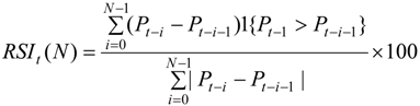
Article

Revisiting the Performance of MACD and RSI Oscillators

by
Terence Tai-Leung Chong
1,2,*,
Wing-Kam Ng
3 and
Venus Khim-Sen Liew
4
1
Hong Kong Institute of Asia-Pacific Studies, Department of Economics, The Chinese University of Hong Kong, Shatin, Hong Kong, China
2
Department of International Economics and Trade, Nanjing University, Nanjing, Jiangsu 210093, China
3
Department of Economics, The Chinese University of Hong Kong, Hong Kong, China
4
Faculty of Economics and Business, Universiti Malaysia Sarawak, Sarawak, Malaysia
*
Author to whom correspondence should be addressed.
J. Risk Financial Manag. 2014, 7(1), 1-12; https://doi.org/10.3390/jrfm7010001
Submission received: 25 October 2013 / Revised: 6 January 2014 / Accepted: 28 January 2014 / Published: 26 February 2014

Abstract

:
Chong and Ng (2008) find that the Moving Average Convergence–Divergence (MACD) and Relative Strength Index (RSI) rules can generate excess return in the London Stock Exchange. This paper revisits the performance of the two trading rules in the stock markets of five other OECD countries. It is found that the MACD(12,26,0) and RSI(21,50) rules consistently generate significant abnormal returns in the Milan Comit General and the S&P/TSX Composite Index. In addition, the RSI(14,30/70) rule is also profitable in the Dow Jones Industrials Index. The results shed some light on investors’ belief in these two technical indicators in different developed markets.

1. Introduction

Technical analysis has been widely applied in financial markets for decades. It examines how an investor may profit from the behavior observed in financial markets. Technical analysts believe that the historical performance of stock markets is an indication of future performance, and it is possible for one to develop profitable trading rules using historical prices, charts and related statistics. Conventional studies in technical trading rules, however, seldom provide explanations as to why these rules are profitable. Recently, behavioral finance, which studies how one can use psychology and other behavioral theories to explain the behavior of investors, has become the theoretical basis for technical analysis.
Whether technical trading rules can be relied upon to make investment decisions has been controversial. A considerable number of studies have investigated the performance of technical trading analysis. Jensen and Benington [1] indicate that past information cannot be used to predict future prices. Neftçi [2] argues that technical analysis cannot beat the market if the underlying process is linear. Allen and Karjalainen [3] also conclude that technical trading rules do not generate abnormal profits over the buy-and-hold strategy, especially after deducting transaction fees. More recently, Tanaka-Yamawaki and Tokuoka [4] also report that frequently used technical indicators, such as Moving Average Convergence–Divergence (MACD) and Relative Strength Index (RSI), are not effective in forecasting various selected intra-day US stock prices.
Treynor and Ferguson [5], however, argue that when the non-public information is considered, technical analysis can produce sizable profits. Bessembinder and Chan [6] conclude that the moving average and trading range breakout rules outperform the buy-and-hold strategy in Asian stock markets. Sullivan et al. [7], Gunasekarage and Power [8], Kwon and Kish [9] and Chong and Ng [10] also report significant excess returns to technical trading rules. Chong and Ip [11] show that the momentum strategy yields considerable returns in emerging currency markets. Lui and Chong [12] use the human trader experiment approach to compare the performance of experienced and novice traders. It is found that traders who are more knowledgeable on technical analysis significantly outperform those who are less knowledgeable.
In this paper, the profitability of the MACD and RSI, are evaluated. MACD was proven to be a valuable tool for traders in the 1980s, and RSI has also been popularly adopted since its introduction by Wilder in 1978 [13,14,15]. As of today, the two rules are still widely used as trading indicators in the market [16,17]. Despite their popularity and widespread use among traders and practitioners, they have been much neglected in the academic literature [18]1. As such, their empirical performance has yet to be formally analyzed. Notably, Chong and Ng [10] apply the MACD and RSI rules to 60-year monthly data (July 1935 to January 1994) of the London Stock Exchange FT30 Index. The authors conclude that MACD and RSI can generate significantly higher than the buy-and-hold strategy in this market. The current study extends that spirit of Chong and Ng [10] to investigate if such rules can generally generate excess returns for more markets other than the specific case of the London Stock Exchange. To this end, stock markets of five OECD countries are considered. Our results show that the MACD(12,26,0) and RSI(21,50) rules consistently generate significant abnormal returns in the Milan Comit General and the S&P/TSX Composite Index. This is probably because the Italian stock market is less developed compared to the stock markets of other major OECD countries and is therefore relatively inefficient. In addition, Section 2 briefly describes the data sets and the trading rules. Section 3 presents the empirical results, and Section 4 concludes our study.

2. Data and Methodology

The daily closing prices of the Milan Comit General, S&P/TSX Composite, DAX 30, Dow Jones Industrials and Nikkei 225 from January 1976 to December 2002 are obtained from DataStream.2 The profitability of the MACD and RSI trading rules for these indices will be evaluated. The MACD is constructed based on exponential moving averages. It is calculated by subtracting the longer exponential moving average (EMA) of window length N from the shorter EMA of window length M, where the EMA is computed as follows:
Jrfm 07 00001 i001
where EMAt(N) is the exponential moving average at time t, N is the window length of the EMA, and Pt is the value of index at time t. Two different MACD rules are examined:
Rule 1:
A buy signal is produced when MACD crosses zero from below, while a sell signal is obtained when MACD crosses zero from above. This trading rule is denoted as MACD(N, M, 0)3.
Rule 2:
A buy signal is generated when MACD crosses the nine-day EMA of the MACD from below, while a sell signal is obtained when MACD crosses the nine-day EMA of the MACD from above. This trading rule is denoted as MACD(N, M, 9).
For the RSI oscillator, it is computed as:
Jrfm 07 00001 i002
where RSIt(N) is the Relative Strength Index at time t, and N is the bandwidth. 1{·} is an indicator function, which equals one when the statement inside the bracket is true, and is zero otherwise. |x| is the absolute value of x. The values of the RSI range from 0 to 100 inclusively. A stock is considered as fairly priced if its RSI is at the centerline 50. Thus, whenever the RSI is above 50, it indicates a bullish market, while the market is considered to be bearish when the RSI is below 50. RSI may also be used to identify overbought (RSI > 70) and oversold (RSI < 30) markets. Two different RSI rules are studied in this paper:
Rule 3:
A buy signal is triggered when RSI crosses the centerline (RSI = 50) from below, while a sell signal is obtained when RSI crosses the centerline from above. This trading rule is denoted as RSI(N, 50). In this paper, the RSI(7, 50), RSI(14, 50) and RSI(21, 50) will be examined.
Rule 4:
The fourth rule utilizes the oversold and overbought zones. When RSI falls below oversold zone (RSI < 30) and rises above 30 again, a buy signal is obtained. A sell signal is produced when the RSI rises above the overbought zone (RSI > 70) and falls below 70 again. In this paper, we study RSI(14, 30/70) and RSI(21, 30/70).
We adopt the practice of Brock et al. [20] that whenever there is a buy or sell signal, all other signals in the next ten days are ignored. As such, the performance of MACD and RSI and the buy-and-hold return are evaluated on the basis of ten-day returns (rt10), which is computed as:
rt10 = log(Pt+10) − log(Pt)
where Pt is the closing price on day t4.
Table 1. Summary statistics for ten-day returns.
Milan Comit General76-02
Mean0.00390
S.D.0.04898
Skewness−0.26120 **
Kurtosis2.2802 **
S&P/TSX Composite Index76-02
Mean0.00282
S.D.0.03188
Skewness−0.93666 **
Kurtosis6.2533 **
DAX 3076-02
Mean0.00249
S.D.0.03883
Skewness−0.83329 **
Kurtosis4.7095 **
Dow Jones Industrials76-02
Mean0.00334
S.D.0.03218
Skewness−1.2985 **
Kurtosis12.375 **
Nikkei 225 Stock Average76-02
Mean0.00096
S.D.0.03656
Skewness−0.22022 **
Kurtosis2.5055 **
**: Indicates significance at the 5% level.

3. Empirical Results

3.1. Buy-and-Hold

The summary statistics for ten-day returns, which are also the returns of the buy-and-hold strategy, are reported in Table 1. The mean ten-day return of the five stock market indices ranges from 0.096% (Nikkei 225 Stock Average) to 0.39% (Milan Comit General). Note that the skewness of all the five series examined is significantly negative. Moreover, the ten-day returns for these indices are strongly leptokurtic, with the strongest kurtosis value documented for the Dow Jones Industrials. These findings are in line with those of the existing literature [8].

3.2. Trading Rules

The ten-day returns for our MACD and RSI trading rules are summarized in Table 2A to Table 3F. In these tables, “N(Buy)” and “N(Sell)” in the second and third columns respectively denote the number of buy-and-sell signals produced during the sample period. “Buy” and “Sell” in the next two columns in each table refer to the average ten-day returns generated by the corresponding buy-and-sell signals. Note that a negative return from the sell signal implies a positive profit. The t-statistics reported in these two columns test the null hypothesis of equality between the return generated by the trading rule (μr) and the buy-and-hold return (μ), i.e., Jrfm 07 00001 i003: μr = μ, where r denotes buy or sell. Following Brock et al. (1992), the 
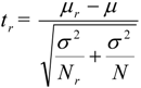
t-statistic for buy or sell returns is computed as:
Jrfm 07 00001 i004
where μ is the mean ten-day return of the sample, μr is the mean ten-day return of buy or sell signal, and Nr is the number of buy or sell signals. σ2 and 
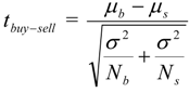
N are the estimated variances and the number of observations of the sample, respectively. “Buy > 0” and “Sell > 0” in the sixth and seventh columns refer to the fractions of times that the associated buy-and-sell signals are higher than zero. “Buy–Sell” in the last column contains the returns from buy signals less those from their sell signal counterparts. The null hypothesis of zero profit ( Jrfm 07 00001 i005=0) against the alternative of positive profit ( Jrfm 07 00001 i006 > 0) is tested using the following test statistic:
Jrfm 07 00001 i007
where μb and μs denote the mean ten-day returns of buy-and-sell signals, respectively, whereas Nb and Ns refer to the number of the corresponding buy-and-sell signals.
Rule 1
Table 2A summarizes the average ten-day return from the MACD(12,26,0) rule. The MACD(12,26,0) rule performs well in the Milan Comit General and the S&P/TSX Composite indices. The null hypothesis of the equality between returns from market indicators and the buy-and-hold strategy is rejected at conventional significance levels. This suggests that the trading strategy outperforms the buy-and-hold strategy. The most profitable buy (sell) signal appears in the Milan Comit General index with an average ten-day return of 1.379%. Note that the buy–sell returns are significantly positive. For the S&P/TSX Composite Index, both the null hypotheses are rejected at the 5% significance level.
Table 2A. Average ten-day returns from MACD(12,26,0).
Sample Period (76-02)N(Buy)N(Sell)BuySellBuy > 0Sell > 0Buy–Sell
Milan Comit General75790.01093−0.002860.6670.5060.01379 *
(1.236)(−1.220) (1.746)
S&P/TSX Composite Index72820.01159 **−0.001770.6940.5490.01335 **
(2.321)(−1.295) (2.593)
DAX 3078840.00404−0.000080.5640.4880.00411
(0.350)(−0.602) (0.674)
Dow Jones Industrials931040.004640.005340.6240.615−0.00070
(0.386)(0.628) (−0.152)
Nikkei 225 Stock Average78880.004570.004850.5510.602−0.00029
(0.866)(0.992) (−0.050)
**: Indicates significance at the 5% level;*: Indicates significance at the 10% level.
Rule 2
Table 2B shows the results of the MACD(12,26,9) rule. For Germany, the performance of this rule is far from satisfactory. The rule is unable to yield a higher profit than the buy-and-hold strategy. The buy–sell return is significantly negative at the 5% level, suggesting that investors who follow the trading signals of MACD(12,26,9) will suffer a negative return of 0.944% from a pair of buy-and-sell signals. The loss is sizeable compared to the positive buy-and-hold return of 0.249%.
Table 2B. Average ten-day returns from MACD(12,26,9).
Sample Period (76-02)N(Buy)N(Sell)BuySellBuy > 0Sell > 0Buy–Sell
Milan Comit General1571640.003670.003070.5290.5610.00060
(−0.058)(−0.215) (0.110)
S&P/TSX Composite Index1611620.002540.002430.5220.5190.00011
(−0.111)(−0.155) (0.031)
DAX 30168182−0.002010.00743 *0.5240.593−0.00944 **
(−1.484)(1.693) (−2.272)
Dow Jones Industrials178167−0.000060.004360.5450.527−0.00442
(−1.390)(0.405) (−1.274)
Nikkei 225 Stock Average1751540.00078−0.000880.5660.5130.00166
(−0.064)(−0.616) (0.410)
**: Indicates significance at the 5% level; *: Indicates significance at the 10% level.
Among the five series examined, the trading rules perform the worst in the DAX 30. For the remaining series, the 
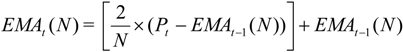
MACD(12,26,9) has no predictability. As the combination of eight-day, seventeen-day EMAs and signal line crossover can produce more reliable buy signals [21], we also examine the MACD(8,17,9) rule in this paper. From Table 2C, the return from buy signals is negative for Italy. For Germany, the MACD(8,17,9) rule produces sell signals which yield negative returns. The buy–sell returns are also significantly negative at the 5% level for both countries.
Table 2C. Average ten-day returns from MACD(8,17,9).
Sample Period (76-02)N(Buy)N(Sell)BuySellBuy > 0Sell > 0Buy–Sell
Milan Comit General194185−0.00272 *0.007380.4480.589−0.01010 **
(−1.857)(0.953) (−2.007)
S&P/TSX Composite Index1861970.004240.001580.5750.5180.00266
(0.599)(−0.539) (0.816)
DAX 30201190−0.001430.00755 *0.5120.621−0.00898 **
(−1.412)(1.770) (−2.286)
Dow Jones Industrials2051940.002420.002940.5660.593−0.00051
(−0.402)(−0.172) (−0.160)
Nikkei 225 Stock Average195193−0.000690.000220.5130.523−0.00090
(−0.620)(−0.278) (−0.244)
**: Indicates significance at the 5% level.
Rule 3
From Table 3A, the RSI(7,50) rule generates negative returns in the Milan Comit General. The results in Table 3B indicate that the 14-day RSI rule has some predictability too. In general, the buy–sell values are positive, implying that the rule is profitable. In most cases, the RSI(14,50) rule is able to generate profits. The predictability of the trading rule for the 21-day RSI is reported in Table 3C. The rule beats the buy-and-hold strategy in the Milan Comit General and the S&P/TSX Composite.
Table 3A. Average ten-day returns from RSI(7, 50).
Sample Period (76-02)N(Buy)N(Sell)BuySellBuy > 0Sell > 0Buy–Sell
Milan Comit General188199−0.00215 *0.006680.4630.558−0.00884 *
(−1.671)(0.791) (−1.774)
S&P/TSX Composite Index1712160.002320.001750.5260.5280.00057
(−0.203)(−0.488) (0.176)
DAX 301682240.001230.006630.5600.589−0.00541
(−0.416)(1.571) (−1.364)
Dow Jones Industrials1762310.003120.000280.5800.5280.00284
(−0.089)(−1.422) (0.882)
Nikkei 225 Stock Average182205−0.000660.001350.5490.556−0.00201
(−0.591)(0.151) (−0.541)
*: Indicates significance at the 10% level.
Table 3B. Average ten-day returns from RSI(14, 50).
Sample Period (76-02)N(Buy)N(Sell)BuySellBuy > 0Sell > 0Buy–Sell
Milan Comit General1361290.00433−0.00488**0.5150.4420.00921
(0.102)(−2.017) (1.530)
S&P/TSX Composite Index1281500.003720.000690.5390.50.00303
(0.318)(−0.809) (0.791)
DAX 301421650.004270.000820.5420.5270.00345
(0.540)(−0.546) (0.776)
Dow Jones Industrials1451740.004920.003180.6070.50.00174
(0.585)(−0.064) (0.481)
Nikkei 225 Stock Average1441630.00430−0.000310.5970.5030.00461
(1.084)(−0.439) (1.103)
**: Indicates significance at the 5% level.
Table 3C. Average ten-day returns from RSI(21, 50).
Sample Period (76-02)N(Buy)N(Sell)BuySellBuy > 0Sell > 0Buy–Sell
Milan Comit General1111040.01200 *−0.01069 **0.6130.4040.02268 **
(1.728)(−3.014) (3.394)
S&P/TSX Composite Index1191110.00614−0.00271 *0.5460.4500.00885 *
(1.127)(−1.813) (2.105)
DAX 301181260.004550.001780.5760.5240.00278
(0.572)(−0.204) (0.558)
Dow Jones Industrials1191460.002870.001530.5970.5410.00134
(−0.160)(−0.674) (0.337)
Nikkei 225 Stock Average1221210.00016−0.000550.5250.4790.00071
(−0.239)(−0.449) (0.151)
**: Indicates significance at the 5% level;*: indicates significance at the 10% level.
Table 3D. Average ten-day returns from RSI(7, 30/70).
Sample Period (76-02)N(Buy)N(Sell)BuySellBuy > 0Sell > 0Buy–Sell
Milan Comit General189211−0.00504 **0.006590.4440.545−0.01163 **
(−2.475)(0.786) (−2.371)
S&P/TSX Composite Index1772320.001790.005610.4970.569−0.00382
(−0.425)(1.311) (−1.201)
DAX 301872430.002260.002680.5400.527−0.00042
(−0.081)(0.076) (−0.112)
Dow Jones Industrials1922390.005740.002170.5570.5520.00357
(1.018)(−0.552) (1.143)
Nikkei 225 Stock Average187229−0.003390.002100.5130.559−0.00549
(−1.604)(0.464) (−1.523)
**: Indicates significance at the 5% level.
Table 3E. Average ten-day returns from RSI(14, 30/70).
Sample period (76-02)N(Buy)N(Sell)BuySellBuy > 0Sell > 0Buy–Sell
Milan Comit General132158−0.002420.007830.4920.614−0.01025 *
(−1.468)(0.997) (−1.774)
S&P/TSX Composite Index1271690.005690.001750.6140.5330.00393
(1.003)(−0.429) (1.050)
DAX 301141670.001350.01049 **0.4910.653−0.00914 *
(−0.312)(2.628) (−1.937)
Dow Jones Industrials1111640.01017 **0.003670.6580.5850.00650
(2.217)(0.128) (1.643)
Nikkei 225 Stock Average125164−0.00114−0.000310.4960.518−0.00083
(−0.636)(−0.440) (−0.191)
**: Indicates significance at the 5% level; *: Indicates significance at the 10% level.
Table 3F. Average ten-day returns from RSI(21, 30/70).
Sample period (76-02)N(Buy)N(Sell)BuySellBuy > 0Sell > 0Buy–Sell
Milan Comit General93127−0.00842 **0.004240.3980.559−0.01266*
(−2.410)(0.077) (−1.894)
S&P/TSX Composite Index741270.00074−0.000760.5410.5200.00150
(−0.558)(−1.254) (0.322)
DAX 3066113−0.004150.004090.4700.584−0.00824
(−1.383)(0.435) (−1.370)
Dow Jones Industrials601100.000850.003860.50.609−0.00301
(−0.598)(0.166) (−0.583)
Nikkei 225 Stock Average70118−0.003660.003510.5140.559−0.00717
(−1.052)(0.752) (−1.301)
**: Indicates significance at the 5% level; *: Indicates significance at the 10% level.
Rule 4
From Table 3D, most series have negative returns under the RSI(7, 30/70) rule. The return in Milan Comit General is significantly negative. The loss is 1.163% from a pair of buy-and-sell transactions. For other countries, none of the returns is significantly higher than the buy-and-hold strategy. The RSI(14, 30/70) rule yields negative returns for three series. For the Milan Comit General, a pair of buy-and-sell transactions generate a negative return of 1.03%, while it is −0.91% for the DAX30. Note that the sell signal produces a significant loss of 1.049% for the DAX30. However, the rule slightly outperforms the buy-and-hold strategy in the Dow Jones Industrials. For all other rules, no significant return is found. The RSI(21, 30/70) rule generates a negative return for the Milan Comit General.

3.3. Transaction Cost

The above results are obtained in the absence of transaction costs. In this section, we relax this assumption. According to the survey of Hudson et al. [22] on stockbrokers and stock broking divisions of major clearing banks, the minimum commission fee is at least 0.1%. When the bid-offer spreads of 0.5% and government stamp duty of 0.5% are included, the round-trip transaction cost is at least 1%.5 They show that technical trading rules of Brock et al. [20] do not generate excess returns in the UK market after taking a round-trip transaction cost of 1% into consideration. Mills [23] also shows that the moving average and trading range breakout rules cannot produce returns higher than the buy-and-hold strategy when a 1% transaction cost is taken into account. Therefore, in this paper, a 1% transaction cost is included to compute the net profits from each of the trading rule.6 We will focus on the Italian and Canadian markets, which contain the largest number of profitable trading rules. It is found that in the presence of a 1% transaction cost, the MACD(12,26,0) applied to these two countries are still profitable. For the Milan Comit General Index and S&P/TSX Composite Index, the net profits of the MACD(12,26,0) rule are 1.021%7 and 0.776% respectively. Moreover, the average annual return of the RSI(21,50) rule net of a 1% round-trip transaction cost for the Milan Comit General Index is 5.069%.

4. Conclusions

The discipline of finance has been dominated by the Efficient Market Hypothesis (EMH) for four decades since the pioneering work of Fama [25]. However, the EMH is built upon the assumption that investors are rational and fully informed. If technical analysis can yield abnormal returns, it implies that the EMH and its underlying assumptions fail to hold. In recent years, researchers have attempted to identify profitable trading rules resulting from patterns of human behavior. This study contributes to the existing literature of behavioral finance by reporting the profitability of two oscillators, namely the Moving Average Convergence–Divergence (MACD) and Relative Strength Index (RSI) in five major OECD markets. The two rules have been widely used by investors, but their empirical performance is relatively unexplored.
This study finds that the centerline crossover of the RSI has predictive ability in the Italian and Canadian stock markets. In particular, the RSI(21,50) rule performs well in the Milan Comit General Index. The RSI(14,30/70) rule is also profitable in the Dow Jones Industrials Index. The profits are sustainable in the presence of a 1% round-trip transaction cost. These findings are in line with Chong and Ng [10] that the MACD and RSI rules can generate significant profit for FT30. However, for the Nikkei 225 Stock Average, none of the rules can beat the buy-and-hold strategy. When the two rules of RSI are compared, it is found that the performance of centerline crossover is better. Our results shed some light on investors’ belief in these two technical indicators in different developed markets. The presence of trading rule profits also indicates that investors in these markets may only be boundedly rational.
Notably, Chong and Ng [10] demonstrate that MACD and RSI rules are robust to the choice of sample. However, it is important to note that the current study finds that these rules are not robust to the choice of market. Taking these findings together, before adopting these rules, it is advisable for traders and practitioners to at least ascertain the profitability of these rules in their markets using historical data. In addition, a simulation trading portfolio could be created in order to discover the full potential of these indicators under a real situation.8 Moreover, practitioners or academics may examine the profitability of these rules for individual shares as an extension in the spirit of this study.

References not cited

  1. M.C. Jensen, and G.A. Benington. “Random walk and technical theories: Some additional evidence.” J. Financ. 25 (1970): 469–482. [Google Scholar] [CrossRef]
  2. S.N. Neftçi. “Naïve trading rules in financial markets and Wiener-Kolmogorov prediction theory: A study of “technical analysis”.” J. Bus. 64 (1991): 549–571. [Google Scholar]
  3. F. Allen, and R. Karjalainen. “Using genetic algorithms to find technical trading rules.” J. Financ. Econ. 51 (1999): 245–271. [Google Scholar] [CrossRef]
  4. M. Tanaka-Yamawaki, and S. Tokuoka. “Adaptive use of technical indicators for the prediction of intra-day stock prices.” Phys. A 383 (2007): 125–133. [Google Scholar] [CrossRef]
  5. J.L. Treynor, and R. Ferguson. “In defense of technical analysis.” J. Financ. 40 (1985): 757–773. [Google Scholar] [CrossRef]
  6. H. Bessembinder, and K. Chan. “The profitability of technical rules in the Asian stock markets.” Pac. Basin Financ. J. 3 (1995): 257–284. [Google Scholar] [CrossRef]
  7. R. Sullivan, A. Timmerman, and H. White. “Data-snooping, technical trading rule performance and the Bootstrap.” J. Financ. 54 (1999): 1647–1691. [Google Scholar] [CrossRef]
  8. A. Gunasekarage, and D.M. Power. “The profitability of moving average trading rules in South Asian stock markets.” Emerg. Mark. Rev. 2 (2001): 17–33. [Google Scholar] [CrossRef]
  9. K.Y. Kwon, and R.J. Kish. “Technical trading strategies and return predictability: NYSE.” Appl. Financ. Econ. 12 (2002): 639–653. [Google Scholar] [CrossRef]
  10. T.T.-L. Chong, and W.K. Ng. “Technical analysis and the London stock exchange: Testing the MACD and RSI rules using the FT30.” Appl. Econ. Lett. 15 (2008): 1111–1114. [Google Scholar] [CrossRef]
  11. T.T.-L. Chong, and H. Ip. “Do momentum-based strategies work in emerging currency markets? ” Pac. Basin Financ. J. 17 (2009): 479–493. [Google Scholar] [CrossRef]
  12. K.M. Lui, and T.T.-L. Chong. “Do technical analysts outperform novice traders: Experimental evidence.” Econ. Bull. 33 (2013): 3080–3087. [Google Scholar]
  13. J.W. Wilder. New Concepts in Technical Trading Systems. Greensboro, NC, USA: Trend Research, 1978. [Google Scholar]
  14. S.P. Stawicki. “Application of financial analysis techniques to vital sign data: A novel method of trend interpretation in the intensive care unit.” OPUS12 Sci. 1 (2007): 14–16. [Google Scholar]
  15. H. Ni, and H. Yin. “Exchange rate prediction using hybrid neural networks and trading indicators.” Neurocomputing 72 (2009): 2815–2823. [Google Scholar] [CrossRef]
  16. R. White. “Technical Analysis Indicator That Works Turns Positive For These Stocks.” Forbes. 15 April 2013. Available online: http://www.forbes.com/sites/greatspeculations/2013/04/15/technical-analysis-indicator-that-works-turns-positive-for-these-stocks/ (accessed on 27 December 2013).
  17. R. Rosillo, D. de la Fuente, and J.A.L. Brugos. “Technical analysis and the Spanish stock exchange: Testing the RSI, MACD, momentum and stochastic rules using Spanish market companies.” Appl. Econ. 45 (2013): 1541–1550. [Google Scholar] [CrossRef]
  18. N. Ülkü, and E. Prodan. “Drivers of technical trend-following rules’ profitability in world stock markets.” Int. Rev. Financ. Anal. 30 (2013): 214–229. [Google Scholar] [CrossRef]
  19. J.J. Murphy. Technical Analysis of the Financial Markets: A Comprehensive Guide to Trading Methods and Applications. New York, NY, USA: New York Institute of Finance, 1999. [Google Scholar]
  20. W. Brock, J. Lakonishok, and B. LeBaron. “Simple technical trading rules and the stochastic properties of stock returns.” J. Financ. 5 (1992): 1731–1764. [Google Scholar]
  21. M.J. Pring. Momentum Explained. New York, NY, USA: McGraw-Hill, 2002, Volume 1 & 2. [Google Scholar]
  22. R. Hudson, M. Dempsey, and K. Keasey. “A note on the weak form efficiency of capital markets: The application of simple technical trading rules to UK stock prices—1935 to 1994.” J. Bank. Financ. 20 (1996): 1121–1132. [Google Scholar] [CrossRef]
  23. T.C. Mills. “Technical analysis and the London Stock Exchange: Testing trading rules using the FT30.” Int. J. Financ. Econ. 2 (1997): 319–331. [Google Scholar] [CrossRef]
  24. K.G. Rouwenhorst. “International momentum strategies.” J. Financ. 53 (1998): 267–284. [Google Scholar] [CrossRef]
  25. E.F. Fama. “Efficient capital market, a review of theory and empirical work.” J. Financ. 25 (1970): 383–417. [Google Scholar] [CrossRef]
  • 1See [18], among the few for a recent application of these technical indicators in the Spanish stock market.
  • 2In examining the predictability of MACD and RSI rules in different sub-samples, Chong and Ng [6] demonstrate that these rules are robust to the choice of sample period.
  • 3The MACD(12,26,0) is the most commonly used MACD [14].
  • 4A negative return from the sell signal implies a positive profit.
  • 5Due to the increasing competition among stock brokers and the introduction of internet trading, transaction costs have been reduced sharply in recent years. It is expected that the trend of this reduction in transaction cost will continue, which will provide more room for the development of technical trading rules in the future.
  • 6Rouwenhorst [19] points out that for the large and liquid stock markets in Europe, the transaction cost is less than 1%.
  • 7Note that there are 75 buy signals and 79 sell signals over the 27-year period. Therefore, the annual return net of transaction cost is (1.093% − 0.5%) × 75/27 + (0.286% − 0.5%) × 79/27 = 1.021%.
  • 8We thank an anonymous referee for giving us this suggestion.

