Validation of the Merton Distance to the Default Model under Ambiguity

Abstract
:1. Introduction
2. Models
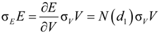
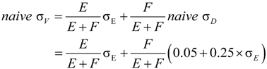
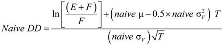
2.1. Naive Merton DD Model

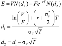
2.2. Merton’s DD Model under Ambiguity
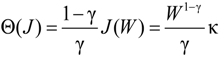
 and that the value function takes the form:
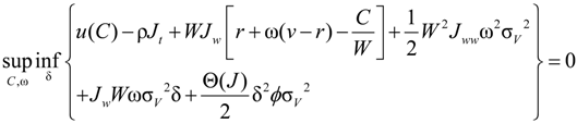
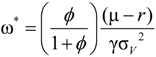
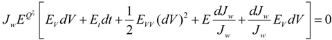
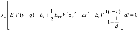
 . After taking derivatives of Equation (11) with respect to ω and some computation, we obtain the optimal investment in the firm for the ambiguity-averse investor:

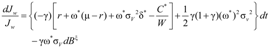
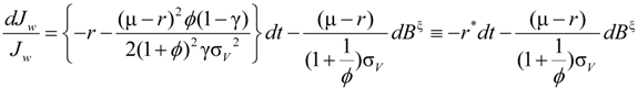
 , the dynamic process of the investor’s marginal utility function can be shown to be:
 .
.
 and
and  .
.
 ,
,  .
.2.3. Default Probability under Ambiguity
 , where
  and
and  . We can see that the default probability of the fixed income, debt, is modified due to investors’ ambiguity aversion. Similarly, the actual probability that a firm will default is computed as π = N(−d2), where
  and
and  .
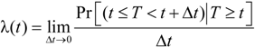
. , where
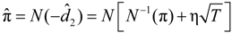
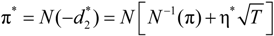
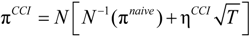
  is the risk-neutral default probability, and π = N(−d2) is the actual default probability (refer to [28,29,30] for more information of survival analysis). As the default probability under ambiguity is difficult to explore, we applied this approach to imply the default probability under ambiguity from the actual default probability, as follows. The mapping between the two default probabilities is:
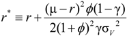
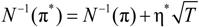 , we find that
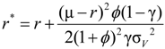
 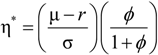 , where φ is the penalty parameter, used to depict the investor’s confidence about the reference model.
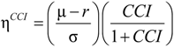
2.4. Cox Proportional Hazard Model

2.5. Credit Default Swap Spread Regression
3. Data

| Variable | Quantiles | ||||||
|---|---|---|---|---|---|---|---|
| Mean | SD | Min | 0.25 | Median | 0.75 | Max | |
| E | 59,213.18 | 74,361.40 | 0.45 | 13,575.92 | 28,167.40 | 74,009.42 | 519,044.42 |
| F | 41,562.61 | 57,808.95 | 684.97 | 17,509.28 | 23,839.00 | 38,574.00 | 761,203.00 |
| r (%) | 2.29 | 2.00 | −0.02 | 0.21 | 1.72 | 4.04 | 6.39 |
| CCI | 86.94 | 28.22 | 25.30 | 61.40 | 92.95 | 106.13 | 144.70 |
| r spread (%) | 0.77 | 10.45 | −69.01 | −4.58 | 0.80 | 6.48 | 89.40 |
| 1/σE | 1.91 | 0.44 | 0.52 | 1.58 | 1.92 | 2.24 | 3.13 |
| naive σv (%) | 37.00 | 10.03 | 17.92 | 29.84 | 35.38 | 42.43 | 76.44 |
| πnaive (%) | 6.43 | 9.53 | 0.00 | 0.23 | 2.58 | 8.20 | 54.21 |
| πCCI (%) | 6.59 | 9.36 | 0.00 | 0.33 | 2.81 | 8.59 | 53.56 |
| Corr(πnaive, πCCI) = 0.994 |
4. Empirical Results
4.1. Hazard Model Results
| Dependent Variable: Time to default | ||||||
|---|---|---|---|---|---|---|
| Variable | Model 1 | Model 2 | Model 3 | Model 4 | Model 5 | Model 6 |
| πnaive | −0.183 * | 0.733 * (0.062) | 0.504 * | |||
| (0.018) | (0.077) | |||||
| πCCI | −21.065 * | −97.848 * | −22.196 * | −76.093 * | ||
| (1.981) | (7.726) | (1.879) | (9.071) | |||
| CCI | 0.021 * | 0.015 * | 0.013 * | |||
| (0.002) | (0.002) | (0.002) | ||||
| ln(E) | −0.758 * | −0.721 * | −0.698 * | |||
| (0.035) | (0.035) | (0.035) | ||||
| ln(F) | 0.746 * | 0.938 * | 0.920 * | |||
| (0.048) | (0.052) | (0.051) | ||||
| 1/σE | −2.208 * | −2.170 * | −2.177 * | |||
| (0.168) | (0.167) | (0.164) | ||||
| r spread | 0.814 | −3.800 * | −3.783 * | |||
| (0.342) | (0.636) | (0.638) | ||||
| Variable | Quantiles | ||||||
|---|---|---|---|---|---|---|---|
| Mean | SD | Min | 0.25 | Median | 0.75 | Max | |
| CDS spread | 134.01 | 405.39 | 10.00 | 43.28 | 61.00 | 102.50 | 10,255.00 |
| πnaive | 5.07 | 11.86 | 0.00 | 0.00 | 0.03 | 2.77 | 68.63 |
| πCCI | 5.02 | 11.79 | 0.00 | 0.00 | 0.02 | 2.59 | 68.59 |
| Variable | Dependent variable: log(CDS spread) | ||
|---|---|---|---|
| Model 1 | Model 2 | Model 3 | |
| Constant | −1.8494 * (0.0011) | −1.6551 * (0.0169) | −1.3999 * (0.0776) |
| log(πnaive) | 0.1478 * (0.0050) | −0.2025 * (0.0599) | |
| log(πCCI) | 0.1735 * (0.0058) | 0.4075 * (0.0695) | |
| Obs. | 2107 | 2107 | 2107 |
| R2 | 0.2919 | 0.2995 | 0.3033 |
4.2. CDS Spread Regressions
5. Conclusions
Acknowledgments
Author Contributions
Conflicts of Interest
References
- R.C. Merton. “On the Pricing of Corporate Debt: The Risk Structure of Interest Rates.” J. Financ. 29 (1974): 449–470. [Google Scholar]
- J.Y. Campbell, J. Hilscher, and J. Szilagyi. “In Search of Distress Risk.” J. Financ. 63 (2008): 2899–2939. [Google Scholar] [CrossRef]
- S. Bharath, and T. Shumay. “Forecasting Default with the Merton Distance to Default Model.” Rev. Financ. Stud. 21 (2008): 1339–1369. [Google Scholar] [CrossRef]
- P. Crosbie, and J. Bohn. “Modeling Default Risk.” 2003. Available online: http://business.illinois.edu/gpennacc/MoodysKMV.pdf (accessed on 20 March 2014).
- M. Vassalou, and Y. Xing. “Default Risk in Equity Returns.” J. Financ. 59 (2004): 831–868. [Google Scholar] [CrossRef]
- D. Ellsberg. “Risk, Ambiguity, and Savage Axioms.” J. Econ. 75 (1961): 643–669. [Google Scholar]
- T.F. Bewley. “Knightian Decision Theory and Econometric Inferences.” J. Econ. Theor. 146 (2011): 1134–1147. [Google Scholar] [CrossRef]
- J. Dow, and S. R. Werlang. “Uncertainty Aversion, Risk Aversion and the Optimal Choice of Portfolio.” Econometrica 60 (1992): 197–204. [Google Scholar] [CrossRef]
- L. Epstein, and T. Wang. “Intertemporal Asset Pricing under Knightian Uncertainty.” Econometrica 62 (1994): 283–322. [Google Scholar] [CrossRef]
- Z. Chen, and L. Epstein. “Ambiguity, Risk and Asset Returns in Continuous Time.” Econometrica 70 (2002): 1403–1443. [Google Scholar] [CrossRef]
- L. Epstein, and J. Miao. “A Two-Person Dynamic Equilibrium under Ambiguity.” J. Econ. Dyn. Control 27 (2003): 1253–1288. [Google Scholar] [CrossRef]
- I. Gilboa, and D. Schmeidler. “Maxmin Expected Utility with Non-Unique Prior.” J. Math. Econ. 18 (1989): 141–153. [Google Scholar] [CrossRef]
- D. Easley, and M. O’Hara. “Microstructure and Ambiguity.” J. Financ. 65 (2010): 1817–1846. [Google Scholar] [CrossRef]
- T.F. Bewley. “Knightian Decision Theory: Part I.” Decis. Econ. Financ. 25 (2002): 79–110. [Google Scholar] [CrossRef]
- P. Klibanoff, M. Marinacci, and S. Mukerji. “A Smooth Model of Decision Making under Uncertainty.” Econometrica 73 (2005): 1849–1892. [Google Scholar] [CrossRef]
- F. Maccheroni, M. Marinacci, and A. Rustinchini. “Ambiguity Aversion, Robustness, and the Variational Representation of Preferences.” Econometrica 74 (2006): 1447–1498. [Google Scholar] [CrossRef]
- P. Boyle, R. Uppal, T. Wang, and Institute of Finance and Accounting London: London, UK. “Ambiguity Aversion and the Puzzle of Own-Company Stock in Pension Plans.” Working Paper. 2003. [Google Scholar]
- R. Uppal, and T. Wang. “Model Misspecification and Underdiversification.” J. Financ. 58 (2003): 2465–2486. [Google Scholar] [CrossRef]
- E. Anderson, L. Hansen, T. Sargent, and Stanford University: Stanford, CA, USA. “Robustness, Detection and the Price of Risk.” Unpublished paper. 2000. [Google Scholar]
- P. Maenhout. “Robust Portfolio Rules and Asset Pricing.” Rev. Financ. Stud. 17 (2004): 951–983. [Google Scholar] [CrossRef]
- L. Kogan, T. Wang, and MIT Sloan School of Management: Cambridge, MA, USA. “A Simple Theory of Asset Pricing under Model Uncertainty.” Unpublished Paper. 2002. [Google Scholar]
- P. Bossaerts, P. Ghirardato, S. Guarneschelli, and W. Zame. “Ambiguity in Asset Markets: Theory and Experiment.” Rev. Financ. Stud. 23 (2010): 1325–1359. [Google Scholar] [CrossRef]
- L. Epstein, and M. Schneider. “Ambiguity and Asset Markets.” Annu. Rev. Financ. Econ. Annu. Rev. 2 (2010): 315–346. [Google Scholar] [CrossRef]
- M. Guidolin, and F. Rinaldi. “Ambiguity in Asset Pricing and Portfolio Choice: A Review of the Literature.” Theor. Decis. 74 (2013): 183–217. [Google Scholar] [CrossRef]
- L. So. “Are Real Options “Real”? Isolating Uncertainty from Risk in Real Options Analysis.” Ann. Financ. Econ., 2014. forthcoming. [Google Scholar]
- Y. Ait-Sahalia, and M.W. Brandt. “Variable Selection for Portfolio Choice.” J. Financ. 56 (2001): 1297–1351. [Google Scholar] [CrossRef]
- A. Buraschi, and A. Jiltsov. “Model Uncertainty and Option Markets with Heterogeneous Beliefs.” J. Financ. 61 (2007): 2841–2897. [Google Scholar] [CrossRef]
- D.R. Cox, and D. Oakes. Analysis of Survival Data. New York, NY, USA: Chapman and Hall, 1984. [Google Scholar]
- P.D. Allison. Survival Analysis Using the SAS System: A Practical Guide. Cary, NC, USA: SAS Publishing, 1995. [Google Scholar]
- J. Fox. “Cox Proportional-hazard Regression for Survival Data. Appendix to An R and S-PLUS Companion to Applied Regression.” 2002. Available online: http://cran.r-project.org/doc/contrib/Fox-Companion/appendix-cox-regression.pdf (accessed on 1 February 2014).
© 2014 by the authors; licensee MDPI, Basel, Switzerland. This article is an open access article distributed under the terms and conditions of the Creative Commons Attribution license (http://creativecommons.org/licenses/by/3.0/).
Share and Cite
Chen, W.-l.; So, L.-c. Validation of the Merton Distance to the Default Model under Ambiguity. J. Risk Financial Manag. 2014, 7, 13-27. https://doi.org/10.3390/jrfm7010013
Chen W-l, So L-c. Validation of the Merton Distance to the Default Model under Ambiguity. Journal of Risk and Financial Management. 2014; 7(1):13-27. https://doi.org/10.3390/jrfm7010013
Chicago/Turabian StyleChen, Wei-ling, and Leh-chyan So. 2014. "Validation of the Merton Distance to the Default Model under Ambiguity" Journal of Risk and Financial Management 7, no. 1: 13-27. https://doi.org/10.3390/jrfm7010013
APA StyleChen, W.-l., & So, L.-c. (2014). Validation of the Merton Distance to the Default Model under Ambiguity. Journal of Risk and Financial Management, 7(1), 13-27. https://doi.org/10.3390/jrfm7010013