Testing for a Single-Factor Stochastic Volatility in Bivariate Series

Abstract

This paper proposes the Lagrange multiplier test for the null hypothesis that the bivariate time series has only a single common stochastic volatility factor and no idiosyncratic volatility factor. The test statistic is derived by representing the model in a linear state-space form under the assumption that the log of squared measurement error is normally distributed. The empirical size and power of the test are examined in Monte Carlo experiments. We apply the test to the Asian stock market indices.

1. Introduction

The international co-movement of stock market volatility has attracted much attention after the Asian financial crisis in the late 1990s. It is often argued that national financial instability is quickly transmitted internationally through accelerated capital flows, especially in emerging markets and then international financial crisis is more difficult to cope with.

One type of co-movement analysis is to estimate volatility spillover effects, which is essentially transmission mechanism of volatility in stock markets. This line of research uses extensively various variants of ARCH model first proposed by Engle [1], such as the SWARCH model, which is the Markov switching model incorporated into the ARCH model. The existence of spillover effects has been recognized almost universally by empirical analyses.

Another type of co-movement analysis is to identify a volatility factor common to multiple series. This model is often used in explaining volatility contagion, namely increased correlation in high volatility period; correlation between two series increases when the volatility of their common factor is high in comparison with idiosyncratic volatilities. This phenomenon is also regarded as a stylized fact in financial markets.

In this paper we proposes the Lagrange multiplier (LM) test for a single common volatility factor model. The null hypothesis is an extreme case in that two markets have a single stochastic volatility process in common and have no idiosyncratic volatility factor. This situation is not unrealistic in that it expresses the situation where a single intermarket volatility factor overrides other minor volatility factors of two markets, for example, in the period that includes global financial crises. In such an “extreme" situation, other minor domestic volatility factors are negligible in size and markets looked as if they have a single common volatility process in common. The aim of our test is not to assert that there exists only one single volatility factor among markets, but that minor idiosyncratic volatility factors are overridden by a single intermarket volatility factors.

The use of the LM test is essential here. The Wald and Likelihood ratio test statistics cannot have ${\chi }^2$ distribution asymptotically under the null hypothesis; the restricted parameter estimators, which is used by the Wald and Likelihood ratio test procedures, cannot have asymptotically standard distribution, since the null for our problem is on the boundary of the parameter space (General discussions of asymptotic tests in boundary situations have been provided by Chernoff [2], Moran [3], and Chant [4].), namely variance should be positive and correlation should be less than one in absolute value. Only the LM test statistic has ${\chi }^2$ distribution asymptotically under the null hypothesis of our problem, since the LM test procedure uses only restricted parameter estimators.

We here consider the linearized form of the bivariate Stochastic volatility (SV) model and assume that this linearized form has a Gaussian disturbance term. This unconventional assumption is a cost to derive the test statistic for the number of volatility factors, which is an unprecedented challenge in the literature. By this assumption, the model is free from numerical integration to be used in estimating the original SV model (The original formulation of the SV model was introduced by Taylor [5], and has been applied successfully in financial analyses, for example, by Jacquier et al. [6] and Kim et al. [7]. For the recent development of the multivariate SV models, see Asai et al. [8].). A counterpart test in the ARCH framework was proposed by Engle and Susmel [9]. We believed that our test would be also useful to find a single overriding factor in bivariate state-space model in level.

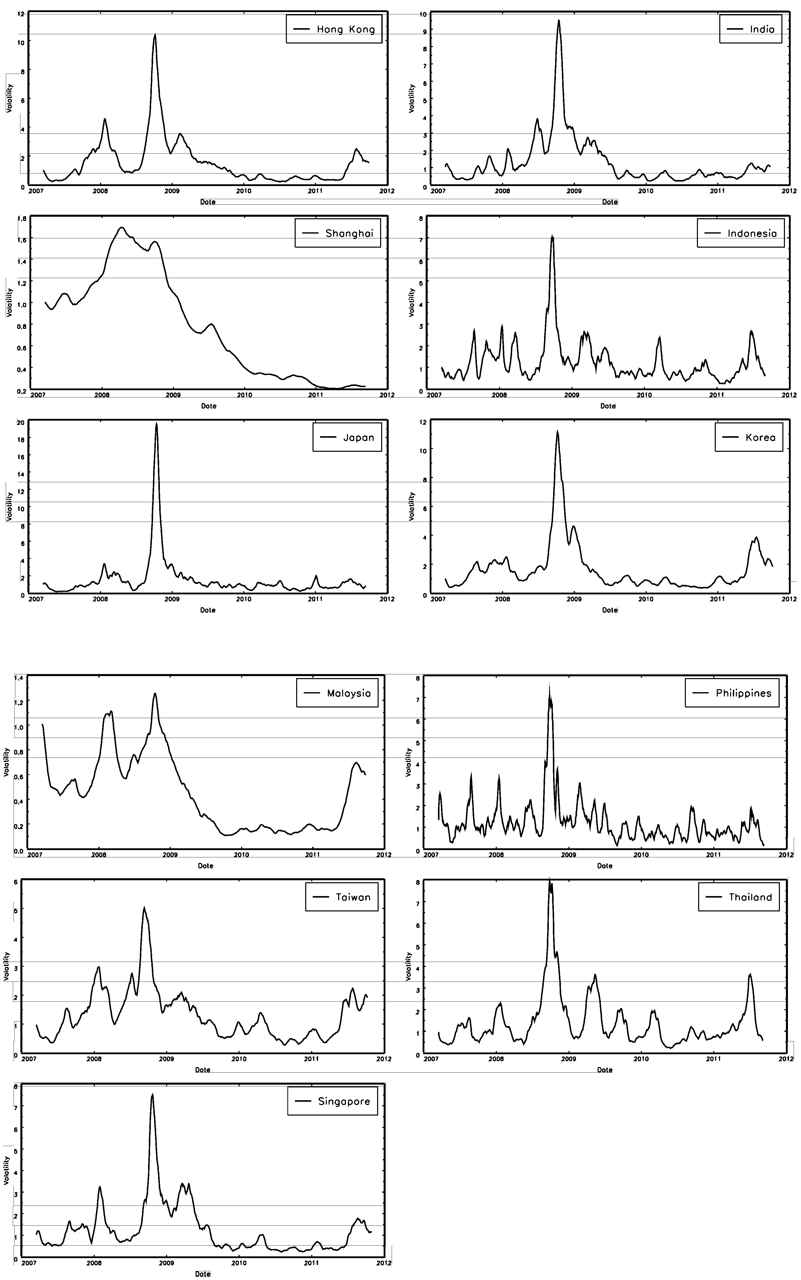
The rest of the paper is organized as follows. Section 2 details the framework and notation of the model. Section 3 proposes the formula of the test statistic for the linear state-space model. Section 4 reports the results of our Monte Carlo experiments for the empirical size and power of the test. In Section 5, the test is applied to the empirical analysis of the Asian stock market indexes. Section 6 briefly concludes this study. The derivation of the score functions and the conditional moments of state variables are given in Appendix.

2. Model

We here consider the following observation equations of the bivariate SV model:

$$\begin{array}{c}\hfill r_{1t}={\psi }_1\left(\frac{h_{1t}}{2}\right)e_{1t},r_{2t}={\psi }_2\left(\frac{h_{2t}}{2}\right)e_{2t}\end{array}$$

(1)

for series $k=1,2$ and time $t=1,\dots ,T$. Note that $r_{kt}$ is the observed variable, which typically denotes the demeaned rate of return on assets, $h_{kt}$ is demeaned part of log volatility, where $E\left(h_{kt}\right)=0$, $e_{kt}$ is an idiosyncratic noise with constant variance, standardized at 1, and $log{\psi }_k^2$ is the mean of log volatility, and hence ${\psi }_k$ is, roughly speaking, overall standard deviation of $r_{kt}$.

We linearize the observation equation to the linear state-space model (The log transformation breaks down when $r_{kt}=0$, since $log\left(0\right)=-\infty$. In practice, the use of $log(x+ϵ)-ϵ/(ϵ+x)$ has been suggested in place of $logx$ for small constant $ϵ>0$ to avoid this problem. This transformation is useful in that ϵ has no effect for large x. See Breidt and Carriquiry [10] for details.); taking log of squares of Equation (1), we have

$$\begin{array}{c}\hfill y_{1t}={\delta }_1+h_{1t}+{\xi }_{1t},y_{2t}={\delta }_2+h_{2t}+{\xi }_{2t}\end{array}$$

(2)

where $y_{kt}\equiv log{r}_{kt}^2,{\delta }_k\equiv log{\psi }_k^2+\mu ,{\xi }_{kt}\equiv log{e}_{kt}^2-\mu$, and $\mu \equiv E\left(log{e}_{kt}^2\right)$.

The main difference of our model from the original multivariate SV model is that Gaussianity of $({\xi }_1,{\xi }_2)$ is assumed in our model, namely

$$\begin{array}{c}\hfill \left[\begin{array}{c}{\xi }_{1t}\\ {\xi }_{2t}\end{array}\right]\sim \text{i.i.d.}N\left(\left[\begin{array}{c}0\\ 0\end{array}\right],\left[\begin{array}{cc}\eta & \eta \gamma \\ \eta \gamma & \eta \end{array}\right]\right)\end{array}$$

(3)

where γ is a correlation coefficient of $({\xi }_1,{\xi }_2)$, and hence the distribution of $e_{kt}$ is no longer Gaussian. We are not asserting that the log squared returns follow a Gaussian distribution in reality (As suggested by an anonymous reviewer, the distribution of $(e_{1t},e_{2t})$ under Gaussianity of $({\xi }_{1t},{\xi }_{2t})$ is, exactly speaking, inappropriate for market data. It can be easily shown that the marginal distribution of $e_{kt}$ is expressed as

$$f\left(e_{kt}\right)=\frac{1}{\sqrt{2\pi }\eta \left|e_{kt}\right|}exp\left[-\frac{{(log{e}_{kt}^2-\mu )}^2}{2\eta }\right],-\infty <e_{kt}<\infty$$

noting that $e_{kt}^2=exp(\mu +{\xi }_{kt})$ follows a log-normal distribution. It is easy to see that this distribution has zero density function at the origin.).

Under the assumption of Gaussianity of $(e_{1t},e_{2t})$, the model (1) would be a nonlinear non-Gaussian multivariate state space model; even conventional hypothesis testing for this model has been rarely calculated because of its heavy computational burden and complexity, and hence constructing a test for the number of factors, which is our aim, seems almost unfeasible under the original assumption.

It seems also algebraically unfeasible to derive a test statistics from Equation (2) if Gaussianity of $(e_{1t},e_{2t})$ is assumed. The properties of the linearized model under the Gaussianity assumption of ($e_{1t},e_{2t}$) was extensively studied by Harvey et al. [11] and they reported that their analytical expression is extremely complicated; for example, the joint covariance of $log{e}_{1t}^2$ and $log{e}_{2t}^2$ is expressed as an infinite series; the mean and variance of $log{e}_{kt}^2$ are expressed as $\mu =-1.27$ and $\eta ={\pi }^2/2\approx 4.93$, respectively.

On the other hand, the linearized model (2) is a linear state-space model under our assumption that the distribution of $({\xi }_{1t},{\xi }_{2t})$ is Gaussian and we can derive the score function and Fisher information, which are required to derive our test, though algebraically tedious, as shown in Appendix A.

The non-Gaussianity of $(e_{1t},e_{2t})$ in our model is a serious drawback if we use this model for asset pricing, where Gaussianity of return is an essential assumption. However, in the context of spillover or contagion in international finance, Gaussianity is not always an essential element. We believe that our assumption of Gaussian $({\xi }_{1t},{\xi }_{2t})$ is a cost to derive the test for a single volatility factor. The usefulness of our assumption can be tested by checking the usefulness of our test.

The observation equation density, namely the conditional density of $y_{1t}$ and $y_{2t}$ given $h_{1t}$ and $h_{2t}$, are expressed as

$$\begin{array}{cc}\hfill {\nu }_{1t}& \equiv f\left(y_{1t}\right|h_{1t})=\frac{1}{\sqrt{2\pi \eta }}exp\left[-\frac{{(y_{1t}-{\delta }_1-h_{1t})}^2}{2\eta }\right],\hfill \\ \hfill {\nu }_{2t}& \equiv f\left(y_{2t}\right|y_{1t},h_{1t},h_{2t})\hfill \\ & =\frac{1}{\sqrt{2\pi \eta (1-{\gamma }^2)}}exp\left(-\frac{{[(y_{2t}-{\delta }_2-h_{2t})-\gamma (y_{1t}-{\delta }_1-h_{1t})]}^2}{2\eta (1-{\gamma }^2)}\right).\hfill \end{array}$$

(4)

We here assume that the log volatilities follow the bivariate first-order autoregressive (AR) process:

$$\begin{array}{c}\hfill \begin{array}{cc}\hfill h_{1t}& ={\varphi }_1{h}_{1,t-1}+{\omega }_1^{1/2}{u}_{1,t-1},\left|{\varphi }_1\right|<1\hfill \\ \hfill h_{2t}& ={\varphi }_2{h}_{2,t-1}+\lambda {\omega }_1^{1/2}{u}_{1,t-1}+{\omega }_2^{1/2}{u}_{2,t-1},\left|{\varphi }_2\right|<1\hfill \end{array}\end{array}$$

(5)

where the idiosyncratic noise $u_t={(u_{1t},u_{2t})}^{\prime }$ follows Gaussian distribution, namely

$$\begin{array}{c}\hfill \left[\begin{array}{c}{u}_{1t}\\ u_{2t}\end{array}\right]\sim \text{i.i.d.}N\left(\left[\begin{array}{c}0\\ 0\end{array}\right],\left[\begin{array}{cc}1& 0\\ 0& 1\end{array}\right]\right).\end{array}$$

(6)

The transition Equation (5), or the conditional densities of $h_{1t}$ and $h_{2t}$ given their past values, are expressed as

$$\begin{array}{cc}\hfill {\tau }_{1t}& \equiv f\left(h_{1t}\right|h_{1,t-1})=\frac{1}{\sqrt{2\pi {\omega }_1}}exp\left[-\frac{{(h_{1t}-{\varphi }_1{h}_{1,t-1})}^2}{2{\omega }_1}\right],\hfill \\ \hfill {\tau }_{2t}& \equiv f\left(h_{2t}\right|h_{1t},h_{1,t-1},h_{2,t-1})\hfill \\ & =\frac{1}{\sqrt{2\pi {\omega }_2}}exp\left(-\frac{{[(h_{2t}-{\varphi }_2{h}_{2,t-1})-\lambda (h_{1t}-{\varphi }_1{h}_{1,t-1})]}^2}{2{\omega }_2}\right).\hfill \end{array}$$

(7)

This formulation is not a general bivariate autoregressive process in that they are two univariate first-order AR processes with correlated innovations (Harvey et al. [11] set ${\varphi }_1,{\varphi }_2$ to unity.). The general condition for the identity $h_{1t}=h_{2t}$ is that the coefficient matrix of the multivariate first-order AR model has eigenvector ${(1,1)}^{\prime }$, in addition to the degeneracy of disturbances. However, we believe that our assumption is sufficient for practical use.

Then, the density function of ${\tilde{y}}_T\equiv {(y_{11},y_{21},\dots ,y_{1T},y_{2T})}^{\prime }$, or the likelihood function, from which our LM test statistic is derived, is expressed as follows:

$$\begin{array}{c}\hfill f\left({\tilde{y}}_T\right)={\int }_{-\infty }^{\infty }\cdots {\int }_{-\infty }^{\infty }f({\tilde{y}}_T,{\tilde{h}}_T)d{h}_{11}d{h}_{21}\cdots d{h}_{1T}d{h}_{2T}\end{array}$$

(8)

by integrating out the state variables ${\tilde{h}}_T\equiv {(h_{11},h_{21},\dots ,h_{1T},h_{2T})}^{\prime }$, where

$$f({\tilde{y}}_T,{\tilde{h}}_T)=\prod _{t=1}^T\prod _{k=1}^2{\nu }_{kt}{\tau }_{kt}.$$

We have two notes for the integration in Equation (8). First, our model defined by Equations (2), (3), (5), and (6) is linear and Gaussian, and hence the likelihood function can be evaluated and maximized, without numerical integration, whether by means of quadrature or Monte Carlo methods. Hence, we evaluate the likelihood by means of the Kalman filter method, which was suggested by Nelson [12] and Harvey et al. [11]. Second, the transition density is degenerate under the null hypothesis and the integration can be performed by integration by parts, as shown in Appendix A.

In the conventional multivariate SV model, which is different from ours, the observation equation disturbance term $e_t={(e_{1t},e_{2t})}^{\prime }$ follows Gaussian distribution:

$$\begin{array}{c}\hfill \left[\begin{array}{c}{e}_{1t}\\ e_{2t}\end{array}\right]\sim \text{i.i.d.}N\left(\left[\begin{array}{c}0\\ 0\end{array}\right],\left[\begin{array}{cc}1& \rho \\ \rho & 1\end{array}\right]\right).\end{array}$$

(9)

Harvey et al. [11] showed that the maximum likelihood (ML) estimator of this transformed model, which is called the quasi-maximum likelihood estimator (QMLE), is consistent under the original assumption of the Gaussianity of $e_t$. The estimation of SV model in the original form (9) can be carried out by various methods, for example, the generalized method of moments (GMM) used by Melino and Turnbull [13], the efficient method of moments (EMM) applied by Gallant et al. [14], and Markov Chain Monte Carlo (MCMC) procedures used by Jacquier et al. [6] and Kim et al. [7]. The construction of tests for the original model (9) based upon these methods is left for further research. However, little attention has been paid to hypothesis testing of this model.

3. Test Statistic

We propose the LM test for the hypothesis that the observation series $y_{1t}$ and $y_{2t}$ have the only stochastic volatility factor in common, and other idiosyncratic volatility factors are negligible, namely $h_{1t}=h_{2t}$ for any t in Equation (5), against the alternative hypothesis that each series has different, possibly correlated, log volatility series $h_{1t}$ and $h_{2t}$.

The null hypothesis that $h_{1t}=h_{2t}$ is a first order approximation to the international synchronization of asset price fluctuation, found, or believed to be found, in the period that includes financial crises. In normal periods actual volatilities of markets are expressed as mixtures of many factors. In the period that includes financial crises, however, only a single intermarket volatility factor may override other minor volatility factors in markets. In such an extreme situation, other minor domestic volatility factors are negligible in size and some markets look as if they have a single common volatility factor. The aim of our test is not to assert there exists only a single volatility factor among markets, but is to check whether minor volatility factors are negligible in comparison with a big intermarket volatility factor.

In our Equation (7), the innovations are perfectly correlated if ${\omega }_2=0$, and mutually independent if ${\omega }_2=\infty$. Our test checks that the two series have the same autoregressive coefficient and innovation variance, namely ${\varphi }_1={\varphi }_2,\lambda =1$, as well as the degeneracy of the innovation, namely ${\omega }_2=0$. Therefore, in Equation (5), the null hypothesis is formalized as

$$\begin{array}{c}\hfill H_0:{\varphi }_1={\varphi }_2,\lambda =1,{\omega }_2=0.\end{array}$$

(10)

In our framework, in order to define the existence of a single overriding volatility factor in two markets, the volatility series of two markets should be exactly the same, which means ${\varphi }_1={\varphi }_2$, $\lambda =1$, ${\omega }_2=0$, and hence $h_{1t}=h_{2t}$, when the volatility series is stationary; the logic is as follows: If the volatility processes of two market are not identical but correlated by assuming ${\omega }_2\ne 0$, they have different volatility shocks and hence volatility series have different patterns especially when the absolute value of ${\omega }_2$ is large, then we have no choice than to define the number of volatility factors in the market is two when ${\omega }_2\ne 0$. Then the condition ${\omega }_2=0$, or very small absolute value of ${\omega }_2$, is a essential element in defining the single overriding volatility series. When ${\omega }_2=0$, we need the condition ${\varphi }_1={\varphi }_2$, to define the single overriding volatility series, since ${\varphi }_1\ne {\varphi }_2$ implies different cyclicality or periodicity of volatility process.

It is arguable whether the condition $\lambda =1$ is necessary. Under the assumption of ${\omega }_2=0$, the condition $0<\lambda <1$ expresses smaller variance of $h_{2t}$ than that of $h_{1t}$ around 0 and hence, intuitively, smaller variance of $exp\left(h_{2t}\right)$ than that of $exp\left(h_{1t}\right)$ around 1, namely variance of volatility of $r_{1t}$, disregarding proportionality constant $exp\left({\delta }_1\right)$. Then λ can be regarded as “volatility of volatility” parameter and hence should be 1 if two markets follow the same volatility factor. If the same volatility process implies identical volatility of volatility, we need the condition $\lambda =1$.

We need the initial value condition $h_{10}=h_{20}$ additionally for the log volatilities to be exactly identical stochastic processes under the conditions of (10). However, the log volatilities converge to zero quickly as long as they are stationary, even if their initial values are different, and the effect of $(h_{10},h_{20})$ disappears in the vector moving average expression of $h_{kt}$, as t increases. Then, we only consider the conditions (10) hereafter.

The Wald and Likelihood ratio principles are irrelevant to test for Equation (10), because the maximum likelihood estimator of ${\omega }_2$ can have a singular distribution under the null hypothesis; the parameter value ${\omega }_2=0$ under the null is on the boundary of the parameter space ${\omega }_2\ge 0$, so that their estimators cannot have an asymptotically normal distribution. The LM test is free from the boundary value problem, since it forgoes estimation of the constrained parameter ${\omega }_2$;

We now restate the null hypothesis (10), by the parameter transformation ${\rho }_1={\varphi }_1,{\rho }_2={\varphi }_2-{\varphi }_1,$ to

$$\begin{array}{c}\hfill H_0:{\rho }_2=0,\lambda =1,{\omega }_2=0;\end{array}$$

(11)

the original parameter vector $\vartheta ={({\delta }_1,{\delta }_2,\eta ,\gamma ,{\varphi }_1,{\varphi }_2,{\omega }_1,{\omega }_2,\lambda )}^{\prime }$ is transformed into the new parameter vector $\theta ={({\delta }_1,{\delta }_2,\eta ,\gamma ,{\rho }_1,{\rho }_2,{\omega }_1,{\omega }_2,\lambda )}^{\prime }$. The vectors of the restricted and unrestricted parameters are denoted by ${\theta }_1={({\rho }_2,{\omega }_2,\lambda )}^{\prime }$, ${\theta }_2=({\delta }_1,{\delta }_2,\eta ,\gamma ,{\rho }_1,{\omega }_1{)}^{\prime }$ respectively, and the log likelihood function for θ is denoted by $\mathcal{L}\left(\theta \right)\equiv logf\left({\tilde{y}}_T\right),$ using the likelihood function defined in Equation (8). Then, the LM test statistic for Equation (11) is defined as

$$\begin{array}{c}\hfill LM=s_1^{\prime }\left(\widehat{\theta }\right)I_{OP}^{11}\left(\widehat{\theta }\right)s_1\left(\widehat{\theta }\right)\end{array}$$

(12)

where the derivative of $\mathcal{L}\left(\theta \right)$ with respect to ${\theta }_1$ is denoted by

$$\begin{array}{c}\hfill s_1\left(\widehat{\theta }\right)=\frac{\partial \mathcal{L}\left(\widehat{\theta }\right)}{\partial {\theta }_1}\end{array}$$

(13)

evaluated at $\widehat{\theta }$, namely the maximum likelihood estimator of θ under the null hypothesis, and $I_{OP}^{11}\left(\widehat{\theta }\right)$ is the upper-left three-by-three submatrix of the inverse of the Fisher information matrix evaluated at $\widehat{\theta }$. Then, the LM test statistic follows asymptotically ${\chi }^2$ distribution with three degrees of freedom, which is the number of constraints.

The Fisher information can be calculated by

$$I_{OP}\left(\theta \right)={\mathrm{E}}_0\left(\sum _{t=1}^T{\ell }_t{\ell }_t^{\prime }\right)$$

(14)

where

$${\ell }_t=\frac{\partial logf\left({\tilde{y}}_t\right)}{\partial \theta }-\frac{\partial logf\left({\tilde{y}}_{t-1}\right)}{\partial \theta }$$

as shown by Hamilton [15] from the identity

$${\ell }_t=\frac{\partial logf\left({\tilde{y}}_t\right|{\tilde{y}}_{t-1})}{\partial \theta }.$$

In practice, $I_{OP}^{11}\left(\theta \right)$ is estimated by ${\sum }_{t=1}^T{\ell }_t{\ell }_t^{\prime }$ where the unknown parameters θ are estimated by the maximum likelihood method under the null hypothesis.

Hence, we have only to derive the score functions, or the derivatives of log of $f\left({\tilde{y}}_T\right)$ in Equation (8) with respect to θ, to calculate the LM test statistics using Equations (13) and (14). Their derivation is straightforward, by means of integration by parts, but very lengthy so that we provide the detailed derivation in Appendix A.

Denoting ${\mathrm{E}}_0$ as the expectation under the null hypothesis, their score functions evaluated under the null hypothesis are as follows:

$$\begin{array}{cc}\hfill \frac{\partial \mathcal{L}\left(\widehat{\theta }\right)}{\partial {\rho }_1}& =\sum _{t=2}^T\frac{{\mathrm{E}}_0\left(h_{t-1}{u}_{1,t-1}\right|{\tilde{y}}_T)}{{\widehat{\omega }}_1},\frac{\partial \mathcal{L}\left(\widehat{\theta }\right)}{\partial {\rho }_2}=\sum _{t=2}^T\sum _{j=t}^T{\widehat{\varphi }}_2^{j-t}\left[\frac{{\mathrm{E}}_0\left(h_{t-1}{\xi }_{2j}\right|{\tilde{y}}_T)-\widehat{\gamma }{\mathrm{E}}_0\left(h_{t-1}{\xi }_{1j}\right|{\tilde{y}}_T)}{\widehat{\eta }(1-{\widehat{\gamma }}^2)}\right],\hfill \\ \hfill \frac{\partial \mathcal{L}\left(\widehat{\theta }\right)}{\partial \lambda }& =\sum _{t=2}^T\sum _{j=t}^T{\widehat{\varphi }}_2^{j-t}\left[\frac{{\mathrm{E}}_0\left(u_{1,t-1}{\xi }_{2j}\right|{\tilde{y}}_T)-\widehat{\gamma }{\mathrm{E}}_0\left(u_{1,t-1}{\xi }_{1j}\right|{\tilde{y}}_T)}{\widehat{\eta }(1-{\widehat{\gamma }}^2)}\right],\hfill \\ \hfill \frac{\partial \mathcal{L}\left(\widehat{\theta }\right)}{\partial {\widehat{\omega }}_2}& =\sum _{t=1}^T\sum _{k=1}^t{\widehat{\varphi }}_2^{2(k-1)}\left[\frac{{\mathrm{E}}_0\left({\xi }_{2t}^2\right|{\tilde{y}}_T)-2\widehat{\gamma }{\mathrm{E}}_0\left({\xi }_{2t}{\xi }_{1t}\right|{\tilde{y}}_T)+{\widehat{\gamma }}^2{\mathrm{E}}_0\left({\xi }_{1t}^2\right|{\tilde{y}}_T)}{{\widehat{\eta }}^2{(1-{\widehat{\gamma }}^2)}^2}-\frac{1}{\widehat{\eta }(1-{\widehat{\gamma }}^2)}\right]\hfill \\ & +\sum _{t=1}^{T-1}\sum _{k=t}^{T-1}{\widehat{\varphi }}_2^{2(k-t)}\sum _{l=k+1}^T{\widehat{\varphi }}_2^{l-k}\left[\frac{{\mathrm{E}}_0\left({\xi }_{2k}{\xi }_{2l}\right|{\tilde{y}}_T)-\widehat{\gamma }{\mathrm{E}}_0\left({\xi }_{2k}{\xi }_{1l}\right|{\tilde{y}}_T)-\widehat{\gamma }{\mathrm{E}}_0\left({\xi }_{2l}{\xi }_{1k}\right|{\tilde{y}}_T)+{\widehat{\gamma }}^2{\mathrm{E}}_0\left({\xi }_{1k}{\xi }_{1l}\right|{\tilde{y}}_T)}{{\widehat{\eta }}^2{(1-{\widehat{\gamma }}^2)}^2}\right],\hfill \end{array}$$

$$\begin{array}{cc}\hfill \frac{\partial \mathcal{L}\left(\widehat{\theta }\right)}{\partial {\delta }_1}& =\sum _{t=1}^T\frac{{\mathrm{E}}_0\left({\xi }_{1t}\right|{\tilde{y}}_T)-\widehat{\gamma }{\mathrm{E}}_0\left({\xi }_{2t}\right|{\tilde{y}}_T)}{\widehat{\eta }(1-{\widehat{\gamma }}^2)},\frac{\partial \mathcal{L}\left(\widehat{\theta }\right)}{\partial {\delta }_2}=\sum _{t=1}^T\frac{{\mathrm{E}}_0\left({\xi }_{2t}\right|{\tilde{y}}_T)-\widehat{\gamma }{\mathrm{E}}_0\left({\xi }_{1t}\right|{\tilde{y}}_T)}{\widehat{\eta }(1-{\widehat{\gamma }}^2)},\hfill \\ \hfill \frac{\partial \mathcal{L}\left(\widehat{\theta }\right)}{\partial \eta }& =\sum _{t=1}^T\left\{\left(\frac{1}{2}\right)\left[\frac{E_0\left({\xi }_{2t}^2\right|\tilde{y})-2\widehat{\gamma }{E}_0\left({\xi }_{1t}{\xi }_{2t}\right|\tilde{y})+E_0\left({\xi }_{1t}^2\right)}{{\widehat{\eta }}^2(1-{\widehat{\gamma }}^2)}\right]-\left(\frac{1}{\widehat{\eta }}\right)\right\},\hfill \\ \hfill \frac{\partial \mathcal{L}\left(\widehat{\theta }\right)}{\partial \gamma }& =\sum _{t=1}^T\left[\left(\frac{\widehat{\gamma }}{1-{\widehat{\gamma }}^2}\right)-\frac{\widehat{\gamma }{\mathrm{E}}_0\left({\xi }_{1t}^2\right|{\tilde{y}}_T)+\widehat{\gamma }{\mathrm{E}}_0\left({\xi }_{2t}^2\right|{\tilde{y}}_T)-(1+{\widehat{\gamma }}^2){\mathrm{E}}_0\left({\xi }_{1t}{\xi }_{2t}\right|{\tilde{y}}_T)}{\widehat{\eta }{(1-{\widehat{\gamma }}^2)}^2}\right],\hfill \\ \hfill \frac{\partial \mathcal{L}\left(\widehat{\theta }\right)}{\partial {\widehat{\omega }}_1}& =\left(\frac{1}{2}\right)\sum _{t=2}^T\left[\frac{{\mathrm{E}}_0\left(u_{1,t-1}^2\right|{\tilde{y}}_T)}{{\widehat{\omega }}_1^2}-\left(\frac{1}{{\widehat{\omega }}_1}\right)\right].\hfill \end{array}$$

Denoting $m_t={\mathrm{E}}_0\left(h_t\right|{\tilde{y}}_T),c_{ts}={\mathrm{E}}_0\left(h_t{h}_s\right|{\tilde{y}}_T)$, the conditional moments of ${\xi }_{1t},{\xi }_{2t},u_{1t},h_t$ given ${\tilde{y}}_T$ under the null hypothesis can be expressed as

$${\mathrm{E}}_0\left(\left.h_{t-1}{u}_{1,t-1}\right|{\tilde{y}}_T\right)=c_{t-1,t}-{\widehat{\varphi }}_1{c}_{t-1,t-1},{\mathrm{E}}_0\left(\left.u_{1,t-1}^2\right|{\tilde{y}}_T\right)=c_{tt}-2{\widehat{\varphi }}_1{c}_{t-1,t}+{\widehat{\varphi }}_1^2{c}_{t-1,t-1},$$

$${\mathrm{E}}_0\left(\left.h_{t-1}{\xi }_{1j}\right|{\tilde{y}}_T\right)=m_{t-1}(y_{1j}-{\widehat{\delta }}_1)-c_{t-1,j},{\mathrm{E}}_0\left(\left.h_{t-1}{\xi }_{2j}\right|{\tilde{y}}_T\right)=m_{t-1}(y_{2j}-{\widehat{\delta }}_2)-c_{t-1,j},$$

$${\mathrm{E}}_0\left(\left.{\xi }_{1t}\right|{\tilde{y}}_T\right)=y_{1j}-{\widehat{\delta }}_1-m_t,{\mathrm{E}}_0\left(\left.{\xi }_{2t}\right|{\tilde{y}}_T\right)=y_{2j}-{\widehat{\delta }}_2-m_t,$$

$${\mathrm{E}}_0\left(\left.{\xi }_{1k}{\xi }_{2l}\right|{\tilde{y}}_T\right)=(y_{1k}-{\widehat{\delta }}_1)(y_{2l}-{\widehat{\delta }}_2)-m_k(y_{2l}-{\widehat{\delta }}_2)-(y_{1k}-{\widehat{\delta }}_1)m_l+c_{kl}$$

from Equations (2) and (5). See Appendix B for their derivation.

4. Monte Carlo Experiments

To examine the performance of our proposed test, we conduct Monte Carlo experiments using the GAUSS programming language. We use the following data generating process:

• Generate $\left\{e_{kt}^2\right\}$ from multivariate log-normal random number generator from GAUSS library (The joint probability density function of $e_{1t}^2$ and $e_{2t}^2$ is expressed as

  $$\begin{array}{cc}\hfill f(e_{1t}^2,e_{2t}^2)& =\frac{1}{\left(2\pi \right)\sqrt{{\eta }^2({\gamma }^2-1)}{e}_{1t}^2{e}_{2t}^2}\hfill \\ & \times exp\left[\frac{\eta \gamma {(log{e}_{1t}^2-\mu )}^2-2\eta (log{e}_{1t}^2-\mu )(log{e}_{2t}^2-\mu )+\eta \gamma {(log{e}_{2t}^2-\mu )}^2}{{\eta }^2({\gamma }^2-1)}\right]\hfill \end{array}$$

  for $0<e_{1t}^2,e_{2t}^2<\infty$. Note that the library name of multivariate log-normal random number generator in GAUSS is $rndLogNorm(·,·,·,·)$.). In addition, generate $\left\{u_{kt}\right\}$ from Gaussian random number generator.
• Generate $\left\{r_{kt}^2\right\},\left\{h_{kt}\right\}$ from $\left\{e_{kt}^2\right\},\left\{u_{kt}\right\}$. The processes of $\left\{r_{kt}^2\right\}$ and $\left\{h_{kt}\right\}$ are obtained from the following model;

  $$\begin{array}{cc}\hfill \left[\begin{array}{c}{r}_{1t}^2\\ r_{2t}^2\end{array}\right]& =\left[\begin{array}{cc}{\psi }_1^{2}exp\left(h_{1t}\right)& 0\\ 0& {\psi }_2^{2}exp\left(h_{2t}\right)\end{array}\right]\left[\begin{array}{c}{e}_{1t}^2\\ e_{2t}^2\end{array}\right],\hfill \end{array}$$

  $$\begin{array}{cc}\hfill \left[\begin{array}{c}{h}_{1t}\\ h_{2t}\end{array}\right]& =\left[\begin{array}{cc}{\varphi }_1& 0\\ 0& {\varphi }_2\end{array}\right]\left[\begin{array}{c}{h}_{1,t-1}\\ h_{2,t-1}\end{array}\right]+\left[\begin{array}{cc}{\omega }_1^{1/2}& 0\\ \lambda {\omega }_1^{1/2}& {\omega }_2^{1/2}\end{array}\right]\left[\begin{array}{c}{u}_{1,t-1}\\ u_{2,t-1}\end{array}\right]\hfill \end{array}$$

  for $t=1,\dots ,T$.
• Calculate ${\delta }_k$ from ${\delta }_k=\mu +log{\psi }_k^2$ and generate $\left\{y_{kt}\right\},\left\{{\xi }_{kt}\right\}$ from $y_{kt}=log{r}_{kt}^2,{\xi }_{kt}=log{e}_{kt}^2-\mu$, respectively.

From the above data generating process, we can define the following linear Gaussian state-space model:

• Observation equation

  $$\left[\begin{array}{c}{y}_{1t}\\ y_{2t}\end{array}\right]=\left[\begin{array}{c}{\delta }_1\\ {\delta }_2\end{array}\right]+\left[\begin{array}{c}{h}_{1t}\\ h_{2t}\end{array}\right]+\left[\begin{array}{c}{\xi }_{1t}\\ {\xi }_{2t}\end{array}\right],$$
• Transition equation

  $$\left[\begin{array}{c}{h}_{1t}\\ h_{2t}\end{array}\right]=\left[\begin{array}{cc}{\varphi }_1& 0\\ 0& {\varphi }_2\end{array}\right]\left[\begin{array}{c}{h}_{1,t-1}\\ h_{2,t-1}\end{array}\right]+\left[\begin{array}{cc}{\omega }_1^{1/2}& 0\\ \lambda {\omega }_1^{1/2}& {\omega }_2^{1/2}\end{array}\right]\left[\begin{array}{c}{u}_{1,t-1}\\ u_{2,t-1}\end{array}\right],$$
• Structure of innovation distribution

  $$\left[\begin{array}{c}{\xi }_{1t}\\ {\xi }_{2t}\\ u_{1t}\\ u_{2t}\end{array}\right]\sim \text{i.i.d.}N\left(\left[\begin{array}{c}0\\ 0\\ 0\\ 0\end{array}\right],\left[\begin{array}{cccc}\eta & \eta \gamma & 0& 0\\ \eta \gamma & \eta & 0& 0\\ 0& 0& 1& 0\\ 0& 0& 0& 1\end{array}\right]\right),\text{for}t=1,\dots ,T.$$

We here report the simulation at $\mu =-1.27,\eta ={\pi }^2/2,\gamma =0.1,{\psi }_1=1,{\psi }_2=1,{\varphi }_1=0.7,{\varphi }_2=0.7,{\omega }_1=0.1,{\omega }_2=0,\lambda =1$ and its neighborhood (Note that the parameters $(\mu ,\eta ,{\psi }_1,{\psi }_2)$ are fixed at $(-1.27,{\pi }^2/2,1,1)$ throughout this experiment. Then, ${\delta }_k$ is expressed simply as ${\delta }_k=\mu +log{1}^2=-1.27$.). In this experiments, the number of replications is 1000, the sample sizes are $T=500,750$, and the initial value of $(h_{1t},h_{2t},u_{1t},u_{2t})$ are fixed at $(1,1,0,0)$ respectively. The initial value of parameters for ML estimation are ${\delta }_1^{\left(0\right)}=0,{\delta }_2^{\left(0\right)}=0,{\eta }^{\left(0\right)}={\pi }^2/2,{\gamma }^{\left(0\right)}=0,{\varphi }_1^{\left(0\right)}=0.9,{\varphi }_2^{\left(0\right)}=0.9,{\omega }_1^{\left(0\right)}=0.1,{\omega }_2^{\left(0\right)}=0,{\lambda }^{\left(0\right)}=1$. Finally, we generate $T+100$ periods of data and use the last T periods by discarding the first 100 periods to reduce the effect of initial values. The procedure (See Durbin and Koopman [16] for a detailed discussion and review of the algorithm of the Kalman filter and smoother.) works as follows.

• Apply the Kalman filtering to $\left\{y_t\right\}$ under the null hypothesis (10) and estimate the parameters by the maximum likelihood (ML) method.
• Apply the smoothing algorithm to $\left\{y_t\right\}$ and obtain the conditional moments of $\left\{h_t\right\}$.
• Calculate the LM test statistic (12).

Table 1 gives the empirical size of the test, namely the rejection rate of the null hypothesis, under the null for some values of the correlation coefficient γ in Equation (4), the autocorrelation coefficient and variance of the transition equation, namely ${\varphi }_1$ and ${\omega }_1$ in Equation (7). Table 2 reports the empirical power of the test, when the two series have different log volatility series, with different autocorrelation coefficients ${\varphi }_1$ and ${\varphi }_2$, or nondegenerate innovations with nonzero value of ${\omega }_2$ in Equation (7). Each table reports the percentage rate of rejection of the relevant null hypothesis at the asymptotic 5% and 1% significance level. Note that the rejection region of the tests are in the upper tail areas. Our main findings are summarized as follows.

• Size of the test: For $T=500$, the actual size of the test deviates from the nominal sizes of 5 and 1 percent at most by 3.1 and 1.9 percent, respectively. In particular, when the estimated volatility series are strongly correlated and can be characterized as near unit root processes, the size distortion are increasing. As the sample size increases, namely when $T=750$, the actual rejection rate is closer to the nominal level, as is expected.
• Power under the alternative: For $T=500$, the rejects rate of the null ranges from 12.9 percent to 58.9 percent for the nominal 5 percent significance level. As the sample size increases, the actual rejection rate is increasing. This results indicate that the absolute value of the difference between the null and the alternative is 0.2 or more, the test statistics can discriminate the hypothesis.

Table 1. Empirical size of the LM test by Monte Carlo experiments.

γ	${\varphi }_1$	${\omega }_1$	$T=500$		$T=750$
			5%	1%	5%	1%
0.1	0.7	0.1	6.1	1.2	5.5	0.9
0	0.7	0.1	5.8	1.9	5.3	1.2
−0.1	0.7	0.1	4.6	0.8	5.1	1.1
0.1	0.9	0.1	7.2	1.8	5.7	1.4
0.1	0.95	0.1	8.1	2.9	6.5	1.8
0.1	0.7	0.2	7.1	1.6	5.4	1.1
0.1	0.7	0.3	5.1	0.7	4.9	1.2

Note: The number of replications is 1000. We set ${\varphi }_1={\varphi }_2,\lambda =1,{\omega }_2=0$ throughout this experiment.

Table 1. Empirical size of the LM test by Monte Carlo experiments.

γ	${\varphi }_1$	${\omega }_1$	$T=500$		$T=750$
			5%	1%	5%	1%
0.1	0.7	0.1	6.1	1.2	5.5	0.9
0	0.7	0.1	5.8	1.9	5.3	1.2
−0.1	0.7	0.1	4.6	0.8	5.1	1.1
0.1	0.9	0.1	7.2	1.8	5.7	1.4
0.1	0.95	0.1	8.1	2.9	6.5	1.8
0.1	0.7	0.2	7.1	1.6	5.4	1.1
0.1	0.7	0.3	5.1	0.7	4.9	1.2

Note: The number of replications is 1000. We set ${\varphi }_1={\varphi }_2,\lambda =1,{\omega }_2=0$ throughout this experiment.

Table 2. Empirical power of the LM test by Monte Carlo experiments.

${\varphi }_2$	λ	${\omega }_2$	$T=500$		$T=750$
			5%	1%	5%	1%
0.5	1	0	25.5	10.7	36.9	17.7
0.9	1	0	39.0	18.4	52.3	24.6
0.7	0.8	0	12.9	1.3	15.1	5.1
0.7	0.6	0	31.5	14.1	44.4	20.9
0.7	1	0.2	17.9	5.5	24.9	9.0
0.7	1	0.4	58.9	32.3	79.1	52.3

The number of replications is 1000. We set $\gamma =0.1,{\varphi }_1=0.7,{\omega }_1=0.1$ throughout this experiment.

Table 2. Empirical power of the LM test by Monte Carlo experiments.

${\varphi }_2$	λ	${\omega }_2$	$T=500$		$T=750$
			5%	1%	5%	1%
0.5	1	0	25.5	10.7	36.9	17.7
0.9	1	0	39.0	18.4	52.3	24.6
0.7	0.8	0	12.9	1.3	15.1	5.1
0.7	0.6	0	31.5	14.1	44.4	20.9
0.7	1	0.2	17.9	5.5	24.9	9.0
0.7	1	0.4	58.9	32.3	79.1	52.3

The number of replications is 1000. We set $\gamma =0.1,{\varphi }_1=0.7,{\omega }_1=0.1$ throughout this experiment.

An important practical conclusion of our simulation is that a rather large sample size, such as more than $T=500$, is necessary to distinguish the null and the alternative. However, datasets with a sample size of 500 or more are easily available in financial analyses.

Summarizing, Monte Carlo results showed that the tests are reliable in terms of both size and power performance.

5. Empirical Analysis

5.1. Univariate Analysis

5.1.1. Data and Descriptive Statistics

We apply the proposed test to the Asian stock market indexes to study volatility spillover in this area. We use daily data (The data will be available from the first author upon request.) of the eleven stock indexes for an about 5-year period from February 23, 2007 to December 8, 2011, excluding the periods when the markets are closed, downloaded from Datastream. For each index, we have a series consisting of 1,250 days. Table 3 gives a complete list of their ticker symbols, index names, and the corresponding markets. These stock market indexes are transformed into daily rates of return. The daily return of index i at time t is calculated as

$$r_{it}=log{p}_{it}-log{p}_{i,t-1}$$

where $p_{it}$ denotes the price of index i at time t. In Table 4, the univariate statistics for the returns in percentage terms are presented. The mean for each return is on average around 0.006 percent, while the standard deviation is around 1.704 percent. Mean return of Indonesia is higher than that of the other ten indexes. The return of Hong Kong has the highest volatility among the eleven, whereas the return of Malaysia has the lowest.

Table 3. Ticker symbols, Index names, and the corresponding markets.

Index Number	Ticker	Index name	Market
1	HKSPLCI	S&P/HKEx Large Cap Index	Hong Kong (HKG)
2	IBOMBSE	BSE 100 Index	India (IND)
3	CHSASHR	Shanghai Stock Exchange A Share Index	Shanghai (SHA)
4	JAKCOMP	Jakarta Stock Exchange Composite Index	Indonesia (IDN)
5	JAPDOWA	Nikkei 225 Stock Average Index	Japan (JPN)
6	KOR200I	Korea Stock Exchange KOSPI 200 Index	Korea (KOR)
7	FBMKLCI	FTSE Bursa Malaysia KLCI Index	Malaysia (MYS)
8	PSECOMP	Philippines Stock Exchange PSEi Index	Philippines (PHL)
9	TAIWGHT	FTSE TWSE Taiwan 50 Index	Taiwan (TWN)
10	BNGKS50	Stock Exchange of Thailand SET 50 Index	Thailand (THA)
11	SNGPORI	FTSE Straits Times Index	Singapore (SGP)

Table 3. Ticker symbols, Index names, and the corresponding markets.

Index Number	Ticker	Index name	Market
1	HKSPLCI	S&P/HKEx Large Cap Index	Hong Kong (HKG)
2	IBOMBSE	BSE 100 Index	India (IND)
3	CHSASHR	Shanghai Stock Exchange A Share Index	Shanghai (SHA)
4	JAKCOMP	Jakarta Stock Exchange Composite Index	Indonesia (IDN)
5	JAPDOWA	Nikkei 225 Stock Average Index	Japan (JPN)
6	KOR200I	Korea Stock Exchange KOSPI 200 Index	Korea (KOR)
7	FBMKLCI	FTSE Bursa Malaysia KLCI Index	Malaysia (MYS)
8	PSECOMP	Philippines Stock Exchange PSEi Index	Philippines (PHL)
9	TAIWGHT	FTSE TWSE Taiwan 50 Index	Taiwan (TWN)
10	BNGKS50	Stock Exchange of Thailand SET 50 Index	Thailand (THA)
11	SNGPORI	FTSE Straits Times Index	Singapore (SGP)

Table 5 also shows the Ljung-Box statistics to test the null of hypothesis absence of serial correlation in both the levels ($LB$) and in the squares ($L{B}^2$) until the 15 lag. Note that the squared returns are used as an approximation to each index’s volatility. The returns in levels show a certain degree of serial correlation, since for eight out of eleven cases, we reject the null hypothesis. Furthermore, all the $L{B}^2$ test on the squared returns indicate the precense of serial correlation at any significance level and, therefore the existence of volatility clustering. In this case, the theoretical distribution of the Ljung-Box test is not correct and there is a tendency to over-reject the null.

Table 4. Univariate statistics for the daily index returns.

Market	Max	Min	Mean	Median	Standard Deviation	Skewness	Kurtosis
Hong Kong	13.353	−13.459	−0.004	0.057	2.070	0.088	8.696
India	15.490	−11.689	0.019	0.096	1.912	0.022	9.343
Shanghai	9.033	−9.261	−0.022	0.109	2.020	−0.366	5.448
Indonesia	7.623	−10.954	0.064	0.181	1.740	−0.635	8.652
Japan	13.235	−12.111	−0.063	0.015	1.876	−0.495	10.559
Korea	11.540	−10.903	0.023	0.121	1.753	−0.422	8.303
Malaysia	4.259	−9.979	0.012	0.054	0.958	−1.223	14.945
Philippines	9.365	−13.089	0.021	0.056	1.550	−0.773	10.882
Taiwan	6.525	−6.735	−0.009	0.110	1.549	−0.342	5.054
Thailand	8.916	−12.563	0.036	0.053	1.782	−0.477	8.384
Singapore	7.531	−8.696	−0.014	0.012	1.533	−0.118	6.576

Table 4. Univariate statistics for the daily index returns.

Market	Max	Min	Mean	Median	Standard Deviation	Skewness	Kurtosis
Hong Kong	13.353	−13.459	−0.004	0.057	2.070	0.088	8.696
India	15.490	−11.689	0.019	0.096	1.912	0.022	9.343
Shanghai	9.033	−9.261	−0.022	0.109	2.020	−0.366	5.448
Indonesia	7.623	−10.954	0.064	0.181	1.740	−0.635	8.652
Japan	13.235	−12.111	−0.063	0.015	1.876	−0.495	10.559
Korea	11.540	−10.903	0.023	0.121	1.753	−0.422	8.303
Malaysia	4.259	−9.979	0.012	0.054	0.958	−1.223	14.945
Philippines	9.365	−13.089	0.021	0.056	1.550	−0.773	10.882
Taiwan	6.525	−6.735	−0.009	0.110	1.549	−0.342	5.054
Thailand	8.916	−12.563	0.036	0.053	1.782	−0.477	8.384
Singapore	7.531	−8.696	−0.014	0.012	1.533	−0.118	6.576

Table 5. Specification tests for the daily returns.

Market	$\mathrm{LB}\left(15\right)$	${\mathrm{LB}}^2\left(15\right)$	Market	$\mathrm{LB}\left(15\right)$	${\mathrm{LB}}^2\left(15\right)$
Hong Kong	$\underset{\left(0.077\right)}{23.359}$	$\underset{\left(0.000\right)}{\mathit{1101.201}}$	Malaysia	$\underset{\left(0.009\right)}{\mathit{31.058}}$	$\underset{\left(0.000\right)}{\mathit{93.300}}$
India	$\underset{\left(0.011\right)}{\mathit{30.264}}$	$\underset{\left(0.000\right)}{\mathit{310.849}}$	Philippines	$\underset{\left(0.000\right)}{\mathit{40.040}}$	$\underset{\left(0.000\right)}{\mathit{302.482}}$
Shanghai	$\underset{\left(0.047\right)}{\mathit{25.257}}$	$\underset{\left(0.000\right)}{\mathit{164.299}}$	Taiwan	$\underset{\left(0.001\right)}{\mathit{36.679}}$	$\underset{\left(0.000\right)}{\mathit{378.213}}$
Indonesia	$\underset{\left(0.000\right)}{\mathit{40.282}}$	$\underset{\left(0.000\right)}{\mathit{476.883}}$	Thailand	$\underset{\left(0.000\right)}{\mathit{62.000}}$	$\underset{\left(0.000\right)}{\mathit{795.580}}$
Japan	$\underset{\left(0.480\right)}{14.605}$	$\underset{\left(0.000\right)}{\mathit{1410.031}}$	Singapore	$\underset{\left(0.019\right)}{\mathit{28.479}}$	$\underset{\left(0.000\right)}{\mathit{1180.016}}$
Korea	$\underset{\left(0.926\right)}{7.941}$	$\underset{\left(0.000\right)}{\mathit{816.021}}$

Note: $LB\left(15\right)$ and $L{B}^2\left(15\right)$ are the Ljung-Box statistics to test the null of absence of serial correlation in levels and in their squares, respectively, up to the 15th lag. The corresponding p-values are in parentheses. Values in italic represents significance at the 5% level.

Table 5. Specification tests for the daily returns.

Market	$\mathrm{LB}\left(15\right)$	${\mathrm{LB}}^2\left(15\right)$	Market	$\mathrm{LB}\left(15\right)$	${\mathrm{LB}}^2\left(15\right)$
Hong Kong	$\underset{\left(0.077\right)}{23.359}$	$\underset{\left(0.000\right)}{\mathit{1101.201}}$	Malaysia	$\underset{\left(0.009\right)}{\mathit{31.058}}$	$\underset{\left(0.000\right)}{\mathit{93.300}}$
India	$\underset{\left(0.011\right)}{\mathit{30.264}}$	$\underset{\left(0.000\right)}{\mathit{310.849}}$	Philippines	$\underset{\left(0.000\right)}{\mathit{40.040}}$	$\underset{\left(0.000\right)}{\mathit{302.482}}$
Shanghai	$\underset{\left(0.047\right)}{\mathit{25.257}}$	$\underset{\left(0.000\right)}{\mathit{164.299}}$	Taiwan	$\underset{\left(0.001\right)}{\mathit{36.679}}$	$\underset{\left(0.000\right)}{\mathit{378.213}}$
Indonesia	$\underset{\left(0.000\right)}{\mathit{40.282}}$	$\underset{\left(0.000\right)}{\mathit{476.883}}$	Thailand	$\underset{\left(0.000\right)}{\mathit{62.000}}$	$\underset{\left(0.000\right)}{\mathit{795.580}}$
Japan	$\underset{\left(0.480\right)}{14.605}$	$\underset{\left(0.000\right)}{\mathit{1410.031}}$	Singapore	$\underset{\left(0.019\right)}{\mathit{28.479}}$	$\underset{\left(0.000\right)}{\mathit{1180.016}}$
Korea	$\underset{\left(0.926\right)}{7.941}$	$\underset{\left(0.000\right)}{\mathit{816.021}}$

Note: $LB\left(15\right)$ and $L{B}^2\left(15\right)$ are the Ljung-Box statistics to test the null of absence of serial correlation in levels and in their squares, respectively, up to the 15th lag. The corresponding p-values are in parentheses. Values in italic represents significance at the 5% level.

5.1.2. Univariate SV Model

From the above discussion, we consider the univariate SV model. First, we transform the return $r_{kt}$ to obtain

$$y_{it}=log\left[{\left(r_{it}-T^{-1}\sum _{t=1}^T{r}_{it}\right)}^2\right]$$

for $i=1,\dots ,11$ and $t=1,\dots ,1250$. Second, we consider the following linearlized univariate SV model in state-space form, namely

• Observation equation

  $$y_{it}=\delta +h_{it}+{\xi }_{it},$$
• Transition equation

  $$h_{it}=\varphi h_{i,t-1}+u_{i,t-1},\left|\varphi \right|<1$$
• Structure of innovation distribution

  $$\left[\begin{array}{c}{\xi }_{it}\\ u_{it}\end{array}\right]\sim \text{i.i.d.}N\left(\left[\begin{array}{c}0\\ 0\end{array}\right],\left[\begin{array}{cc}\eta & 0\\ 0& \omega \end{array}\right]\right).$$

From the above specifications, we evaluate the likelihood and volatilities by means of the Kalman filter and associating smoothing method. Note that the parameter vector is $\vartheta =(\delta ,\eta ,\varphi ,\omega )$.

Table 6 reports estimation results (The initial value of parameters for ML estimation are ${\delta }^{\left(0\right)}=1,{\eta }^{\left(0\right)}={\pi }^2/2,{\varphi }^{\left(0\right)}=0.9,{\omega }^{\left(0\right)}=0.1$ for all index i.). The estimates of η are larger than ${\pi }^2/2$ in almost all index; the only exception is Philippines. The estimates of ϕ indicate highly persistent own dynamics of $h_{it}$, with estimated own-lag coefficients; the mean of $\widehat{\varphi }$ is approximately 0.976. The estimates of ω appear relatively small; the mean of $\widehat{\omega }$ is approximately 0.037. The estimates of ω in Shanghai, Malaysia, Taiwan, and Singapore are insignificantly different from 0.

Table 6. Estimation results for the univariate SV model.

Market	$\widehat{\delta }$	$\widehat{\eta }$	$\widehat{\varphi }$	$\widehat{\omega }$	Market	$\widehat{\delta }$	$\widehat{\eta }$	$\widehat{\varphi }$	$\widehat{\omega }$
Hong Kong	−$\underset{\left(0.321\right)}{\mathit{9.572}}$	$\underset{\left(0.211\right)}{\mathit{5.183}}$	$\underset{\left(0.006\right)}{\mathit{0.988}}$	$\underset{\left(0.009\right)}{\mathit{0.023}}$	Malaysia	−$\underset{\left(0.517\right)}{\mathit{10.095}}$	$\underset{\left(0.233\right)}{\mathit{5.481}}$	$\underset{\left(0.002\right)}{\mathit{0.998}}$	$\underset{\left(0.004\right)}{0.008}$
India	−$\underset{\left(0.275\right)}{\mathit{9.635}}$	$\underset{\left(0.232\right)}{\mathit{5.422}}$	$\underset{\left(0.010\right)}{\mathit{0.982}}$	$\underset{\left(0.017\right)}{\mathit{0.031}}$	Philippines	−$\underset{\left(0.138\right)}{\mathit{10.012}}$	$\underset{\left(0.225\right)}{\mathit{4.657}}$	$\underset{\left(0.031\right)}{\mathit{0.918}}$	$\underset{\left(0.053\right)}{\mathit{0.120}}$
Shanghai	−$\underset{\left(0.270\right)}{\mathit{9.034}}$	$\underset{\left(0.218\right)}{\mathit{5.354}}$	$\underset{\left(0.001\right)}{\mathit{0.999}}$	$\underset{\left(0.001\right)}{0.002}$	Taiwan	−$\underset{\left(0.230\right)}{\mathit{10.204}}$	$\underset{\left(0.240\right)}{\mathit{5.871}}$	$\underset{\left(0.011\right)}{\mathit{0.982}}$	$\underset{\left(0.013\right)}{0.021}$
Indonesia	−$\underset{\left(0.158\right)}{\mathit{9.943}}$	$\underset{\left(0.230\right)}{\mathit{5.211}}$	$\underset{\left(0.023\right)}{\mathit{0.950}}$	$\underset{\left(0.034\right)}{\mathit{0.062}}$	Thailand	−$\underset{\left(0.196\right)}{\mathit{9.842}}$	$\underset{\left(0.213\right)}{\mathit{4.993}}$	$\underset{\left(0.012\right)}{\mathit{0.969}}$	$\underset{\left(0.016\right)}{\mathit{0.041}}$
Japan	−$\underset{\left(0.238\right)}{\mathit{9.796}}$	$\underset{\left(0.243\right)}{\mathit{5.593}}$	$\underset{\left(0.011\right)}{\mathit{0.975}}$	$\underset{\left(0.019\right)}{\mathit{0.045}}$	Singapore	−$\underset{\left(0.265\right)}{\mathit{10.003}}$	$\underset{\left(0.238\right)}{\mathit{5.655}}$	$\underset{\left(0.011\right)}{\mathit{0.983}}$	$\underset{\left(0.016\right)}{0.028}$
Korea	−$\underset{\left(0.317\right)}{\mathit{10.059}}$	$\underset{\left(0.221\right)}{\mathit{5.205}}$	$\underset{\left(0.009\right)}{\mathit{0.986}}$	$\underset{\left(0.012\right)}{\mathit{0.022}}$

Note: The numbers in the parentheses are standard errors for the estimates. Values in italic represents statistical significance at the 5 percent level.

Table 6. Estimation results for the univariate SV model.

Market	$\widehat{\delta }$	$\widehat{\eta }$	$\widehat{\varphi }$	$\widehat{\omega }$	Market	$\widehat{\delta }$	$\widehat{\eta }$	$\widehat{\varphi }$	$\widehat{\omega }$
Hong Kong	−$\underset{\left(0.321\right)}{\mathit{9.572}}$	$\underset{\left(0.211\right)}{\mathit{5.183}}$	$\underset{\left(0.006\right)}{\mathit{0.988}}$	$\underset{\left(0.009\right)}{\mathit{0.023}}$	Malaysia	−$\underset{\left(0.517\right)}{\mathit{10.095}}$	$\underset{\left(0.233\right)}{\mathit{5.481}}$	$\underset{\left(0.002\right)}{\mathit{0.998}}$	$\underset{\left(0.004\right)}{0.008}$
India	−$\underset{\left(0.275\right)}{\mathit{9.635}}$	$\underset{\left(0.232\right)}{\mathit{5.422}}$	$\underset{\left(0.010\right)}{\mathit{0.982}}$	$\underset{\left(0.017\right)}{\mathit{0.031}}$	Philippines	−$\underset{\left(0.138\right)}{\mathit{10.012}}$	$\underset{\left(0.225\right)}{\mathit{4.657}}$	$\underset{\left(0.031\right)}{\mathit{0.918}}$	$\underset{\left(0.053\right)}{\mathit{0.120}}$
Shanghai	−$\underset{\left(0.270\right)}{\mathit{9.034}}$	$\underset{\left(0.218\right)}{\mathit{5.354}}$	$\underset{\left(0.001\right)}{\mathit{0.999}}$	$\underset{\left(0.001\right)}{0.002}$	Taiwan	−$\underset{\left(0.230\right)}{\mathit{10.204}}$	$\underset{\left(0.240\right)}{\mathit{5.871}}$	$\underset{\left(0.011\right)}{\mathit{0.982}}$	$\underset{\left(0.013\right)}{0.021}$
Indonesia	−$\underset{\left(0.158\right)}{\mathit{9.943}}$	$\underset{\left(0.230\right)}{\mathit{5.211}}$	$\underset{\left(0.023\right)}{\mathit{0.950}}$	$\underset{\left(0.034\right)}{\mathit{0.062}}$	Thailand	−$\underset{\left(0.196\right)}{\mathit{9.842}}$	$\underset{\left(0.213\right)}{\mathit{4.993}}$	$\underset{\left(0.012\right)}{\mathit{0.969}}$	$\underset{\left(0.016\right)}{\mathit{0.041}}$
Japan	−$\underset{\left(0.238\right)}{\mathit{9.796}}$	$\underset{\left(0.243\right)}{\mathit{5.593}}$	$\underset{\left(0.011\right)}{\mathit{0.975}}$	$\underset{\left(0.019\right)}{\mathit{0.045}}$	Singapore	−$\underset{\left(0.265\right)}{\mathit{10.003}}$	$\underset{\left(0.238\right)}{\mathit{5.655}}$	$\underset{\left(0.011\right)}{\mathit{0.983}}$	$\underset{\left(0.016\right)}{0.028}$
Korea	−$\underset{\left(0.317\right)}{\mathit{10.059}}$	$\underset{\left(0.221\right)}{\mathit{5.205}}$	$\underset{\left(0.009\right)}{\mathit{0.986}}$	$\underset{\left(0.012\right)}{\mathit{0.022}}$

Note: The numbers in the parentheses are standard errors for the estimates. Values in italic represents statistical significance at the 5 percent level.

In Figure 1, we plot estimated volatilities of the eleven stock indexes for comparative assessment. Although the volatility series vary heavily over time for each markets, a similar behavior in the eleven indexes is apparent: the volatility processes display very persistence and are very high in the period of the global financial crisis of September 2008. In particular, the volatility processes in Indonesia, Philippines, Taiwan, Thailand, and Singapore display very similar patterns. However, we find that the volatility behavior in Shanghai is a quite distinct: the volatility of Shanghai shows a relatively smooth time process and maintains high value over time.

Figure 1. Stochastic volatilities for the eleven stock indexes. Notes: The figure depicts the stochastic volatilities for the log of squared returns: (from top left to the right and down) Hong Kong, India, Shanghai, Indonesia, Japan, Korea, Malaysia, Philippines, Taiwan, Thailand, and Singapore.

Figure 1. Stochastic volatilities for the eleven stock indexes. Notes: The figure depicts the stochastic volatilities for the log of squared returns: (from top left to the right and down) Hong Kong, India, Shanghai, Indonesia, Japan, Korea, Malaysia, Philippines, Taiwan, Thailand, and Singapore.

5.2. Bivariate Analysis

5.2.1. Correlation Analysis

We also examined the correlation matrix of the eleven returns, in levels and in squares, to find possible linkage among different indexes and their volatilities. Table 7 show the correlation matrix for the returns in levels in lower left triangle and for the squares in the upper right triangle.

The returns do exhibit positive and substantial correlations with each other not only in the levels, but also in the squares. Out of the fifty-five correlation coefficients in the levels, forty-five are higher than 0.4, twenty-one are bigger than 0.6, and, among them, one is bigger than 0.8. As might be expected, since their economies are more related to each other, there is a pattern of higher correlation between the neighboring markets; namely, Hong Kong and Korea, Hong Kong and Taiwan, Indonesia and Singapore, Japan and Korea, Korea and Taiwan. Though geographically distant, Hong Kong and Singapore have positive correlation, presumably because they are both important financial markets. Hence, this may not be surprising.

Table 7. Correlation Matrix for returns and squared returns.

Market	HKG	IND	SHA	IDN	JPN	KOR	MYS	PHL	TWN	THA	SGP
Hong Kong	1	0.38	0.28	0.55	0.59	0.53	0.27	0.51	0.48	0.61	0.76
India	0.65	1	0.12	0.34	0.40	0.33	0.19	0.18	0.22	0.34	0.47
Shanghai	0.51	0.32	1	0.17	0.14	0.15	0.15	0.22	0.25	0.20	0.20
Indonesia	0.68	0.55	0.33	1	0.53	0.45	0.33	0.38	0.54	0.56	0.60
Japan	0.70	0.48	0.34	0.56	1	0.69	0.24	0.42	0.43	0.56	0.50
Korea	0.70	0.51	0.38	0.61	0.73	1	0.26	0.32	0.54	0.36	0.62
Malaysia	0.61	0.48	0.36	0.62	0.55	0.55	1	0.31	0.27	0.29	0.31
Philippines	0.51	0.35	0.27	0.53	0.54	0.48	0.56	1	0.36	0.61	0.32
Taiwan	0.65	0.45	0.36	0.58	0.64	0.74	0.56	0.51	1	0.39	0.52
Thailand	0.64	0.54	0.29	0.61	0.50	0.53	0.52	0.45	0.50	1	0.63
Singapore	0.84	0.66	0.38	0.69	0.67	0.71	0.63	0.44	0.64	0.64	1

Note: The table shows the correlation matrix for the daily stock index retuns in levels (lower left triangle) and for the squared returns (upper right triangle). Values in italic face represent correlation coefficients greater than or equal to 0.4.

Table 7. Correlation Matrix for returns and squared returns.

Market	HKG	IND	SHA	IDN	JPN	KOR	MYS	PHL	TWN	THA	SGP
Hong Kong	1	0.38	0.28	0.55	0.59	0.53	0.27	0.51	0.48	0.61	0.76
India	0.65	1	0.12	0.34	0.40	0.33	0.19	0.18	0.22	0.34	0.47
Shanghai	0.51	0.32	1	0.17	0.14	0.15	0.15	0.22	0.25	0.20	0.20
Indonesia	0.68	0.55	0.33	1	0.53	0.45	0.33	0.38	0.54	0.56	0.60
Japan	0.70	0.48	0.34	0.56	1	0.69	0.24	0.42	0.43	0.56	0.50
Korea	0.70	0.51	0.38	0.61	0.73	1	0.26	0.32	0.54	0.36	0.62
Malaysia	0.61	0.48	0.36	0.62	0.55	0.55	1	0.31	0.27	0.29	0.31
Philippines	0.51	0.35	0.27	0.53	0.54	0.48	0.56	1	0.36	0.61	0.32
Taiwan	0.65	0.45	0.36	0.58	0.64	0.74	0.56	0.51	1	0.39	0.52
Thailand	0.64	0.54	0.29	0.61	0.50	0.53	0.52	0.45	0.50	1	0.63
Singapore	0.84	0.66	0.38	0.69	0.67	0.71	0.63	0.44	0.64	0.64	1

Note: The table shows the correlation matrix for the daily stock index retuns in levels (lower left triangle) and for the squared returns (upper right triangle). Values in italic face represent correlation coefficients greater than or equal to 0.4.

The correlations between squared returns are naturally related to the correlations between the levels of returns, but can be helpful to discover possible co-movements in their volatilities. From the upper right triangle in Table 7, we can see that there are twenty-three correlation coefficients above 0.4 and almost all of them are between the neighboring markets; Indonesia and Singapore, Japan and Korea, Philippines and Thailand, and Thailand and Singapore. The other strong correlations outside the neighboring markets are those between Hong Kong and Singapore, Japan and Korea, and Korea and Singapore. All these results indicate that there are strong co-movements in the volatilities of the eleven Asian stock market indexes.

5.2.2. Bivariate SV Model

From the above discussion, we apply our test for the presence of the common volatility, using pairwise comparison similar to the methodology used by Engle and Susmel [9]’s; we test for a single-factor common SV, by checking the innovations are perfectly correlated.

First, we consider the following linearlized bivariate SV model in state-space form:

• Observation equation

  $$\left[\begin{array}{c}{y}_{it}\\ y_{jt}\end{array}\right]=\left[\begin{array}{c}{\delta }_1\\ {\delta }_2\end{array}\right]+\left[\begin{array}{c}{h}_{it}\\ h_{jt}\end{array}\right]+\left[\begin{array}{c}{\xi }_{it}\\ {\xi }_{jt}\end{array}\right]$$

  (15)
• Transition equation

  $$\left[\begin{array}{c}{h}_{it}\\ h_{jt}\end{array}\right]=\left[\begin{array}{cc}{\varphi }_1& 0\\ 0& {\varphi }_2\end{array}\right]\left[\begin{array}{c}{h}_{i,t-1}\\ h_{j,t-1}\end{array}\right]+\left[\begin{array}{cc}{\omega }_1^{1/2}& 0\\ \lambda {\omega }_1^{1/2}& {\omega }_2^{1/2}\end{array}\right]\left[\begin{array}{c}{u}_{i,t-1}\\ u_{j,t-1}\end{array}\right]$$

  (16)
• Structure of innovation distribution

  $$\left[\begin{array}{c}{\xi }_{it}\\ {\xi }_{jt}\\ u_{it}\\ u_{jt}\end{array}\right]\sim \text{i.i.d.}N\left(\left[\begin{array}{c}0\\ 0\\ 0\\ 0\end{array}\right],\left[\begin{array}{cccc}\eta & \eta \gamma & 0& 0\\ \eta \gamma & \eta & 0& 0\\ 0& 0& 1& 0\\ 0& 0& 0& 1\end{array}\right]\right)$$

  (17)

for $i,j=1,\dots ,11,i\ne j$, and $t=1,\dots ,1250$. Note that the parameter vector is $\vartheta ={({\delta }_1,{\delta }_2,\eta ,\gamma ,{\varphi }_1,{\varphi }_2,{\omega }_1,{\omega }_2,\lambda )}^{\prime }$. Second, we apply the Kalman filtering to the bivariate SV model under the null hypothesis (10). Finally, we calculate the LM test statistics (12) from the smoothing recursions.

Note that the ordering of index i and j may affect the estimation results and the LM test statistics as per the set up in Equations (15)–(17). Hence, we conduct estimation and run the test for the index pair of $i<j$, as well as the pair of $i>j$. Further, we also conduct the estimation under the alternative hypothesis. However, due to space limitations, we do not mention the results in this paper (The results will be available from the first author upon request.).

Table 8 through 13 report estimation results under the null hypothesis (The initial value of parameters for ML estimation are ${\delta }_1^{\left(0\right)}=0,{\delta }_2^{\left(0\right)}=0,{\eta }^{\left(0\right)}={\pi }^2/2,{\gamma }^{\left(0\right)}=0,{\varphi }_1^{\left(0\right)}=0.9,{\varphi }_1^{\left(0\right)}=0.9,{\omega }_1^{\left(0\right)}=0.1,{\omega }_2^{\left(0\right)}=0,{\lambda }^{\left(0\right)}=1$ for all index pair i and j.). Table 11 shows the estimates of γ indicate the positive correlation between $y_{it}$ and $y_{jt}$; the mean of $\widehat{\gamma }$ is approximately 0.11. Table 12 and Table 13 also show the estimates of ${\varphi }_1$ and ${\omega }_1$ are close to that of ϕ and ω in the univariate SV models; the mean of ${\widehat{\varphi }}_1$ is approximately 0.97, the mean of ${\omega }_1$ is approximately 0.04.

Table 14 presents the result of the LM test proposed in this paper. We have some evidence of the single common volatility for the pairs under investigation; Out of the fifty-five pairs in the upper right triangle in Table 14, we can see that seventeen pairs are not rejected the null hypothesis. In addition, from the lower left triangle in Table 14, twenty-one pairs are not rejected the null.

Table 15 shows the list which cannot reject the null at the 5% significance level for the pair of $i<j$, as well as the pair of $i>j$ in Table 14. These pairs have a possibility to have a single common volatility. Table 15 suggests that the markets in Southeast Asia are frequently overridden by a single intermarket volatility; the null hypothesis is not rejected for the pair of Indonesia and Philippines, Indonesia and Thailand, Indonesia and Singapore, Malaysia and Singapore, Philippines and Thailand, and Philippines and Singapore. One possible explanation for the results is that these pairs share the same information, since these markets lie within the same time zone. Moreover, we cannot reject the null for the pair of Hong Kong and India, Hong Kong and Singapore, India and Singapore, Korea and Singapore. This suggests that these important financial markets are also overridden by a single intermarket volatility factor in the period of the financial crisis.

Table 8. Estimation results of ${\delta }_1$ in the bivariate SV model.

Market	HKG	IND	SHA	IDN	JPN	KOR	MYS	PHL	TWN	THA	SGP
HKG		−$\underset{\left(0.30\right)}{\mathit{9.43}}$	−$\underset{\left(0.36\right)}{\mathit{9.48}}$	−$\underset{\left(0.48\right)}{\mathit{9.70}}$	−$\underset{\left(0.26\right)}{\mathit{9.52}}$	−$\underset{\left(0.31\right)}{\mathit{9.66}}$	−$\underset{\left(0.42\right)}{\mathit{9.13}}$	−$\underset{\left(0.26\right)}{\mathit{9.43}}$	−$\underset{\left(0.27\right)}{\mathit{9.64}}$	−$\underset{\left(0.25\right)}{\mathit{9.60}}$	−$\underset{\left(0.28\right)}{\mathit{9.46}}$
IND	−$\underset{\left(0.30\right)}{\mathit{9.53}}$		−$\underset{\left(0.30\right)}{\mathit{9.54}}$	−$\underset{\left(0.18\right)}{\mathit{9.75}}$	−$\underset{\left(0.27\right)}{\mathit{9.70}}$	−$\underset{\left(0.22\right)}{\mathit{9.75}}$	−$\underset{\left(0.65\right)}{\mathit{9.00}}$	−$\underset{\left(0.23\right)}{\mathit{9.63}}$	−$\underset{\left(0.21\right)}{\mathit{9.73}}$	−$\underset{\left(0.22\right)}{\mathit{9.76}}$	−$\underset{\left(0.25\right)}{\mathit{9.68}}$
SHA	−$\underset{\left(0.30\right)}{\mathit{9.40}}$	−$\underset{\left(0.29\right)}{\mathit{9.31}}$		−$\underset{\left(0.29\right)}{\mathit{9.51}}$	−$\underset{\left(0.25\right)}{\mathit{9.39}}$	−$\underset{\left(0.27\right)}{\mathit{9.68}}$	−$\underset{\left(0.35\right)}{\mathit{8.66}}$	−$\underset{\left(0.39\right)}{\mathit{8.84}}$	−$\underset{\left(0.25\right)}{\mathit{9.65}}$	−$\underset{\left(0.25\right)}{\mathit{9.63}}$	−$\underset{\left(0.30\right)}{\mathit{9.33}}$
IDN	−$\underset{\left(0.23\right)}{\mathit{9.89}}$	−$\underset{\left(0.17\right)}{\mathit{9.91}}$	−$\underset{\left(0.22\right)}{\mathit{9.87}}$		−$\underset{\left(0.20\right)}{\mathit{9.93}}$	−$\underset{\left(0.19\right)}{\mathit{9.94}}$	−$\underset{\left(0.25\right)}{\mathit{9.79}}$	−$\underset{\left(0.14\right)}{\mathit{9.92}}$	−$\underset{\left(0.17\right)}{\mathit{9.94}}$	−$\underset{\left(0.18\right)}{\mathit{9.97}}$	−$\underset{\left(0.19\right)}{\mathit{9.92}}$
JPN	−$\underset{\left(0.29\right)}{\mathit{9.72}}$	−$\underset{\left(0.25\right)}{\mathit{9.76}}$	−$\underset{\left(0.25\right)}{\mathit{9.72}}$	−$\underset{\left(0.20\right)}{\mathit{9.82}}$		−$\underset{\left(0.22\right)}{\mathit{9.91}}$	−$\underset{\left(0.31\right)}{\mathit{9.56}}$	−$\underset{\left(0.18\right)}{\mathit{9.77}}$	−$\underset{\left(0.21\right)}{\mathit{9.86}}$	−$\underset{\left(0.20\right)}{\mathit{9.87}}$	−$\underset{\left(0.24\right)}{\mathit{9.75}}$
KOR	−$\underset{\left(0.29\right)}{\mathit{9.93}}$	−$\underset{\left(0.23\right)}{\mathit{9.91}}$	−$\underset{\left(0.25\right)}{\mathit{9.96}}$	−$\underset{\left(0.21\right)}{\mathit{9.88}}$	−$\underset{\left(0.23\right)}{\mathit{9.90}}$		−$\underset{\left(0.27\right)}{\mathit{9.71}}$	−$\underset{\left(0.18\right)}{\mathit{9.83}}$	−$\underset{\left(0.40\right)}{\mathit{10.47}}$	−$\underset{\left(0.23\right)}{\mathit{10.01}}$	−$\underset{\left(0.24\right)}{\mathit{9.87}}$
MYS	−$\underset{\left(0.39\right)}{\mathit{10.60}}$	−$\underset{\left(0.50\right)}{\mathit{10.33}}$	−$\underset{\left(0.37\right)}{\mathit{10.32}}$	−$\underset{\left(0.22\right)}{\mathit{10.96}}$	−$\underset{\left(0.29\right)}{\mathit{10.78}}$	−$\underset{\left(0.28\right)}{\mathit{10.99}}$		−$\underset{\left(0.79\right)}{\mathit{9.68}}$	−$\underset{\left(0.27\right)}{\mathit{10.89}}$	−$\underset{\left(0.20\right)}{\mathit{10.98}}$	−$\underset{\left(0.55\right)}{\mathit{10.43}}$
PHL	−$\underset{\left(0.23\right)}{\mathit{9.88}}$	−$\underset{\left(0.22\right)}{\mathit{9.91}}$	−$\underset{\left(0.33\right)}{\mathit{9.36}}$	−$\underset{\left(0.15\right)}{\mathit{10.02}}$	−$\underset{\left(0.16\right)}{\mathit{9.98}}$	−$\underset{\left(0.18\right)}{\mathit{10.02}}$	−$\underset{\left(0.63\right)}{\mathit{8.57}}$		−$\underset{\left(0.18\right)}{\mathit{10.03}}$	−$\underset{\left(0.16\right)}{\mathit{9.97}}$	−$\underset{\left(0.22\right)}{\mathit{9.93}}$
TWN	−$\underset{\left(0.30\right)}{\mathit{10.20}}$	−$\underset{\left(0.25\right)}{\mathit{10.09}}$	−$\underset{\left(0.25\right)}{\mathit{10.23}}$	−$\underset{\left(0.20\right)}{\mathit{10.13}}$	−$\underset{\left(0.21\right)}{\mathit{10.15}}$	−$\underset{\left(0.34\right)}{\mathit{10.81}}$	−$\underset{\left(0.27\right)}{\mathit{9.90}}$	−$\underset{\left(0.17\right)}{\mathit{10.09}}$		−$\underset{\left(0.22\right)}{\mathit{10.24}}$	−$\underset{\left(0.26\right)}{\mathit{10.21}}$
THA	−$\underset{\left(0.26\right)}{\mathit{9.84}}$	−$\underset{\left(0.24\right)}{\mathit{9.78}}$	−$\underset{\left(0.24\right)}{\mathit{9.91}}$	−$\underset{\left(0.20\right)}{\mathit{9.85}}$	−$\underset{\left(0.21\right)}{\mathit{9.83}}$	−$\underset{\left(0.44\right)}{\mathit{10.80}}$	−$\underset{\left(0.21\right)}{\mathit{9.66}}$	−$\underset{\left(0.15\right)}{\mathit{9.74}}$	−$\underset{\left(0.38\right)}{\mathit{10.54}}$		−$\underset{\left(0.22\right)}{\mathit{9.83}}$
SGP	−$\underset{\left(0.30\right)}{\mathit{9.93}}$	−$\underset{\left(0.25\right)}{\mathit{10.02}}$	−$\underset{\left(0.28\right)}{\mathit{9.92}}$	−$\underset{\left(0.19\right)}{\mathit{10.08}}$	−$\underset{\left(0.24\right)}{\mathit{10.05}}$	−$\underset{\left(0.24\right)}{\mathit{10.17}}$	−$\underset{\left(0.65\right)}{\mathit{9.44}}$	−$\underset{\left(0.22\right)}{\mathit{9.98}}$	−$\underset{\left(0.22\right)}{\mathit{10.09}}$	−$\underset{\left(0.21\right)}{\mathit{10.13}}$

Table 8. Estimation results of ${\delta }_1$ in the bivariate SV model.

Market	HKG	IND	SHA	IDN	JPN	KOR	MYS	PHL	TWN	THA	SGP
HKG		−$\underset{\left(0.30\right)}{\mathit{9.43}}$	−$\underset{\left(0.36\right)}{\mathit{9.48}}$	−$\underset{\left(0.48\right)}{\mathit{9.70}}$	−$\underset{\left(0.26\right)}{\mathit{9.52}}$	−$\underset{\left(0.31\right)}{\mathit{9.66}}$	−$\underset{\left(0.42\right)}{\mathit{9.13}}$	−$\underset{\left(0.26\right)}{\mathit{9.43}}$	−$\underset{\left(0.27\right)}{\mathit{9.64}}$	−$\underset{\left(0.25\right)}{\mathit{9.60}}$	−$\underset{\left(0.28\right)}{\mathit{9.46}}$
IND	−$\underset{\left(0.30\right)}{\mathit{9.53}}$		−$\underset{\left(0.30\right)}{\mathit{9.54}}$	−$\underset{\left(0.18\right)}{\mathit{9.75}}$	−$\underset{\left(0.27\right)}{\mathit{9.70}}$	−$\underset{\left(0.22\right)}{\mathit{9.75}}$	−$\underset{\left(0.65\right)}{\mathit{9.00}}$	−$\underset{\left(0.23\right)}{\mathit{9.63}}$	−$\underset{\left(0.21\right)}{\mathit{9.73}}$	−$\underset{\left(0.22\right)}{\mathit{9.76}}$	−$\underset{\left(0.25\right)}{\mathit{9.68}}$
SHA	−$\underset{\left(0.30\right)}{\mathit{9.40}}$	−$\underset{\left(0.29\right)}{\mathit{9.31}}$		−$\underset{\left(0.29\right)}{\mathit{9.51}}$	−$\underset{\left(0.25\right)}{\mathit{9.39}}$	−$\underset{\left(0.27\right)}{\mathit{9.68}}$	−$\underset{\left(0.35\right)}{\mathit{8.66}}$	−$\underset{\left(0.39\right)}{\mathit{8.84}}$	−$\underset{\left(0.25\right)}{\mathit{9.65}}$	−$\underset{\left(0.25\right)}{\mathit{9.63}}$	−$\underset{\left(0.30\right)}{\mathit{9.33}}$
IDN	−$\underset{\left(0.23\right)}{\mathit{9.89}}$	−$\underset{\left(0.17\right)}{\mathit{9.91}}$	−$\underset{\left(0.22\right)}{\mathit{9.87}}$		−$\underset{\left(0.20\right)}{\mathit{9.93}}$	−$\underset{\left(0.19\right)}{\mathit{9.94}}$	−$\underset{\left(0.25\right)}{\mathit{9.79}}$	−$\underset{\left(0.14\right)}{\mathit{9.92}}$	−$\underset{\left(0.17\right)}{\mathit{9.94}}$	−$\underset{\left(0.18\right)}{\mathit{9.97}}$	−$\underset{\left(0.19\right)}{\mathit{9.92}}$
JPN	−$\underset{\left(0.29\right)}{\mathit{9.72}}$	−$\underset{\left(0.25\right)}{\mathit{9.76}}$	−$\underset{\left(0.25\right)}{\mathit{9.72}}$	−$\underset{\left(0.20\right)}{\mathit{9.82}}$		−$\underset{\left(0.22\right)}{\mathit{9.91}}$	−$\underset{\left(0.31\right)}{\mathit{9.56}}$	−$\underset{\left(0.18\right)}{\mathit{9.77}}$	−$\underset{\left(0.21\right)}{\mathit{9.86}}$	−$\underset{\left(0.20\right)}{\mathit{9.87}}$	−$\underset{\left(0.24\right)}{\mathit{9.75}}$
KOR	−$\underset{\left(0.29\right)}{\mathit{9.93}}$	−$\underset{\left(0.23\right)}{\mathit{9.91}}$	−$\underset{\left(0.25\right)}{\mathit{9.96}}$	−$\underset{\left(0.21\right)}{\mathit{9.88}}$	−$\underset{\left(0.23\right)}{\mathit{9.90}}$		−$\underset{\left(0.27\right)}{\mathit{9.71}}$	−$\underset{\left(0.18\right)}{\mathit{9.83}}$	−$\underset{\left(0.40\right)}{\mathit{10.47}}$	−$\underset{\left(0.23\right)}{\mathit{10.01}}$	−$\underset{\left(0.24\right)}{\mathit{9.87}}$
MYS	−$\underset{\left(0.39\right)}{\mathit{10.60}}$	−$\underset{\left(0.50\right)}{\mathit{10.33}}$	−$\underset{\left(0.37\right)}{\mathit{10.32}}$	−$\underset{\left(0.22\right)}{\mathit{10.96}}$	−$\underset{\left(0.29\right)}{\mathit{10.78}}$	−$\underset{\left(0.28\right)}{\mathit{10.99}}$		−$\underset{\left(0.79\right)}{\mathit{9.68}}$	−$\underset{\left(0.27\right)}{\mathit{10.89}}$	−$\underset{\left(0.20\right)}{\mathit{10.98}}$	−$\underset{\left(0.55\right)}{\mathit{10.43}}$
PHL	−$\underset{\left(0.23\right)}{\mathit{9.88}}$	−$\underset{\left(0.22\right)}{\mathit{9.91}}$	−$\underset{\left(0.33\right)}{\mathit{9.36}}$	−$\underset{\left(0.15\right)}{\mathit{10.02}}$	−$\underset{\left(0.16\right)}{\mathit{9.98}}$	−$\underset{\left(0.18\right)}{\mathit{10.02}}$	−$\underset{\left(0.63\right)}{\mathit{8.57}}$		−$\underset{\left(0.18\right)}{\mathit{10.03}}$	−$\underset{\left(0.16\right)}{\mathit{9.97}}$	−$\underset{\left(0.22\right)}{\mathit{9.93}}$
TWN	−$\underset{\left(0.30\right)}{\mathit{10.20}}$	−$\underset{\left(0.25\right)}{\mathit{10.09}}$	−$\underset{\left(0.25\right)}{\mathit{10.23}}$	−$\underset{\left(0.20\right)}{\mathit{10.13}}$	−$\underset{\left(0.21\right)}{\mathit{10.15}}$	−$\underset{\left(0.34\right)}{\mathit{10.81}}$	−$\underset{\left(0.27\right)}{\mathit{9.90}}$	−$\underset{\left(0.17\right)}{\mathit{10.09}}$		−$\underset{\left(0.22\right)}{\mathit{10.24}}$	−$\underset{\left(0.26\right)}{\mathit{10.21}}$
THA	−$\underset{\left(0.26\right)}{\mathit{9.84}}$	−$\underset{\left(0.24\right)}{\mathit{9.78}}$	−$\underset{\left(0.24\right)}{\mathit{9.91}}$	−$\underset{\left(0.20\right)}{\mathit{9.85}}$	−$\underset{\left(0.21\right)}{\mathit{9.83}}$	−$\underset{\left(0.44\right)}{\mathit{10.80}}$	−$\underset{\left(0.21\right)}{\mathit{9.66}}$	−$\underset{\left(0.15\right)}{\mathit{9.74}}$	−$\underset{\left(0.38\right)}{\mathit{10.54}}$		−$\underset{\left(0.22\right)}{\mathit{9.83}}$
SGP	−$\underset{\left(0.30\right)}{\mathit{9.93}}$	−$\underset{\left(0.25\right)}{\mathit{10.02}}$	−$\underset{\left(0.28\right)}{\mathit{9.92}}$	−$\underset{\left(0.19\right)}{\mathit{10.08}}$	−$\underset{\left(0.24\right)}{\mathit{10.05}}$	−$\underset{\left(0.24\right)}{\mathit{10.17}}$	−$\underset{\left(0.65\right)}{\mathit{9.44}}$	−$\underset{\left(0.22\right)}{\mathit{9.98}}$	−$\underset{\left(0.22\right)}{\mathit{10.09}}$	−$\underset{\left(0.21\right)}{\mathit{10.13}}$

Table 9. Estimation results of ${\delta }_2$ in the bivariate SV model.

Market	HKG	IND	SHA	IDN	JPN	KOR	MYS	PHL	TWN	THA	SGP
HKG		−$\underset{\left(0.30\right)}{\mathit{9.43}}$	−$\underset{\left(0.36\right)}{\mathit{9.48}}$	−$\underset{\left(0.48\right)}{\mathit{9.70}}$	−$\underset{\left(0.26\right)}{\mathit{9.52}}$	−$\underset{\left(0.31\right)}{\mathit{9.66}}$	−$\underset{\left(0.42\right)}{\mathit{9.13}}$	−$\underset{\left(0.26\right)}{\mathit{9.43}}$	−$\underset{\left(0.27\right)}{\mathit{9.64}}$	−$\underset{\left(0.25\right)}{\mathit{9.60}}$	−$\underset{\left(0.28\right)}{\mathit{9.46}}$
IND	−$\underset{\left(0.30\right)}{\mathit{9.41}}$		−$\underset{\left(0.30\right)}{\mathit{9.22}}$	−$\underset{\left(0.18\right)}{\mathit{9.89}}$	−$\underset{\left(0.27\right)}{\mathit{9.69}}$	−$\underset{\left(0.22\right)}{\mathit{9.85}}$	−$\underset{\left(0.65\right)}{\mathit{10.31}}$	−$\underset{\left(0.23\right)}{\mathit{9.87}}$	−$\underset{\left(0.22\right)}{\mathit{10.06}}$	−$\underset{\left(0.22\right)}{\mathit{9.72}}$	−$\underset{\left(0.25\right)}{\mathit{9.96}}$
SHA	−$\underset{\left(0.30\right)}{\mathit{9.46}}$	−$\underset{\left(0.29\right)}{\mathit{9.54}}$		−$\underset{\left(0.29\right)}{\mathit{9.88}}$	−$\underset{\left(0.25\right)}{\mathit{9.68}}$	−$\underset{\left(0.27\right)}{\mathit{9.96}}$	−$\underset{\left(0.35\right)}{\mathit{10.22}}$	−$\underset{\left(0.38\right)}{\mathit{9.27}}$	−$\underset{\left(0.25\right)}{\mathit{10.23}}$	−$\underset{\left(0.25\right)}{\mathit{9.86}}$	−$\underset{\left(0.30\right)}{\mathit{9.87}}$
IDN	−$\underset{\left(0.23\right)}{\mathit{9.55}}$	−$\underset{\left(0.17\right)}{\mathit{9.71}}$	−$\underset{\left(0.22\right)}{\mathit{9.43}}$		−$\underset{\left(0.19\right)}{\mathit{9.78}}$	−$\underset{\left(0.19\right)}{\mathit{9.84}}$	−$\underset{\left(0.25\right)}{\mathit{10.93}}$	−$\underset{\left(0.15\right)}{\mathit{10.01}}$	−$\underset{\left(0.17\right)}{\mathit{10.10}}$	−$\underset{\left(0.18\right)}{\mathit{9.80}}$	−$\underset{\left(0.19\right)}{\mathit{10.04}}$
JPN	−$\underset{\left(0.29\right)}{\mathit{9.50}}$	−$\underset{\left(0.25\right)}{\mathit{9.63}}$	−$\underset{\left(0.25\right)}{\mathit{9.35}}$	−$\underset{\left(0.20\right)}{\mathit{9.89}}$		−$\underset{\left(0.22\right)}{\mathit{9.90}}$	−$\underset{\left(0.31\right)}{\mathit{10.82}}$	−$\underset{\left(0.18\right)}{\mathit{9.92}}$	−$\underset{\left(0.21\right)}{\mathit{10.11}}$	−$\underset{\left(0.20\right)}{\mathit{9.79}}$	−$\underset{\left(0.24\right)}{\mathit{10.02}}$
KOR	−$\underset{\left(0.29\right)}{\mathit{9.62}}$	−$\underset{\left(0.23\right)}{\mathit{9.69}}$	−$\underset{\left(0.25\right)}{\mathit{9.59}}$	−$\underset{\left(0.21\right)}{\mathit{9.92}}$	−$\underset{\left(0.23\right)}{\mathit{9.78}}$		−$\underset{\left(0.27\right)}{\mathit{10.95}}$	−$\underset{\left(0.18\right)}{\mathit{9.96}}$	−$\underset{\left(0.40\right)}{\mathit{10.70}}$	−$\underset{\left(0.23\right)}{\mathit{9.87}}$	−$\underset{\left(0.24\right)}{\mathit{10.05}}$
MYS	−$\underset{\left(0.39\right)}{\mathit{9.15}}$	−$\underset{\left(0.50\right)}{\mathit{8.97}}$	−$\underset{\left(0.37\right)}{\mathit{8.71}}$	−$\underset{\left(0.22\right)}{\mathit{9.81}}$	−$\underset{\left(0.29\right)}{\mathit{9.52}}$	−$\underset{\left(0.27\right)}{\mathit{9.73}}$		−$\underset{\left(0.79\right)}{\mathit{8.69}}$	−$\underset{\left(0.27\right)}{\mathit{9.92}}$	−$\underset{\left(0.20\right)}{\mathit{9.65}}$	−$\underset{\left(0.55\right)}{\mathit{9.41}}$
PHL	−$\underset{\left(0.23\right)}{\mathit{9.41}}$	−$\underset{\left(0.22\right)}{\mathit{9.59}}$	−$\underset{\left(0.33\right)}{\mathit{8.81}}$	−$\underset{\left(0.16\right)}{\mathit{9.88}}$	−$\underset{\left(0.16\right)}{\mathit{9.73}}$	−$\underset{\left(0.18\right)}{\mathit{9.78}}$	−$\underset{\left(0.63\right)}{\mathit{9.63}}$		−$\underset{\left(0.18\right)}{\mathit{10.06}}$	−$\underset{\left(0.16\right)}{\mathit{9.70}}$	−$\underset{\left(0.22\right)}{\mathit{9.97}}$
TWN	−$\underset{\left(0.30\right)}{\mathit{9.72}}$	−$\underset{\left(0.25\right)}{\mathit{9.72}}$	−$\underset{\left(0.25\right)}{\mathit{9.63}}$	−$\underset{\left(0.20\right)}{\mathit{9.97}}$	−$\underset{\left(0.21\right)}{\mathit{9.83}}$	−$\underset{\left(0.34\right)}{\mathit{10.57}}$	−$\underset{\left(0.27\right)}{\mathit{10.93}}$	−$\underset{\left(0.17\right)}{\mathit{10.00}}$		−$\underset{\left(0.22\right)}{\mathit{9.86}}$	−$\underset{\left(0.25\right)}{\mathit{10.16}}$
THA	−$\underset{\left(0.26\right)}{\mathit{9.60}}$	−$\underset{\left(0.24\right)}{\mathit{9.73}}$	−$\underset{\left(0.24\right)}{\mathit{9.55}}$	−$\underset{\left(0.20\right)}{\mathit{9.92}}$	−$\underset{\left(0.21\right)}{\mathit{9.80}}$	−$\underset{\left(0.44\right)}{\mathit{10.86}}$	−$\underset{\left(0.21\right)}{\mathit{10.99}}$	−$\underset{\left(0.15\right)}{\mathit{9.94}}$	−$\underset{\left(0.38\right)}{\mathit{10.87}}$		−$\underset{\left(0.22\right)}{\mathit{10.07}}$
SGP	−$\underset{\left(0.30\right)}{\mathit{9.43}}$	−$\underset{\left(0.25\right)}{\mathit{9.62}}$	−$\underset{\left(0.28\right)}{\mathit{9.26}}$	−$\underset{\left(0.19\right)}{\mathit{9.92}}$	−$\underset{\left(0.23\right)}{\mathit{9.71}}$	−$\underset{\left(0.24\right)}{\mathit{9.86}}$	−$\underset{\left(0.65\right)}{\mathit{10.44}}$	−$\underset{\left(0.22\right)}{\mathit{9.90}}$	−$\underset{\left(0.23\right)}{\mathit{10.09}}$	−$\underset{\left(0.21\right)}{\mathit{9.77}}$

Note: Paraemter estimates are calculated under the null hypohtesis $H_0:{\varphi }_1={\varphi }_2,\lambda =1,{\omega }_2=0$. The numbers in the parentheses are standard errors for the estimates. Values in italic represents statistical significance at the 5 percent level.

Table 9. Estimation results of ${\delta }_2$ in the bivariate SV model.

Market	HKG	IND	SHA	IDN	JPN	KOR	MYS	PHL	TWN	THA	SGP
HKG		−$\underset{\left(0.30\right)}{\mathit{9.43}}$	−$\underset{\left(0.36\right)}{\mathit{9.48}}$	−$\underset{\left(0.48\right)}{\mathit{9.70}}$	−$\underset{\left(0.26\right)}{\mathit{9.52}}$	−$\underset{\left(0.31\right)}{\mathit{9.66}}$	−$\underset{\left(0.42\right)}{\mathit{9.13}}$	−$\underset{\left(0.26\right)}{\mathit{9.43}}$	−$\underset{\left(0.27\right)}{\mathit{9.64}}$	−$\underset{\left(0.25\right)}{\mathit{9.60}}$	−$\underset{\left(0.28\right)}{\mathit{9.46}}$
IND	−$\underset{\left(0.30\right)}{\mathit{9.41}}$		−$\underset{\left(0.30\right)}{\mathit{9.22}}$	−$\underset{\left(0.18\right)}{\mathit{9.89}}$	−$\underset{\left(0.27\right)}{\mathit{9.69}}$	−$\underset{\left(0.22\right)}{\mathit{9.85}}$	−$\underset{\left(0.65\right)}{\mathit{10.31}}$	−$\underset{\left(0.23\right)}{\mathit{9.87}}$	−$\underset{\left(0.22\right)}{\mathit{10.06}}$	−$\underset{\left(0.22\right)}{\mathit{9.72}}$	−$\underset{\left(0.25\right)}{\mathit{9.96}}$
SHA	−$\underset{\left(0.30\right)}{\mathit{9.46}}$	−$\underset{\left(0.29\right)}{\mathit{9.54}}$		−$\underset{\left(0.29\right)}{\mathit{9.88}}$	−$\underset{\left(0.25\right)}{\mathit{9.68}}$	−$\underset{\left(0.27\right)}{\mathit{9.96}}$	−$\underset{\left(0.35\right)}{\mathit{10.22}}$	−$\underset{\left(0.38\right)}{\mathit{9.27}}$	−$\underset{\left(0.25\right)}{\mathit{10.23}}$	−$\underset{\left(0.25\right)}{\mathit{9.86}}$	−$\underset{\left(0.30\right)}{\mathit{9.87}}$
IDN	−$\underset{\left(0.23\right)}{\mathit{9.55}}$	−$\underset{\left(0.17\right)}{\mathit{9.71}}$	−$\underset{\left(0.22\right)}{\mathit{9.43}}$		−$\underset{\left(0.19\right)}{\mathit{9.78}}$	−$\underset{\left(0.19\right)}{\mathit{9.84}}$	−$\underset{\left(0.25\right)}{\mathit{10.93}}$	−$\underset{\left(0.15\right)}{\mathit{10.01}}$	−$\underset{\left(0.17\right)}{\mathit{10.10}}$	−$\underset{\left(0.18\right)}{\mathit{9.80}}$	−$\underset{\left(0.19\right)}{\mathit{10.04}}$
JPN	−$\underset{\left(0.29\right)}{\mathit{9.50}}$	−$\underset{\left(0.25\right)}{\mathit{9.63}}$	−$\underset{\left(0.25\right)}{\mathit{9.35}}$	−$\underset{\left(0.20\right)}{\mathit{9.89}}$		−$\underset{\left(0.22\right)}{\mathit{9.90}}$	−$\underset{\left(0.31\right)}{\mathit{10.82}}$	−$\underset{\left(0.18\right)}{\mathit{9.92}}$	−$\underset{\left(0.21\right)}{\mathit{10.11}}$	−$\underset{\left(0.20\right)}{\mathit{9.79}}$	−$\underset{\left(0.24\right)}{\mathit{10.02}}$
KOR	−$\underset{\left(0.29\right)}{\mathit{9.62}}$	−$\underset{\left(0.23\right)}{\mathit{9.69}}$	−$\underset{\left(0.25\right)}{\mathit{9.59}}$	−$\underset{\left(0.21\right)}{\mathit{9.92}}$	−$\underset{\left(0.23\right)}{\mathit{9.78}}$		−$\underset{\left(0.27\right)}{\mathit{10.95}}$	−$\underset{\left(0.18\right)}{\mathit{9.96}}$	−$\underset{\left(0.40\right)}{\mathit{10.70}}$	−$\underset{\left(0.23\right)}{\mathit{9.87}}$	−$\underset{\left(0.24\right)}{\mathit{10.05}}$
MYS	−$\underset{\left(0.39\right)}{\mathit{9.15}}$	−$\underset{\left(0.50\right)}{\mathit{8.97}}$	−$\underset{\left(0.37\right)}{\mathit{8.71}}$	−$\underset{\left(0.22\right)}{\mathit{9.81}}$	−$\underset{\left(0.29\right)}{\mathit{9.52}}$	−$\underset{\left(0.27\right)}{\mathit{9.73}}$		−$\underset{\left(0.79\right)}{\mathit{8.69}}$	−$\underset{\left(0.27\right)}{\mathit{9.92}}$	−$\underset{\left(0.20\right)}{\mathit{9.65}}$	−$\underset{\left(0.55\right)}{\mathit{9.41}}$
PHL	−$\underset{\left(0.23\right)}{\mathit{9.41}}$	−$\underset{\left(0.22\right)}{\mathit{9.59}}$	−$\underset{\left(0.33\right)}{\mathit{8.81}}$	−$\underset{\left(0.16\right)}{\mathit{9.88}}$	−$\underset{\left(0.16\right)}{\mathit{9.73}}$	−$\underset{\left(0.18\right)}{\mathit{9.78}}$	−$\underset{\left(0.63\right)}{\mathit{9.63}}$		−$\underset{\left(0.18\right)}{\mathit{10.06}}$	−$\underset{\left(0.16\right)}{\mathit{9.70}}$	−$\underset{\left(0.22\right)}{\mathit{9.97}}$
TWN	−$\underset{\left(0.30\right)}{\mathit{9.72}}$	−$\underset{\left(0.25\right)}{\mathit{9.72}}$	−$\underset{\left(0.25\right)}{\mathit{9.63}}$	−$\underset{\left(0.20\right)}{\mathit{9.97}}$	−$\underset{\left(0.21\right)}{\mathit{9.83}}$	−$\underset{\left(0.34\right)}{\mathit{10.57}}$	−$\underset{\left(0.27\right)}{\mathit{10.93}}$	−$\underset{\left(0.17\right)}{\mathit{10.00}}$		−$\underset{\left(0.22\right)}{\mathit{9.86}}$	−$\underset{\left(0.25\right)}{\mathit{10.16}}$
THA	−$\underset{\left(0.26\right)}{\mathit{9.60}}$	−$\underset{\left(0.24\right)}{\mathit{9.73}}$	−$\underset{\left(0.24\right)}{\mathit{9.55}}$	−$\underset{\left(0.20\right)}{\mathit{9.92}}$	−$\underset{\left(0.21\right)}{\mathit{9.80}}$	−$\underset{\left(0.44\right)}{\mathit{10.86}}$	−$\underset{\left(0.21\right)}{\mathit{10.99}}$	−$\underset{\left(0.15\right)}{\mathit{9.94}}$	−$\underset{\left(0.38\right)}{\mathit{10.87}}$		−$\underset{\left(0.22\right)}{\mathit{10.07}}$
SGP	−$\underset{\left(0.30\right)}{\mathit{9.43}}$	−$\underset{\left(0.25\right)}{\mathit{9.62}}$	−$\underset{\left(0.28\right)}{\mathit{9.26}}$	−$\underset{\left(0.19\right)}{\mathit{9.92}}$	−$\underset{\left(0.23\right)}{\mathit{9.71}}$	−$\underset{\left(0.24\right)}{\mathit{9.86}}$	−$\underset{\left(0.65\right)}{\mathit{10.44}}$	−$\underset{\left(0.22\right)}{\mathit{9.90}}$	−$\underset{\left(0.23\right)}{\mathit{10.09}}$	−$\underset{\left(0.21\right)}{\mathit{9.77}}$

Note: Paraemter estimates are calculated under the null hypohtesis $H_0:{\varphi }_1={\varphi }_2,\lambda =1,{\omega }_2=0$. The numbers in the parentheses are standard errors for the estimates. Values in italic represents statistical significance at the 5 percent level.

Table 10. Estimation results of η in the bivariate SV model.

Market	HKG	IND	SHA	IDN	JPN	KOR	MYS	PHL	TWN	THA	SGP
HKG		$\underset{\left(0.17\right)}{\mathit{5.38}}$	$\underset{\left(0.16\right)}{\mathit{5.45}}$	$\underset{\left(0.16\right)}{\mathit{5.08}}$	$\underset{\left(0.16\right)}{\mathit{5.49}}$	$\underset{\left(0.15\right)}{\mathit{5.26}}$	$\underset{\left(0.16\right)}{\mathit{5.46}}$	$\underset{\left(0.15\right)}{\mathit{5.07}}$	$\underset{\left(0.17\right)}{\mathit{5.79}}$	$\underset{\left(0.16\right)}{\mathit{5.21}}$	$\underset{\left(0.15\right)}{\mathit{5.08}}$
IND	$\underset{\left(0.16\right)}{\mathit{5.26}}$		$\underset{\left(0.16\right)}{\mathit{5.86}}$	$\underset{\left(0.17\right)}{\mathit{5.67}}$	$\underset{\left(0.19\right)}{\mathit{6.10}}$	$\underset{\left(0.17\right)}{\mathit{5.57}}$	$\underset{\left(0.18\right)}{\mathit{5.84}}$	$\underset{\left(0.16\right)}{\mathit{5.36}}$	$\underset{\left(0.17\right)}{\mathit{5.74}}$	$\underset{\left(0.17\right)}{\mathit{5.42}}$	$\underset{\left(0.17\right)}{\mathit{5.53}}$
SHA	$\underset{\left(0.17\right)}{\mathit{5.46}}$	$\underset{\left(0.16\right)}{\mathit{5.50}}$		$\underset{\left(0.16\right)}{\mathit{5.43}}$	$\underset{\left(0.17\right)}{\mathit{5.70}}$	$\underset{\left(0.17\right)}{\mathit{5.74}}$	$\underset{\left(0.16\right)}{\mathit{5.60}}$	$\underset{\left(0.17\right)}{\mathit{5.29}}$	$\underset{\left(0.16\right)}{\mathit{5.73}}$	$\underset{\left(0.16\right)}{\mathit{5.60}}$	$\underset{\left(0.16\right)}{\mathit{5.48}}$
IDN	$\underset{\left(0.16\right)}{\mathit{5.50}}$	$\underset{\left(0.17\right)}{\mathit{5.50}}$	$\underset{\left(0.16\right)}{\mathit{5.40}}$		$\underset{\left(0.18\right)}{\mathit{5.60}}$	$\underset{\left(0.15\right)}{\mathit{5.39}}$	$\underset{\left(0.16\right)}{\mathit{5.40}}$	$\underset{\left(0.16\right)}{\mathit{5.33}}$	$\underset{\left(0.17\right)}{\mathit{5.59}}$	$\underset{\left(0.16\right)}{\mathit{5.24}}$	$\underset{\left(0.15\right)}{\mathit{5.23}}$
JPN	$\underset{\left(0.16\right)}{\mathit{5.40}}$	$\underset{\left(0.17\right)}{\mathit{5.75}}$	$\underset{\left(0.16\right)}{\mathit{5.56}}$	$\underset{\left(0.16\right)}{\mathit{5.38}}$		$\underset{\left(0.16\right)}{\mathit{5.56}}$	$\underset{\left(0.17\right)}{\mathit{5.62}}$	$\underset{\left(0.16\right)}{\mathit{5.28}}$	$\underset{\left(0.18\right)}{\mathit{6.01}}$	$\underset{\left(0.17\right)}{\mathit{5.55}}$	$\underset{\left(0.16\right)}{\mathit{5.54}}$
KOR	$\underset{\left(0.15\right)}{\mathit{5.17}}$	$\underset{\left(0.17\right)}{\mathit{5.63}}$	$\underset{\left(0.16\right)}{\mathit{5.59}}$	$\underset{\left(0.16\right)}{\mathit{5.33}}$	$\underset{\left(0.16\right)}{\mathit{5.47}}$		$\underset{\left(0.17\right)}{\mathit{5.56}}$	$\underset{\left(0.17\right)}{\mathit{5.46}}$	$\underset{\left(0.15\right)}{\mathit{5.36}}$	$\underset{\left(0.16\right)}{\mathit{5.26}}$	$\underset{\left(0.15\right)}{\mathit{5.38}}$
MYS	$\underset{\left(0.16\right)}{\mathit{5.54}}$	$\underset{\left(0.17\right)}{\mathit{5.66}}$	$\underset{\left(0.17\right)}{\mathit{5.47}}$	$\underset{\left(0.17\right)}{\mathit{5.54}}$	$\underset{\left(0.17\right)}{\mathit{5.56}}$	$\underset{\left(0.16\right)}{\mathit{5.54}}$		$\underset{\left(0.15\right)}{\mathit{5.15}}$	$\underset{\left(0.16\right)}{\mathit{5.71}}$	$\underset{\left(0.17\right)}{\mathit{5.50}}$	$\underset{\left(0.16\right)}{\mathit{5.37}}$
PHL	$\underset{\left(0.16\right)}{\mathit{5.22}}$	$\underset{\left(0.16\right)}{\mathit{5.29}}$	$\underset{\left(0.15\right)}{\mathit{5.34}}$	$\underset{\left(0.16\right)}{\mathit{5.08}}$	$\underset{\left(0.17\right)}{\mathit{5.39}}$	$\underset{\left(0.16\right)}{\mathit{5.29}}$	$\underset{\left(0.16\right)}{\mathit{5.28}}$		$\underset{\left(0.18\right)}{\mathit{5.67}}$	$\underset{\left(0.16\right)}{\mathit{4.94}}$	$\underset{\left(0.16\right)}{\mathit{5.24}}$
TWN	$\underset{\left(0.16\right)}{\mathit{5.41}}$	$\underset{\left(0.16\right)}{\mathit{5.48}}$	$\underset{\left(0.16\right)}{\mathit{5.68}}$	$\underset{\left(0.16\right)}{\mathit{5.49}}$	$\underset{\left(0.17\right)}{\mathit{6.07}}$	$\underset{\left(0.16\right)}{\mathit{5.38}}$	$\underset{\left(0.16\right)}{\mathit{5.58}}$	$\underset{\left(0.17\right)}{\mathit{5.45}}$		$\underset{\left(0.17\right)}{\mathit{5.75}}$	$\underset{\left(0.16\right)}{\mathit{5.65}}$
THA	$\underset{\left(0.15\right)}{\mathit{5.17}}$	$\underset{\left(0.16\right)}{\mathit{5.37}}$	$\underset{\left(0.17\right)}{\mathit{5.66}}$	$\underset{\left(0.16\right)}{\mathit{5.26}}$	$\underset{\left(0.16\right)}{\mathit{5.51}}$	$\underset{\left(0.15\right)}{\mathit{5.25}}$	$\underset{\left(0.16\right)}{\mathit{5.48}}$	$\underset{\left(0.16\right)}{\mathit{5.03}}$	$\underset{\left(0.17\right)}{\mathit{5.64}}$		$\underset{\left(0.16\right)}{\mathit{5.28}}$
SGP	$\underset{\left(0.15\right)}{\mathit{5.08}}$	$\underset{\left(0.17\right)}{\mathit{5.50}}$	$\underset{\left(0.16\right)}{\mathit{5.64}}$	$\underset{\left(0.15\right)}{\mathit{5.32}}$	$\underset{\left(0.18\right)}{\mathit{5.64}}$	$\underset{\left(0.16\right)}{\mathit{5.52}}$	$\underset{\left(0.16\right)}{\mathit{5.52}}$	$\underset{\left(0.15\right)}{\mathit{5.15}}$	$\underset{\left(0.17\right)}{\mathit{5.88}}$	$\underset{\left(0.16\right)}{\mathit{5.50}}$

Table 10. Estimation results of η in the bivariate SV model.

Market	HKG	IND	SHA	IDN	JPN	KOR	MYS	PHL	TWN	THA	SGP
HKG		$\underset{\left(0.17\right)}{\mathit{5.38}}$	$\underset{\left(0.16\right)}{\mathit{5.45}}$	$\underset{\left(0.16\right)}{\mathit{5.08}}$	$\underset{\left(0.16\right)}{\mathit{5.49}}$	$\underset{\left(0.15\right)}{\mathit{5.26}}$	$\underset{\left(0.16\right)}{\mathit{5.46}}$	$\underset{\left(0.15\right)}{\mathit{5.07}}$	$\underset{\left(0.17\right)}{\mathit{5.79}}$	$\underset{\left(0.16\right)}{\mathit{5.21}}$	$\underset{\left(0.15\right)}{\mathit{5.08}}$
IND	$\underset{\left(0.16\right)}{\mathit{5.26}}$		$\underset{\left(0.16\right)}{\mathit{5.86}}$	$\underset{\left(0.17\right)}{\mathit{5.67}}$	$\underset{\left(0.19\right)}{\mathit{6.10}}$	$\underset{\left(0.17\right)}{\mathit{5.57}}$	$\underset{\left(0.18\right)}{\mathit{5.84}}$	$\underset{\left(0.16\right)}{\mathit{5.36}}$	$\underset{\left(0.17\right)}{\mathit{5.74}}$	$\underset{\left(0.17\right)}{\mathit{5.42}}$	$\underset{\left(0.17\right)}{\mathit{5.53}}$
SHA	$\underset{\left(0.17\right)}{\mathit{5.46}}$	$\underset{\left(0.16\right)}{\mathit{5.50}}$		$\underset{\left(0.16\right)}{\mathit{5.43}}$	$\underset{\left(0.17\right)}{\mathit{5.70}}$	$\underset{\left(0.17\right)}{\mathit{5.74}}$	$\underset{\left(0.16\right)}{\mathit{5.60}}$	$\underset{\left(0.17\right)}{\mathit{5.29}}$	$\underset{\left(0.16\right)}{\mathit{5.73}}$	$\underset{\left(0.16\right)}{\mathit{5.60}}$	$\underset{\left(0.16\right)}{\mathit{5.48}}$
IDN	$\underset{\left(0.16\right)}{\mathit{5.50}}$	$\underset{\left(0.17\right)}{\mathit{5.50}}$	$\underset{\left(0.16\right)}{\mathit{5.40}}$		$\underset{\left(0.18\right)}{\mathit{5.60}}$	$\underset{\left(0.15\right)}{\mathit{5.39}}$	$\underset{\left(0.16\right)}{\mathit{5.40}}$	$\underset{\left(0.16\right)}{\mathit{5.33}}$	$\underset{\left(0.17\right)}{\mathit{5.59}}$	$\underset{\left(0.16\right)}{\mathit{5.24}}$	$\underset{\left(0.15\right)}{\mathit{5.23}}$
JPN	$\underset{\left(0.16\right)}{\mathit{5.40}}$	$\underset{\left(0.17\right)}{\mathit{5.75}}$	$\underset{\left(0.16\right)}{\mathit{5.56}}$	$\underset{\left(0.16\right)}{\mathit{5.38}}$		$\underset{\left(0.16\right)}{\mathit{5.56}}$	$\underset{\left(0.17\right)}{\mathit{5.62}}$	$\underset{\left(0.16\right)}{\mathit{5.28}}$	$\underset{\left(0.18\right)}{\mathit{6.01}}$	$\underset{\left(0.17\right)}{\mathit{5.55}}$	$\underset{\left(0.16\right)}{\mathit{5.54}}$
KOR	$\underset{\left(0.15\right)}{\mathit{5.17}}$	$\underset{\left(0.17\right)}{\mathit{5.63}}$	$\underset{\left(0.16\right)}{\mathit{5.59}}$	$\underset{\left(0.16\right)}{\mathit{5.33}}$	$\underset{\left(0.16\right)}{\mathit{5.47}}$		$\underset{\left(0.17\right)}{\mathit{5.56}}$	$\underset{\left(0.17\right)}{\mathit{5.46}}$	$\underset{\left(0.15\right)}{\mathit{5.36}}$	$\underset{\left(0.16\right)}{\mathit{5.26}}$	$\underset{\left(0.15\right)}{\mathit{5.38}}$
MYS	$\underset{\left(0.16\right)}{\mathit{5.54}}$	$\underset{\left(0.17\right)}{\mathit{5.66}}$	$\underset{\left(0.17\right)}{\mathit{5.47}}$	$\underset{\left(0.17\right)}{\mathit{5.54}}$	$\underset{\left(0.17\right)}{\mathit{5.56}}$	$\underset{\left(0.16\right)}{\mathit{5.54}}$		$\underset{\left(0.15\right)}{\mathit{5.15}}$	$\underset{\left(0.16\right)}{\mathit{5.71}}$	$\underset{\left(0.17\right)}{\mathit{5.50}}$	$\underset{\left(0.16\right)}{\mathit{5.37}}$
PHL	$\underset{\left(0.16\right)}{\mathit{5.22}}$	$\underset{\left(0.16\right)}{\mathit{5.29}}$	$\underset{\left(0.15\right)}{\mathit{5.34}}$	$\underset{\left(0.16\right)}{\mathit{5.08}}$	$\underset{\left(0.17\right)}{\mathit{5.39}}$	$\underset{\left(0.16\right)}{\mathit{5.29}}$	$\underset{\left(0.16\right)}{\mathit{5.28}}$		$\underset{\left(0.18\right)}{\mathit{5.67}}$	$\underset{\left(0.16\right)}{\mathit{4.94}}$	$\underset{\left(0.16\right)}{\mathit{5.24}}$
TWN	$\underset{\left(0.16\right)}{\mathit{5.41}}$	$\underset{\left(0.16\right)}{\mathit{5.48}}$	$\underset{\left(0.16\right)}{\mathit{5.68}}$	$\underset{\left(0.16\right)}{\mathit{5.49}}$	$\underset{\left(0.17\right)}{\mathit{6.07}}$	$\underset{\left(0.16\right)}{\mathit{5.38}}$	$\underset{\left(0.16\right)}{\mathit{5.58}}$	$\underset{\left(0.17\right)}{\mathit{5.45}}$		$\underset{\left(0.17\right)}{\mathit{5.75}}$	$\underset{\left(0.16\right)}{\mathit{5.65}}$
THA	$\underset{\left(0.15\right)}{\mathit{5.17}}$	$\underset{\left(0.16\right)}{\mathit{5.37}}$	$\underset{\left(0.17\right)}{\mathit{5.66}}$	$\underset{\left(0.16\right)}{\mathit{5.26}}$	$\underset{\left(0.16\right)}{\mathit{5.51}}$	$\underset{\left(0.15\right)}{\mathit{5.25}}$	$\underset{\left(0.16\right)}{\mathit{5.48}}$	$\underset{\left(0.16\right)}{\mathit{5.03}}$	$\underset{\left(0.17\right)}{\mathit{5.64}}$		$\underset{\left(0.16\right)}{\mathit{5.28}}$
SGP	$\underset{\left(0.15\right)}{\mathit{5.08}}$	$\underset{\left(0.17\right)}{\mathit{5.50}}$	$\underset{\left(0.16\right)}{\mathit{5.64}}$	$\underset{\left(0.15\right)}{\mathit{5.32}}$	$\underset{\left(0.18\right)}{\mathit{5.64}}$	$\underset{\left(0.16\right)}{\mathit{5.52}}$	$\underset{\left(0.16\right)}{\mathit{5.52}}$	$\underset{\left(0.15\right)}{\mathit{5.15}}$	$\underset{\left(0.17\right)}{\mathit{5.88}}$	$\underset{\left(0.16\right)}{\mathit{5.50}}$

Table 11. Estimation results of γ in the bivariate SV model.

Market	HKG	IND	SHA	IDN	JPN	KOR	MYS	PHL	TWN	THA	SGP
HKG		$\underset{\left(0.03\right)}{\mathit{0.15}}$	$\underset{\left(0.03\right)}{\mathit{0.11}}$	$\underset{\left(0.00\right)}{\mathit{0.20}}$	$\underset{\left(0.00\right)}{\mathit{0.20}}$	$\underset{\left(0.00\right)}{\mathit{0.20}}$	$\underset{\left(0.03\right)}{\mathit{0.13}}$	$\underset{\left(0.03\right)}{\mathit{0.09}}$	$\underset{\left(0.03\right)}{\mathit{0.18}}$	$\underset{\left(0.03\right)}{\mathit{0.17}}$	$\underset{\left(0.00\right)}{\mathit{0.20}}$
IND	$\underset{\left(0.03\right)}{\mathit{0.17}}$		−$\underset{\left(0.03\right)}{0.01}$	$\underset{\left(0.03\right)}{\mathit{0.16}}$	$\underset{\left(0.02\right)}{\mathit{0.06}}$	$\underset{\left(0.03\right)}{\mathit{0.06}}$	$\underset{\left(0.02\right)}{\mathit{0.08}}$	$\underset{\left(0.03\right)}{0.01}$	$\underset{\left(0.02\right)}{\mathit{0.07}}$	$\underset{\left(0.03\right)}{\mathit{0.08}}$	$\underset{\left(0.03\right)}{\mathit{0.15}}$
SHA	$\underset{\left(0.02\right)}{\mathit{0.10}}$	−$\underset{\left(0.03\right)}{0.02}$		$\underset{\left(0.02\right)}{0.02}$	$\underset{\left(0.03\right)}{0.05}$	$\underset{\left(0.02\right)}{0.05}$	$\underset{\left(0.02\right)}{0.02}$	$\underset{\left(0.03\right)}{0.02}$	$\underset{\left(0.03\right)}{0.04}$	−$\underset{\left(0.02\right)}{0.01}$	$\underset{\left(0.03\right)}{\mathit{0.05}}$
IDN	$\underset{\left(0.00\right)}{\mathit{0.20}}$	$\underset{\left(0.03\right)}{\mathit{0.16}}$	$\underset{\left(0.03\right)}{0.02}$		$\underset{\left(0.03\right)}{\mathit{0.11}}$	$\underset{\left(0.03\right)}{\mathit{0.17}}$	$\underset{\left(0.03\right)}{\mathit{0.16}}$	$\underset{\left(0.03\right)}{\mathit{0.08}}$	$\underset{\left(0.02\right)}{\mathit{0.18}}$	$\underset{\left(0.03\right)}{\mathit{0.10}}$	$\underset{\left(0.00\right)}{\mathit{0.20}}$
JPN	$\underset{\left(0.00\right)}{\mathit{0.20}}$	$\underset{\left(0.02\right)}{\mathit{0.07}}$	$\underset{\left(0.03\right)}{0.04}$	$\underset{\left(0.03\right)}{\mathit{0.10}}$		$\underset{\left(0.00\right)}{\mathit{0.20}}$	$\underset{\left(0.03\right)}{\mathit{0.11}}$	$\underset{\left(0.03\right)}{\mathit{0.11}}$	$\underset{\left(0.02\right)}{\mathit{0.16}}$	$\underset{\left(0.03\right)}{\mathit{0.06}}$	$\underset{\left(0.03\right)}{\mathit{0.16}}$
KOR	$\underset{\left(0.00\right)}{\mathit{0.20}}$	$\underset{\left(0.03\right)}{\mathit{0.07}}$	$\underset{\left(0.03\right)}{\mathit{0.07}}$	$\underset{\left(0.02\right)}{\mathit{0.18}}$	$\underset{\left(0.00\right)}{\mathit{0.20}}$		$\underset{\left(0.03\right)}{\mathit{0.16}}$	$\underset{\left(0.03\right)}{\mathit{0.07}}$	$\underset{\left(0.00\right)}{\mathit{0.20}}$	$\underset{\left(0.03\right)}{\mathit{0.09}}$	$\underset{\left(0.00\right)}{\mathit{0.20}}$
MYS	$\underset{\left(0.03\right)}{\mathit{0.15}}$	$\underset{\left(0.03\right)}{\mathit{0.10}}$	$\underset{\left(0.03\right)}{\mathit{0.06}}$	$\underset{\left(0.03\right)}{\mathit{0.16}}$	$\underset{\left(0.02\right)}{\mathit{0.13}}$	$\underset{\left(0.03\right)}{\mathit{0.17}}$		$\underset{\left(0.03\right)}{\mathit{0.05}}$	$\underset{\left(0.03\right)}{\mathit{0.11}}$	$\underset{\left(0.03\right)}{\mathit{0.08}}$	$\underset{\left(0.02\right)}{\mathit{0.15}}$
PHL	$\underset{\left(0.03\right)}{\mathit{0.09}}$	$\underset{\left(0.03\right)}{0.04}$	$\underset{\left(0.03\right)}{0.01}$	$\underset{\left(0.03\right)}{\mathit{0.10}}$	$\underset{\left(0.03\right)}{\mathit{0.10}}$	$\underset{\left(0.03\right)}{0.05}$	$\underset{\left(0.03\right)}{\mathit{0.06}}$		$\underset{\left(0.03\right)}{\mathit{0.11}}$	−$\underset{\left(0.03\right)}{0.01}$	$\underset{\left(0.03\right)}{\mathit{0.06}}$
TWN	$\underset{\left(0.00\right)}{\mathit{0.20}}$	$\underset{\left(0.02\right)}{\mathit{0.06}}$	$\underset{\left(0.02\right)}{\mathit{0.05}}$	$\underset{\left(0.03\right)}{\mathit{0.17}}$	$\underset{\left(0.03\right)}{\mathit{0.18}}$	$\underset{\left(0.00\right)}{\mathit{0.20}}$	$\underset{\left(0.03\right)}{\mathit{0.10}}$	$\underset{\left(0.03\right)}{\mathit{0.09}}$		$\underset{\left(0.02\right)}{\mathit{0.07}}$	$\underset{\left(0.03\right)}{\mathit{0.17}}$
THA	$\underset{\left(0.03\right)}{\mathit{0.16}}$	$\underset{\left(0.03\right)}{\mathit{0.11}}$	$\underset{\left(0.03\right)}{0.00}$	$\underset{\left(0.03\right)}{\mathit{0.10}}$	$\underset{\left(0.03\right)}{\mathit{0.07}}$	$\underset{\left(0.03\right)}{\mathit{0.09}}$	$\underset{\left(0.03\right)}{\mathit{0.07}}$	$\underset{\left(0.03\right)}{0.00}$	$\underset{\left(0.03\right)}{\mathit{0.07}}$		$\underset{\left(0.03\right)}{\mathit{0.16}}$
SGP	$\underset{\left(0.00\right)}{\mathit{0.20}}$	$\underset{\left(0.03\right)}{\mathit{0.18}}$	$\underset{\left(0.03\right)}{\mathit{0.06}}$	$\underset{\left(0.00\right)}{\mathit{0.20}}$	$\underset{\left(0.03\right)}{\mathit{0.14}}$	$\underset{\left(0.03\right)}{\mathit{0.19}}$	$\underset{\left(0.03\right)}{\mathit{0.13}}$	$\underset{\left(0.03\right)}{\mathit{0.06}}$	$\underset{\left(0.02\right)}{\mathit{0.17}}$	$\underset{\left(0.02\right)}{\mathit{0.13}}$

Note: Paraemter estimates are calculated under the null hypohtesis $H_0:{\varphi }_1={\varphi }_2,\lambda =1,{\omega }_2=0$. The numbers in the parentheses are standard errors for the estimates. Values in italic represents statistical significance at the 5 percent level.

Table 11. Estimation results of γ in the bivariate SV model.

Market	HKG	IND	SHA	IDN	JPN	KOR	MYS	PHL	TWN	THA	SGP
HKG		$\underset{\left(0.03\right)}{\mathit{0.15}}$	$\underset{\left(0.03\right)}{\mathit{0.11}}$	$\underset{\left(0.00\right)}{\mathit{0.20}}$	$\underset{\left(0.00\right)}{\mathit{0.20}}$	$\underset{\left(0.00\right)}{\mathit{0.20}}$	$\underset{\left(0.03\right)}{\mathit{0.13}}$	$\underset{\left(0.03\right)}{\mathit{0.09}}$	$\underset{\left(0.03\right)}{\mathit{0.18}}$	$\underset{\left(0.03\right)}{\mathit{0.17}}$	$\underset{\left(0.00\right)}{\mathit{0.20}}$
IND	$\underset{\left(0.03\right)}{\mathit{0.17}}$		−$\underset{\left(0.03\right)}{0.01}$	$\underset{\left(0.03\right)}{\mathit{0.16}}$	$\underset{\left(0.02\right)}{\mathit{0.06}}$	$\underset{\left(0.03\right)}{\mathit{0.06}}$	$\underset{\left(0.02\right)}{\mathit{0.08}}$	$\underset{\left(0.03\right)}{0.01}$	$\underset{\left(0.02\right)}{\mathit{0.07}}$	$\underset{\left(0.03\right)}{\mathit{0.08}}$	$\underset{\left(0.03\right)}{\mathit{0.15}}$
SHA	$\underset{\left(0.02\right)}{\mathit{0.10}}$	−$\underset{\left(0.03\right)}{0.02}$		$\underset{\left(0.02\right)}{0.02}$	$\underset{\left(0.03\right)}{0.05}$	$\underset{\left(0.02\right)}{0.05}$	$\underset{\left(0.02\right)}{0.02}$	$\underset{\left(0.03\right)}{0.02}$	$\underset{\left(0.03\right)}{0.04}$	−$\underset{\left(0.02\right)}{0.01}$	$\underset{\left(0.03\right)}{\mathit{0.05}}$
IDN	$\underset{\left(0.00\right)}{\mathit{0.20}}$	$\underset{\left(0.03\right)}{\mathit{0.16}}$	$\underset{\left(0.03\right)}{0.02}$		$\underset{\left(0.03\right)}{\mathit{0.11}}$	$\underset{\left(0.03\right)}{\mathit{0.17}}$	$\underset{\left(0.03\right)}{\mathit{0.16}}$	$\underset{\left(0.03\right)}{\mathit{0.08}}$	$\underset{\left(0.02\right)}{\mathit{0.18}}$	$\underset{\left(0.03\right)}{\mathit{0.10}}$	$\underset{\left(0.00\right)}{\mathit{0.20}}$
JPN	$\underset{\left(0.00\right)}{\mathit{0.20}}$	$\underset{\left(0.02\right)}{\mathit{0.07}}$	$\underset{\left(0.03\right)}{0.04}$	$\underset{\left(0.03\right)}{\mathit{0.10}}$		$\underset{\left(0.00\right)}{\mathit{0.20}}$	$\underset{\left(0.03\right)}{\mathit{0.11}}$	$\underset{\left(0.03\right)}{\mathit{0.11}}$	$\underset{\left(0.02\right)}{\mathit{0.16}}$	$\underset{\left(0.03\right)}{\mathit{0.06}}$	$\underset{\left(0.03\right)}{\mathit{0.16}}$
KOR	$\underset{\left(0.00\right)}{\mathit{0.20}}$	$\underset{\left(0.03\right)}{\mathit{0.07}}$	$\underset{\left(0.03\right)}{\mathit{0.07}}$	$\underset{\left(0.02\right)}{\mathit{0.18}}$	$\underset{\left(0.00\right)}{\mathit{0.20}}$		$\underset{\left(0.03\right)}{\mathit{0.16}}$	$\underset{\left(0.03\right)}{\mathit{0.07}}$	$\underset{\left(0.00\right)}{\mathit{0.20}}$	$\underset{\left(0.03\right)}{\mathit{0.09}}$	$\underset{\left(0.00\right)}{\mathit{0.20}}$
MYS	$\underset{\left(0.03\right)}{\mathit{0.15}}$	$\underset{\left(0.03\right)}{\mathit{0.10}}$	$\underset{\left(0.03\right)}{\mathit{0.06}}$	$\underset{\left(0.03\right)}{\mathit{0.16}}$	$\underset{\left(0.02\right)}{\mathit{0.13}}$	$\underset{\left(0.03\right)}{\mathit{0.17}}$		$\underset{\left(0.03\right)}{\mathit{0.05}}$	$\underset{\left(0.03\right)}{\mathit{0.11}}$	$\underset{\left(0.03\right)}{\mathit{0.08}}$	$\underset{\left(0.02\right)}{\mathit{0.15}}$
PHL	$\underset{\left(0.03\right)}{\mathit{0.09}}$	$\underset{\left(0.03\right)}{0.04}$	$\underset{\left(0.03\right)}{0.01}$	$\underset{\left(0.03\right)}{\mathit{0.10}}$	$\underset{\left(0.03\right)}{\mathit{0.10}}$	$\underset{\left(0.03\right)}{0.05}$	$\underset{\left(0.03\right)}{\mathit{0.06}}$		$\underset{\left(0.03\right)}{\mathit{0.11}}$	−$\underset{\left(0.03\right)}{0.01}$	$\underset{\left(0.03\right)}{\mathit{0.06}}$
TWN	$\underset{\left(0.00\right)}{\mathit{0.20}}$	$\underset{\left(0.02\right)}{\mathit{0.06}}$	$\underset{\left(0.02\right)}{\mathit{0.05}}$	$\underset{\left(0.03\right)}{\mathit{0.17}}$	$\underset{\left(0.03\right)}{\mathit{0.18}}$	$\underset{\left(0.00\right)}{\mathit{0.20}}$	$\underset{\left(0.03\right)}{\mathit{0.10}}$	$\underset{\left(0.03\right)}{\mathit{0.09}}$		$\underset{\left(0.02\right)}{\mathit{0.07}}$	$\underset{\left(0.03\right)}{\mathit{0.17}}$
THA	$\underset{\left(0.03\right)}{\mathit{0.16}}$	$\underset{\left(0.03\right)}{\mathit{0.11}}$	$\underset{\left(0.03\right)}{0.00}$	$\underset{\left(0.03\right)}{\mathit{0.10}}$	$\underset{\left(0.03\right)}{\mathit{0.07}}$	$\underset{\left(0.03\right)}{\mathit{0.09}}$	$\underset{\left(0.03\right)}{\mathit{0.07}}$	$\underset{\left(0.03\right)}{0.00}$	$\underset{\left(0.03\right)}{\mathit{0.07}}$		$\underset{\left(0.03\right)}{\mathit{0.16}}$
SGP	$\underset{\left(0.00\right)}{\mathit{0.20}}$	$\underset{\left(0.03\right)}{\mathit{0.18}}$	$\underset{\left(0.03\right)}{\mathit{0.06}}$	$\underset{\left(0.00\right)}{\mathit{0.20}}$	$\underset{\left(0.03\right)}{\mathit{0.14}}$	$\underset{\left(0.03\right)}{\mathit{0.19}}$	$\underset{\left(0.03\right)}{\mathit{0.13}}$	$\underset{\left(0.03\right)}{\mathit{0.06}}$	$\underset{\left(0.02\right)}{\mathit{0.17}}$	$\underset{\left(0.02\right)}{\mathit{0.13}}$

Note: Paraemter estimates are calculated under the null hypohtesis $H_0:{\varphi }_1={\varphi }_2,\lambda =1,{\omega }_2=0$. The numbers in the parentheses are standard errors for the estimates. Values in italic represents statistical significance at the 5 percent level.

Table 12. Estimation results of ${\varphi }_1$ in the bivariate SV model.

Market	HKG	IND	SHA	IDN	JPN	KOR	MYS	PHL	TWN	THA	SGP
HKG		$\underset{\left(0.01\right)}{\mathit{0.98}}$	$\underset{\left(0.00\right)}{\mathit{0.99}}$	$\underset{\left(0.01\right)}{\mathit{0.98}}$	$\underset{\left(0.01\right)}{\mathit{0.98}}$	$\underset{\left(0.01\right)}{\mathit{0.99}}$	$\underset{\left(0.01\right)}{\mathit{0.99}}$	$\underset{\left(0.01\right)}{\mathit{0.97}}$	$\underset{\left(0.01\right)}{\mathit{0.99}}$	$\underset{\left(0.01\right)}{\mathit{0.98}}$	$\underset{\left(0.01\right)}{\mathit{0.98}}$
IND	$\underset{\left(0.01\right)}{\mathit{0.99}}$		$\underset{\left(0.01\right)}{\mathit{0.99}}$	$\underset{\left(0.02\right)}{\mathit{0.96}}$	$\underset{\left(0.01\right)}{\mathit{0.98}}$	$\underset{\left(0.01\right)}{\mathit{0.98}}$	$\underset{\left(0.01\right)}{\mathit{0.99}}$	$\underset{\left(0.01\right)}{\mathit{0.97}}$	$\underset{\left(0.01\right)}{\mathit{0.98}}$	$\underset{\left(0.01\right)}{\mathit{0.97}}$	$\underset{\left(0.01\right)}{\mathit{0.98}}$
SHA	$\underset{\left(0.00\right)}{\mathit{0.99}}$	$\underset{\left(0.00\right)}{\mathit{1.00}}$		$\underset{\left(0.01\right)}{\mathit{0.99}}$	$\underset{\left(0.01\right)}{\mathit{0.99}}$	$\underset{\left(0.00\right)}{\mathit{0.99}}$	$\underset{\left(0.00\right)}{\mathit{1.00}}$	$\underset{\left(0.00\right)}{\mathit{1.00}}$	$\underset{\left(0.00\right)}{\mathit{1.00}}$	$\underset{\left(0.01\right)}{\mathit{0.99}}$	$\underset{\left(0.00\right)}{\mathit{1.00}}$
IDN	$\underset{\left(0.01\right)}{\mathit{0.97}}$	$\underset{\left(0.01\right)}{\mathit{0.96}}$	$\underset{\left(0.01\right)}{\mathit{0.99}}$		$\underset{\left(0.01\right)}{\mathit{0.97}}$	$\underset{\left(0.01\right)}{\mathit{0.97}}$	$\underset{\left(0.01\right)}{\mathit{0.98}}$	$\underset{\left(0.03\right)}{\mathit{0.92}}$	$\underset{\left(0.01\right)}{\mathit{0.97}}$	$\underset{\left(0.01\right)}{\mathit{0.96}}$	$\underset{\left(0.01\right)}{\mathit{0.97}}$
JPN	$\underset{\left(0.01\right)}{\mathit{0.98}}$	$\underset{\left(0.01\right)}{\mathit{0.98}}$	$\underset{\left(0.01\right)}{\mathit{0.99}}$	$\underset{\left(0.01\right)}{\mathit{0.97}}$		$\underset{\left(0.01\right)}{\mathit{0.98}}$	$\underset{\left(0.01\right)}{\mathit{0.98}}$	$\underset{\left(0.02\right)}{\mathit{0.96}}$	$\underset{\left(0.01\right)}{\mathit{0.98}}$	$\underset{\left(0.01\right)}{\mathit{0.97}}$	$\underset{\left(0.01\right)}{\mathit{0.98}}$
KOR	$\underset{\left(0.01\right)}{\mathit{0.99}}$	$\underset{\left(0.01\right)}{\mathit{0.98}}$	$\underset{\left(0.00\right)}{\mathit{0.99}}$	$\underset{\left(0.01\right)}{\mathit{0.98}}$	$\underset{\left(0.01\right)}{\mathit{0.98}}$		$\underset{\left(0.01\right)}{\mathit{0.99}}$	$\underset{\left(0.02\right)}{\mathit{0.96}}$	$\underset{\left(0.01\right)}{\mathit{0.98}}$	$\underset{\left(0.01\right)}{\mathit{0.97}}$	$\underset{\left(0.01\right)}{\mathit{0.98}}$
MYS	$\underset{\left(0.01\right)}{\mathit{0.99}}$	$\underset{\left(0.01\right)}{\mathit{0.99}}$	$\underset{\left(0.00\right)}{\mathit{1.00}}$	$\underset{\left(0.01\right)}{\mathit{0.98}}$	$\underset{\left(0.01\right)}{\mathit{0.98}}$	$\underset{\left(0.01\right)}{\mathit{0.99}}$		$\underset{\left(0.02\right)}{\mathit{0.96}}$	$\underset{\left(0.01\right)}{\mathit{0.99}}$	$\underset{\left(0.01\right)}{\mathit{0.97}}$	$\underset{\left(0.01\right)}{\mathit{0.99}}$
PHL	$\underset{\left(0.01\right)}{\mathit{0.98}}$	$\underset{\left(0.01\right)}{\mathit{0.97}}$	$\underset{\left(0.00\right)}{\mathit{1.00}}$	$\underset{\left(0.02\right)}{\mathit{0.94}}$	$\underset{\left(0.02\right)}{\mathit{0.96}}$	$\underset{\left(0.02\right)}{\mathit{0.96}}$	$\underset{\left(0.02\right)}{\mathit{0.96}}$		$\underset{\left(0.02\right)}{\mathit{0.96}}$	$\underset{\left(0.02\right)}{\mathit{0.95}}$	$\underset{\left(0.01\right)}{\mathit{0.97}}$
TWN	$\underset{\left(0.01\right)}{\mathit{0.99}}$	$\underset{\left(0.01\right)}{\mathit{0.98}}$	$\underset{\left(0.00\right)}{\mathit{1.00}}$	$\underset{\left(0.01\right)}{\mathit{0.97}}$	$\underset{\left(0.01\right)}{\mathit{0.98}}$	$\underset{\left(0.01\right)}{\mathit{0.98}}$	$\underset{\left(0.01\right)}{\mathit{0.99}}$	$\underset{\left(0.02\right)}{\mathit{0.96}}$		$\underset{\left(0.01\right)}{\mathit{0.97}}$	$\underset{\left(0.00\right)}{\mathit{0.99}}$
THA	$\underset{\left(0.01\right)}{\mathit{0.98}}$	$\underset{\left(0.01\right)}{\mathit{0.98}}$	$\underset{\left(0.01\right)}{\mathit{0.99}}$	$\underset{\left(0.01\right)}{\mathit{0.97}}$	$\underset{\left(0.01\right)}{\mathit{0.98}}$	$\underset{\left(0.01\right)}{\mathit{0.98}}$	$\underset{\left(0.01\right)}{\mathit{0.98}}$	$\underset{\left(0.02\right)}{\mathit{0.95}}$	$\underset{\left(0.01\right)}{\mathit{0.98}}$		$\underset{\left(0.01\right)}{\mathit{0.98}}$
SGP	$\underset{\left(0.01\right)}{\mathit{0.98}}$	$\underset{\left(0.01\right)}{\mathit{0.98}}$	$\underset{\left(0.00\right)}{\mathit{0.99}}$	$\underset{\left(0.01\right)}{\mathit{0.97}}$	$\underset{\left(0.01\right)}{\mathit{0.98}}$	$\underset{\left(0.01\right)}{\mathit{0.98}}$	$\underset{\left(0.00\right)}{\mathit{0.99}}$	$\underset{\left(0.01\right)}{\mathit{0.97}}$	$\underset{\left(0.01\right)}{\mathit{0.98}}$	$\underset{\left(0.01\right)}{\mathit{0.97}}$

Table 12. Estimation results of ${\varphi }_1$ in the bivariate SV model.

Market	HKG	IND	SHA	IDN	JPN	KOR	MYS	PHL	TWN	THA	SGP
HKG		$\underset{\left(0.01\right)}{\mathit{0.98}}$	$\underset{\left(0.00\right)}{\mathit{0.99}}$	$\underset{\left(0.01\right)}{\mathit{0.98}}$	$\underset{\left(0.01\right)}{\mathit{0.98}}$	$\underset{\left(0.01\right)}{\mathit{0.99}}$	$\underset{\left(0.01\right)}{\mathit{0.99}}$	$\underset{\left(0.01\right)}{\mathit{0.97}}$	$\underset{\left(0.01\right)}{\mathit{0.99}}$	$\underset{\left(0.01\right)}{\mathit{0.98}}$	$\underset{\left(0.01\right)}{\mathit{0.98}}$
IND	$\underset{\left(0.01\right)}{\mathit{0.99}}$		$\underset{\left(0.01\right)}{\mathit{0.99}}$	$\underset{\left(0.02\right)}{\mathit{0.96}}$	$\underset{\left(0.01\right)}{\mathit{0.98}}$	$\underset{\left(0.01\right)}{\mathit{0.98}}$	$\underset{\left(0.01\right)}{\mathit{0.99}}$	$\underset{\left(0.01\right)}{\mathit{0.97}}$	$\underset{\left(0.01\right)}{\mathit{0.98}}$	$\underset{\left(0.01\right)}{\mathit{0.97}}$	$\underset{\left(0.01\right)}{\mathit{0.98}}$
SHA	$\underset{\left(0.00\right)}{\mathit{0.99}}$	$\underset{\left(0.00\right)}{\mathit{1.00}}$		$\underset{\left(0.01\right)}{\mathit{0.99}}$	$\underset{\left(0.01\right)}{\mathit{0.99}}$	$\underset{\left(0.00\right)}{\mathit{0.99}}$	$\underset{\left(0.00\right)}{\mathit{1.00}}$	$\underset{\left(0.00\right)}{\mathit{1.00}}$	$\underset{\left(0.00\right)}{\mathit{1.00}}$	$\underset{\left(0.01\right)}{\mathit{0.99}}$	$\underset{\left(0.00\right)}{\mathit{1.00}}$
IDN	$\underset{\left(0.01\right)}{\mathit{0.97}}$	$\underset{\left(0.01\right)}{\mathit{0.96}}$	$\underset{\left(0.01\right)}{\mathit{0.99}}$		$\underset{\left(0.01\right)}{\mathit{0.97}}$	$\underset{\left(0.01\right)}{\mathit{0.97}}$	$\underset{\left(0.01\right)}{\mathit{0.98}}$	$\underset{\left(0.03\right)}{\mathit{0.92}}$	$\underset{\left(0.01\right)}{\mathit{0.97}}$	$\underset{\left(0.01\right)}{\mathit{0.96}}$	$\underset{\left(0.01\right)}{\mathit{0.97}}$
JPN	$\underset{\left(0.01\right)}{\mathit{0.98}}$	$\underset{\left(0.01\right)}{\mathit{0.98}}$	$\underset{\left(0.01\right)}{\mathit{0.99}}$	$\underset{\left(0.01\right)}{\mathit{0.97}}$		$\underset{\left(0.01\right)}{\mathit{0.98}}$	$\underset{\left(0.01\right)}{\mathit{0.98}}$	$\underset{\left(0.02\right)}{\mathit{0.96}}$	$\underset{\left(0.01\right)}{\mathit{0.98}}$	$\underset{\left(0.01\right)}{\mathit{0.97}}$	$\underset{\left(0.01\right)}{\mathit{0.98}}$
KOR	$\underset{\left(0.01\right)}{\mathit{0.99}}$	$\underset{\left(0.01\right)}{\mathit{0.98}}$	$\underset{\left(0.00\right)}{\mathit{0.99}}$	$\underset{\left(0.01\right)}{\mathit{0.98}}$	$\underset{\left(0.01\right)}{\mathit{0.98}}$		$\underset{\left(0.01\right)}{\mathit{0.99}}$	$\underset{\left(0.02\right)}{\mathit{0.96}}$	$\underset{\left(0.01\right)}{\mathit{0.98}}$	$\underset{\left(0.01\right)}{\mathit{0.97}}$	$\underset{\left(0.01\right)}{\mathit{0.98}}$
MYS	$\underset{\left(0.01\right)}{\mathit{0.99}}$	$\underset{\left(0.01\right)}{\mathit{0.99}}$	$\underset{\left(0.00\right)}{\mathit{1.00}}$	$\underset{\left(0.01\right)}{\mathit{0.98}}$	$\underset{\left(0.01\right)}{\mathit{0.98}}$	$\underset{\left(0.01\right)}{\mathit{0.99}}$		$\underset{\left(0.02\right)}{\mathit{0.96}}$	$\underset{\left(0.01\right)}{\mathit{0.99}}$	$\underset{\left(0.01\right)}{\mathit{0.97}}$	$\underset{\left(0.01\right)}{\mathit{0.99}}$
PHL	$\underset{\left(0.01\right)}{\mathit{0.98}}$	$\underset{\left(0.01\right)}{\mathit{0.97}}$	$\underset{\left(0.00\right)}{\mathit{1.00}}$	$\underset{\left(0.02\right)}{\mathit{0.94}}$	$\underset{\left(0.02\right)}{\mathit{0.96}}$	$\underset{\left(0.02\right)}{\mathit{0.96}}$	$\underset{\left(0.02\right)}{\mathit{0.96}}$		$\underset{\left(0.02\right)}{\mathit{0.96}}$	$\underset{\left(0.02\right)}{\mathit{0.95}}$	$\underset{\left(0.01\right)}{\mathit{0.97}}$
TWN	$\underset{\left(0.01\right)}{\mathit{0.99}}$	$\underset{\left(0.01\right)}{\mathit{0.98}}$	$\underset{\left(0.00\right)}{\mathit{1.00}}$	$\underset{\left(0.01\right)}{\mathit{0.97}}$	$\underset{\left(0.01\right)}{\mathit{0.98}}$	$\underset{\left(0.01\right)}{\mathit{0.98}}$	$\underset{\left(0.01\right)}{\mathit{0.99}}$	$\underset{\left(0.02\right)}{\mathit{0.96}}$		$\underset{\left(0.01\right)}{\mathit{0.97}}$	$\underset{\left(0.00\right)}{\mathit{0.99}}$
THA	$\underset{\left(0.01\right)}{\mathit{0.98}}$	$\underset{\left(0.01\right)}{\mathit{0.98}}$	$\underset{\left(0.01\right)}{\mathit{0.99}}$	$\underset{\left(0.01\right)}{\mathit{0.97}}$	$\underset{\left(0.01\right)}{\mathit{0.98}}$	$\underset{\left(0.01\right)}{\mathit{0.98}}$	$\underset{\left(0.01\right)}{\mathit{0.98}}$	$\underset{\left(0.02\right)}{\mathit{0.95}}$	$\underset{\left(0.01\right)}{\mathit{0.98}}$		$\underset{\left(0.01\right)}{\mathit{0.98}}$
SGP	$\underset{\left(0.01\right)}{\mathit{0.98}}$	$\underset{\left(0.01\right)}{\mathit{0.98}}$	$\underset{\left(0.00\right)}{\mathit{0.99}}$	$\underset{\left(0.01\right)}{\mathit{0.97}}$	$\underset{\left(0.01\right)}{\mathit{0.98}}$	$\underset{\left(0.01\right)}{\mathit{0.98}}$	$\underset{\left(0.00\right)}{\mathit{0.99}}$	$\underset{\left(0.01\right)}{\mathit{0.97}}$	$\underset{\left(0.01\right)}{\mathit{0.98}}$	$\underset{\left(0.01\right)}{\mathit{0.97}}$

Table 13. Estimation results of ${\omega }_1$ in the bivariate SV model.

Market	HKG	IND	SHA	IDN	JPN	KOR	MYS	PHL	TWN	THA	SGP
HKG		$\underset{\left(0.01\right)}{\mathit{0.03}}$	$\underset{\left(0.00\right)}{\mathit{0.01}}$	$\underset{\left(0.01\right)}{\mathit{0.03}}$	$\underset{\left(0.01\right)}{\mathit{0.03}}$	$\underset{\left(0.01\right)}{\mathit{0.02}}$	$\underset{\left(0.01\right)}{\mathit{0.02}}$	$\underset{\left(0.01\right)}{\mathit{0.04}}$	$\underset{\left(0.01\right)}{\mathit{0.02}}$	$\underset{\left(0.01\right)}{\mathit{0.03}}$	$\underset{\left(0.01\right)}{\mathit{0.03}}$
IND	$\underset{\left(0.01\right)}{\mathit{0.02}}$		$\underset{\left(0.01\right)}{\mathit{0.01}}$	$\underset{\left(0.02\right)}{\mathit{0.06}}$	$\underset{\left(0.01\right)}{\mathit{0.04}}$	$\underset{\left(0.01\right)}{\mathit{0.04}}$	$\underset{\left(0.01\right)}{0.02}$	$\underset{\left(0.01\right)}{\mathit{0.04}}$	$\underset{\left(0.01\right)}{\mathit{0.03}}$	$\underset{\left(0.01\right)}{\mathit{0.03}}$	$\underset{\left(0.02\right)}{\mathit{0.04}}$
SHA	$\underset{\left(0.00\right)}{\mathit{0.01}}$	$\underset{\left(0.00\right)}{0.00}$		$\underset{\left(0.00\right)}{\mathit{0.01}}$	$\underset{\left(0.01\right)}{\mathit{0.01}}$	$\underset{\left(0.00\right)}{0.01}$	$\underset{\left(0.00\right)}{0.01}$	$\underset{\left(0.00\right)}{0.01}$	$\underset{\left(0.00\right)}{0.00}$	$\underset{\left(0.00\right)}{\mathit{0.01}}$	$\underset{\left(0.00\right)}{0.01}$
IDN	$\underset{\left(0.01\right)}{\mathit{0.04}}$	$\underset{\left(0.02\right)}{\mathit{0.05}}$	$\underset{\left(0.01\right)}{\mathit{0.01}}$		$\underset{\left(0.01\right)}{\mathit{0.04}}$	$\underset{\left(0.01\right)}{\mathit{0.03}}$	$\underset{\left(0.01\right)}{0.02}$	$\underset{\left(0.04\right)}{\mathit{0.11}}$	$\underset{\left(0.01\right)}{\mathit{0.03}}$	$\underset{\left(0.02\right)}{\mathit{0.05}}$	$\underset{\left(0.01\right)}{\mathit{0.04}}$
JPN	$\underset{\left(0.01\right)}{\mathit{0.03}}$	$\underset{\left(0.01\right)}{\mathit{0.04}}$	$\underset{\left(0.01\right)}{\mathit{0.01}}$	$\underset{\left(0.01\right)}{\mathit{0.04}}$		$\underset{\left(0.01\right)}{\mathit{0.03}}$	$\underset{\left(0.01\right)}{\mathit{0.02}}$	$\underset{\left(0.02\right)}{\mathit{0.05}}$	$\underset{\left(0.01\right)}{\mathit{0.03}}$	$\underset{\left(0.01\right)}{\mathit{0.04}}$	$\underset{\left(0.01\right)}{\mathit{0.04}}$
KOR	$\underset{\left(0.01\right)}{\mathit{0.02}}$	$\underset{\left(0.01\right)}{\mathit{0.04}}$	$\underset{\left(0.00\right)}{0.01}$	$\underset{\left(0.01\right)}{\mathit{0.03}}$	$\underset{\left(0.01\right)}{\mathit{0.04}}$		$\underset{\left(0.01\right)}{\mathit{0.01}}$	$\underset{\left(0.03\right)}{\mathit{0.05}}$	$\underset{\left(0.01\right)}{\mathit{0.02}}$	$\underset{\left(0.01\right)}{\mathit{0.03}}$	$\underset{\left(0.01\right)}{\mathit{0.03}}$
MYS	$\underset{\left(0.01\right)}{\mathit{0.02}}$	$\underset{\left(0.01\right)}{\mathit{0.01}}$	$\underset{\left(0.00\right)}{0.00}$	$\underset{\left(0.01\right)}{0.02}$	$\underset{\left(0.01\right)}{\mathit{0.02}}$	$\underset{\left(0.01\right)}{\mathit{0.02}}$		$\underset{\left(0.03\right)}{\mathit{0.06}}$	$\underset{\left(0.01\right)}{\mathit{0.01}}$	$\underset{\left(0.02\right)}{\mathit{0.03}}$	$\underset{\left(0.01\right)}{\mathit{0.01}}$
PHL	$\underset{\left(0.01\right)}{\mathit{0.04}}$	$\underset{\left(0.02\right)}{\mathit{0.04}}$	$\underset{\left(0.00\right)}{0.00}$	$\underset{\left(0.03\right)}{\mathit{0.08}}$	$\underset{\left(0.02\right)}{\mathit{0.06}}$	$\underset{\left(0.02\right)}{\mathit{0.05}}$	$\underset{\left(0.02\right)}{\mathit{0.05}}$		$\underset{\left(0.02\right)}{\mathit{0.04}}$	$\underset{\left(0.02\right)}{\mathit{0.07}}$	$\underset{\left(0.02\right)}{\mathit{0.04}}$
TWN	$\underset{\left(0.01\right)}{\mathit{0.01}}$	$\underset{\left(0.01\right)}{\mathit{0.02}}$	$\underset{\left(0.00\right)}{0.00}$	$\underset{\left(0.01\right)}{\mathit{0.03}}$	$\underset{\left(0.01\right)}{\mathit{0.03}}$	$\underset{\left(0.01\right)}{\mathit{0.02}}$	$\underset{\left(0.01\right)}{\mathit{0.01}}$	$\underset{\left(0.02\right)}{\mathit{0.04}}$		$\underset{\left(0.01\right)}{\mathit{0.03}}$	$\underset{\left(0.01\right)}{\mathit{0.02}}$
THA	$\underset{\left(0.01\right)}{\mathit{0.02}}$	$\underset{\left(0.01\right)}{\mathit{0.03}}$	$\underset{\left(0.00\right)}{0.01}$	$\underset{\left(0.01\right)}{\mathit{0.04}}$	$\underset{\left(0.01\right)}{\mathit{0.03}}$	$\underset{\left(0.01\right)}{\mathit{0.02}}$	$\underset{\left(0.01\right)}{\mathit{0.02}}$	$\underset{\left(0.02\right)}{\mathit{0.06}}$	$\underset{\left(0.01\right)}{\mathit{0.02}}$		$\underset{\left(0.01\right)}{\mathit{0.02}}$
SGP	$\underset{\left(0.01\right)}{\mathit{0.03}}$	$\underset{\left(0.02\right)}{\mathit{0.04}}$	$\underset{\left(0.01\right)}{0.01}$	$\underset{\left(0.01\right)}{\mathit{0.05}}$	$\underset{\left(0.01\right)}{\mathit{0.04}}$	$\underset{\left(0.02\right)}{\mathit{0.04}}$	$\underset{\left(0.01\right)}{\mathit{0.02}}$	$\underset{\left(0.01\right)}{\mathit{0.04}}$	$\underset{\left(0.01\right)}{\mathit{0.02}}$	$\underset{\left(0.01\right)}{\mathit{0.03}}$

Note: Paraemter estimates are calculated under the null hypohtesis $H_0:{\varphi }_1={\varphi }_2,\lambda =1,{\omega }_2=0$. The numbers in the parentheses are standard errors for the estimates. Values in italic represents statistical significance at the 5 percent level.

Table 13. Estimation results of ${\omega }_1$ in the bivariate SV model.

Market	HKG	IND	SHA	IDN	JPN	KOR	MYS	PHL	TWN	THA	SGP
HKG		$\underset{\left(0.01\right)}{\mathit{0.03}}$	$\underset{\left(0.00\right)}{\mathit{0.01}}$	$\underset{\left(0.01\right)}{\mathit{0.03}}$	$\underset{\left(0.01\right)}{\mathit{0.03}}$	$\underset{\left(0.01\right)}{\mathit{0.02}}$	$\underset{\left(0.01\right)}{\mathit{0.02}}$	$\underset{\left(0.01\right)}{\mathit{0.04}}$	$\underset{\left(0.01\right)}{\mathit{0.02}}$	$\underset{\left(0.01\right)}{\mathit{0.03}}$	$\underset{\left(0.01\right)}{\mathit{0.03}}$
IND	$\underset{\left(0.01\right)}{\mathit{0.02}}$		$\underset{\left(0.01\right)}{\mathit{0.01}}$	$\underset{\left(0.02\right)}{\mathit{0.06}}$	$\underset{\left(0.01\right)}{\mathit{0.04}}$	$\underset{\left(0.01\right)}{\mathit{0.04}}$	$\underset{\left(0.01\right)}{0.02}$	$\underset{\left(0.01\right)}{\mathit{0.04}}$	$\underset{\left(0.01\right)}{\mathit{0.03}}$	$\underset{\left(0.01\right)}{\mathit{0.03}}$	$\underset{\left(0.02\right)}{\mathit{0.04}}$
SHA	$\underset{\left(0.00\right)}{\mathit{0.01}}$	$\underset{\left(0.00\right)}{0.00}$		$\underset{\left(0.00\right)}{\mathit{0.01}}$	$\underset{\left(0.01\right)}{\mathit{0.01}}$	$\underset{\left(0.00\right)}{0.01}$	$\underset{\left(0.00\right)}{0.01}$	$\underset{\left(0.00\right)}{0.01}$	$\underset{\left(0.00\right)}{0.00}$	$\underset{\left(0.00\right)}{\mathit{0.01}}$	$\underset{\left(0.00\right)}{0.01}$
IDN	$\underset{\left(0.01\right)}{\mathit{0.04}}$	$\underset{\left(0.02\right)}{\mathit{0.05}}$	$\underset{\left(0.01\right)}{\mathit{0.01}}$		$\underset{\left(0.01\right)}{\mathit{0.04}}$	$\underset{\left(0.01\right)}{\mathit{0.03}}$	$\underset{\left(0.01\right)}{0.02}$	$\underset{\left(0.04\right)}{\mathit{0.11}}$	$\underset{\left(0.01\right)}{\mathit{0.03}}$	$\underset{\left(0.02\right)}{\mathit{0.05}}$	$\underset{\left(0.01\right)}{\mathit{0.04}}$
JPN	$\underset{\left(0.01\right)}{\mathit{0.03}}$	$\underset{\left(0.01\right)}{\mathit{0.04}}$	$\underset{\left(0.01\right)}{\mathit{0.01}}$	$\underset{\left(0.01\right)}{\mathit{0.04}}$		$\underset{\left(0.01\right)}{\mathit{0.03}}$	$\underset{\left(0.01\right)}{\mathit{0.02}}$	$\underset{\left(0.02\right)}{\mathit{0.05}}$	$\underset{\left(0.01\right)}{\mathit{0.03}}$	$\underset{\left(0.01\right)}{\mathit{0.04}}$	$\underset{\left(0.01\right)}{\mathit{0.04}}$
KOR	$\underset{\left(0.01\right)}{\mathit{0.02}}$	$\underset{\left(0.01\right)}{\mathit{0.04}}$	$\underset{\left(0.00\right)}{0.01}$	$\underset{\left(0.01\right)}{\mathit{0.03}}$	$\underset{\left(0.01\right)}{\mathit{0.04}}$		$\underset{\left(0.01\right)}{\mathit{0.01}}$	$\underset{\left(0.03\right)}{\mathit{0.05}}$	$\underset{\left(0.01\right)}{\mathit{0.02}}$	$\underset{\left(0.01\right)}{\mathit{0.03}}$	$\underset{\left(0.01\right)}{\mathit{0.03}}$
MYS	$\underset{\left(0.01\right)}{\mathit{0.02}}$	$\underset{\left(0.01\right)}{\mathit{0.01}}$	$\underset{\left(0.00\right)}{0.00}$	$\underset{\left(0.01\right)}{0.02}$	$\underset{\left(0.01\right)}{\mathit{0.02}}$	$\underset{\left(0.01\right)}{\mathit{0.02}}$		$\underset{\left(0.03\right)}{\mathit{0.06}}$	$\underset{\left(0.01\right)}{\mathit{0.01}}$	$\underset{\left(0.02\right)}{\mathit{0.03}}$	$\underset{\left(0.01\right)}{\mathit{0.01}}$
PHL	$\underset{\left(0.01\right)}{\mathit{0.04}}$	$\underset{\left(0.02\right)}{\mathit{0.04}}$	$\underset{\left(0.00\right)}{0.00}$	$\underset{\left(0.03\right)}{\mathit{0.08}}$	$\underset{\left(0.02\right)}{\mathit{0.06}}$	$\underset{\left(0.02\right)}{\mathit{0.05}}$	$\underset{\left(0.02\right)}{\mathit{0.05}}$		$\underset{\left(0.02\right)}{\mathit{0.04}}$	$\underset{\left(0.02\right)}{\mathit{0.07}}$	$\underset{\left(0.02\right)}{\mathit{0.04}}$
TWN	$\underset{\left(0.01\right)}{\mathit{0.01}}$	$\underset{\left(0.01\right)}{\mathit{0.02}}$	$\underset{\left(0.00\right)}{0.00}$	$\underset{\left(0.01\right)}{\mathit{0.03}}$	$\underset{\left(0.01\right)}{\mathit{0.03}}$	$\underset{\left(0.01\right)}{\mathit{0.02}}$	$\underset{\left(0.01\right)}{\mathit{0.01}}$	$\underset{\left(0.02\right)}{\mathit{0.04}}$		$\underset{\left(0.01\right)}{\mathit{0.03}}$	$\underset{\left(0.01\right)}{\mathit{0.02}}$
THA	$\underset{\left(0.01\right)}{\mathit{0.02}}$	$\underset{\left(0.01\right)}{\mathit{0.03}}$	$\underset{\left(0.00\right)}{0.01}$	$\underset{\left(0.01\right)}{\mathit{0.04}}$	$\underset{\left(0.01\right)}{\mathit{0.03}}$	$\underset{\left(0.01\right)}{\mathit{0.02}}$	$\underset{\left(0.01\right)}{\mathit{0.02}}$	$\underset{\left(0.02\right)}{\mathit{0.06}}$	$\underset{\left(0.01\right)}{\mathit{0.02}}$		$\underset{\left(0.01\right)}{\mathit{0.02}}$
SGP	$\underset{\left(0.01\right)}{\mathit{0.03}}$	$\underset{\left(0.02\right)}{\mathit{0.04}}$	$\underset{\left(0.01\right)}{0.01}$	$\underset{\left(0.01\right)}{\mathit{0.05}}$	$\underset{\left(0.01\right)}{\mathit{0.04}}$	$\underset{\left(0.02\right)}{\mathit{0.04}}$	$\underset{\left(0.01\right)}{\mathit{0.02}}$	$\underset{\left(0.01\right)}{\mathit{0.04}}$	$\underset{\left(0.01\right)}{\mathit{0.02}}$	$\underset{\left(0.01\right)}{\mathit{0.03}}$

Note: Paraemter estimates are calculated under the null hypohtesis $H_0:{\varphi }_1={\varphi }_2,\lambda =1,{\omega }_2=0$. The numbers in the parentheses are standard errors for the estimates. Values in italic represents statistical significance at the 5 percent level.

Table 14. LM test statistics for the bivariate SV model with a single common volatility.

Market	HKG	IND	SHA	IDN	JPN	KOR	MYS	PHL	TWN	THA	SGP
Hong Kong		$\underset{\left(0.12\right)}{5.87}$	$\underset{\left(0.00\right)}{\mathit{16.15}}$	$\underset{\left(0.00\right)}{\mathit{15.85}}$	$\underset{\left(0.05\right)}{\mathit{7.87}}$	$\underset{\left(0.01\right)}{\mathit{10.50}}$	$\underset{\left(0.01\right)}{\mathit{12.25}}$	$\underset{\left(0.00\right)}{\mathit{17.62}}$	$\underset{\left(0.01\right)}{\mathit{11.79}}$	$\underset{\left(0.00\right)}{\mathit{20.50}}$	$\underset{\left(0.54\right)}{2.17}$
India	$\underset{\left(0.19\right)}{4.76}$		$\underset{\left(0.00\right)}{\mathit{13.47}}$	$\underset{\left(0.03\right)}{\mathit{9.12}}$	$\underset{\left(0.01\right)}{\mathit{12.40}}$	$\underset{\left(0.02\right)}{\mathit{9.69}}$	$\underset{\left(0.01\right)}{\mathit{12.17}}$	$\underset{\left(0.02\right)}{\mathit{10.27}}$	$\underset{\left(0.04\right)}{\mathit{8.54}}$	$\underset{\left(0.04\right)}{\mathit{8.14}}$	$\underset{\left(0.37\right)}{3.14}$
Shanghai	$\underset{\left(0.00\right)}{\mathit{15.71}}$	$\underset{\left(0.01\right)}{\mathit{11.57}}$		$\underset{\left(0.00\right)}{\mathit{14.82}}$	$\underset{\left(0.00\right)}{\mathit{28.21}}$	$\underset{\left(0.00\right)}{\mathit{25.44}}$	$\underset{\left(0.00\right)}{\mathit{13.56}}$	$\underset{\left(0.01\right)}{\mathit{12.06}}$	$\underset{\left(0.01\right)}{\mathit{11.62}}$	$\underset{\left(0.00\right)}{\mathit{30.07}}$	$\underset{\left(0.02\right)}{\mathit{10.22}}$
Indonesia	$\underset{\left(0.00\right)}{\mathit{16.05}}$	$\underset{\left(0.00\right)}{\mathit{16.45}}$	$\underset{\left(0.00\right)}{\mathit{19.05}}$		$\underset{\left(0.00\right)}{\mathit{21.95}}$	$\underset{\left(0.01\right)}{\mathit{11.65}}$	$\underset{\left(0.01\right)}{\mathit{11.46}}$	$\underset{\left(0.85\right)}{\mathit{0.82}}$	$\underset{\left(0.39\right)}{\mathit{2.99}}$	$\underset{\left(0.71\right)}{\mathit{1.36}}$	$\underset{\left(0.06\right)}{\mathit{7.23}}$
Japan	$\underset{\left(0.15\right)}{5.25}$	$\underset{\left(0.01\right)}{\mathit{11.56}}$	$\underset{\left(0.00\right)}{\mathit{23.54}}$	$\underset{\left(0.01\right)}{\mathit{12.09}}$		$\underset{\left(0.02\right)}{\mathit{9.81}}$	$\underset{\left(0.00\right)}{\mathit{20.83}}$	$\underset{\left(0.00\right)}{\mathit{16.69}}$	$\underset{\left(0.68\right)}{\mathit{1.50}}$	$\underset{\left(0.00\right)}{\mathit{18.92}}$	$\underset{\left(0.01\right)}{\mathit{11.72}}$
Korea	$\underset{\left(0.00\right)}{\mathit{14.87}}$	$\underset{\left(0.03\right)}{\mathit{8.98}}$	$\underset{\left(0.00\right)}{\mathit{26.10}}$	$\underset{\left(0.01\right)}{\mathit{11.86}}$	$\underset{\left(0.01\right)}{\mathit{11.65}}$		$\underset{\left(0.01\right)}{\mathit{12.38}}$	$\underset{\left(0.04\right)}{\mathit{8.60}}$	$\underset{\left(0.25\right)}{4.11}$	$\underset{\left(0.29\right)}{\mathit{3.73}}$	$\underset{\left(0.11\right)}{6.07}$
Malaysia	$\underset{\left(0.00\right)}{\mathit{13.21}}$	$\underset{\left(0.06\right)}{7.57}$	$\underset{\left(0.00\right)}{\mathit{12.86}}$	$\underset{\left(0.01\right)}{\mathit{12.20}}$	$\underset{\left(0.00\right)}{\mathit{20.56}}$	$\underset{\left(0.04\right)}{\mathit{8.26}}$		$\underset{\left(0.01\right)}{\mathit{10.59}}$	$\underset{\left(0.19\right)}{4.77}$	$\underset{\left(0.00\right)}{\mathit{19.65}}$	$\underset{\left(0.38\right)}{3.09}$
Philippines	$\underset{\left(0.00\right)}{\mathit{13.26}}$	$\underset{\left(0.05\right)}{\mathit{8.04}}$	$\underset{\left(0.19\right)}{4.72}$	$\underset{\left(0.70\right)}{1.42}$	$\underset{\left(0.00\right)}{\mathit{21.23}}$	$\underset{\left(0.00\right)}{\mathit{14.92}}$	$\underset{\left(0.03\right)}{\mathit{9.26}}$		$\underset{\left(0.03\right)}{\mathit{9.22}}$	$\underset{\left(0.28\right)}{3.84}$	$\underset{\left(0.10\right)}{6.35}$
Taiwan	$\underset{\left(0.00\right)}{\mathit{13.56}}$	$\underset{\left(0.17\right)}{4.97}$	$\underset{\left(0.04\right)}{\mathit{8.19}}$	$\underset{\left(0.96\right)}{0.28}$	$\underset{\left(0.12\right)}{5.75}$	$\underset{\left(0.79\right)}{1.04}$	$\underset{\left(0.66\right)}{\mathit{1.59}}$	$\underset{\left(0.67\right)}{1.54}$		$\underset{\left(0.14\right)}{5.47}$	$\underset{\left(0.42\right)}{2.84}$
Thailand	$\underset{\left(0.01\right)}{\mathit{12.78}}$	$\underset{\left(0.04\right)}{\mathit{8.48}}$	$\underset{\left(0.00\right)}{\mathit{30.63}}$	$\underset{\left(0.24\right)}{4.17}$	$\underset{\left(0.00\right)}{\mathit{20.87}}$	$\underset{\left(0.16\right)}{5.11}$	$\underset{\left(0.00\right)}{\mathit{24.85}}$	$\underset{\left(0.42\right)}{2.83}$	$\underset{\left(0.06\right)}{7.43}$		$\underset{\left(0.02\right)}{\mathit{10.34}}$
Singapore	$\underset{\left(0.30\right)}{3.67}$	$\underset{\left(0.85\right)}{0.79}$	$\underset{\left(0.00\right)}{\mathit{14.34}}$	$\underset{\left(0.20\right)}{4.63}$	$\underset{\left(0.02\right)}{\mathit{10.31}}$	$\underset{\left(0.66\right)}{1.59}$	$\underset{\left(0.40\right)}{2.95}$	$\underset{\left(0.02\right)}{\mathit{9.66}}$	$\underset{\left(0.20\right)}{4.67}$	$\underset{\left(0.04\right)}{\mathit{8.49}}$

Note: The variables in each cell are the LM test statistics under the null hypohtesis $H_0:{\varphi }_1={\varphi }_2,\lambda =1,{\omega }_2=0$. The corresponding p-values are paretheses. Values in italic represents statistical significance at the 5 percent level.

Table 14. LM test statistics for the bivariate SV model with a single common volatility.

Market	HKG	IND	SHA	IDN	JPN	KOR	MYS	PHL	TWN	THA	SGP
Hong Kong		$\underset{\left(0.12\right)}{5.87}$	$\underset{\left(0.00\right)}{\mathit{16.15}}$	$\underset{\left(0.00\right)}{\mathit{15.85}}$	$\underset{\left(0.05\right)}{\mathit{7.87}}$	$\underset{\left(0.01\right)}{\mathit{10.50}}$	$\underset{\left(0.01\right)}{\mathit{12.25}}$	$\underset{\left(0.00\right)}{\mathit{17.62}}$	$\underset{\left(0.01\right)}{\mathit{11.79}}$	$\underset{\left(0.00\right)}{\mathit{20.50}}$	$\underset{\left(0.54\right)}{2.17}$
India	$\underset{\left(0.19\right)}{4.76}$		$\underset{\left(0.00\right)}{\mathit{13.47}}$	$\underset{\left(0.03\right)}{\mathit{9.12}}$	$\underset{\left(0.01\right)}{\mathit{12.40}}$	$\underset{\left(0.02\right)}{\mathit{9.69}}$	$\underset{\left(0.01\right)}{\mathit{12.17}}$	$\underset{\left(0.02\right)}{\mathit{10.27}}$	$\underset{\left(0.04\right)}{\mathit{8.54}}$	$\underset{\left(0.04\right)}{\mathit{8.14}}$	$\underset{\left(0.37\right)}{3.14}$
Shanghai	$\underset{\left(0.00\right)}{\mathit{15.71}}$	$\underset{\left(0.01\right)}{\mathit{11.57}}$		$\underset{\left(0.00\right)}{\mathit{14.82}}$	$\underset{\left(0.00\right)}{\mathit{28.21}}$	$\underset{\left(0.00\right)}{\mathit{25.44}}$	$\underset{\left(0.00\right)}{\mathit{13.56}}$	$\underset{\left(0.01\right)}{\mathit{12.06}}$	$\underset{\left(0.01\right)}{\mathit{11.62}}$	$\underset{\left(0.00\right)}{\mathit{30.07}}$	$\underset{\left(0.02\right)}{\mathit{10.22}}$
Indonesia	$\underset{\left(0.00\right)}{\mathit{16.05}}$	$\underset{\left(0.00\right)}{\mathit{16.45}}$	$\underset{\left(0.00\right)}{\mathit{19.05}}$		$\underset{\left(0.00\right)}{\mathit{21.95}}$	$\underset{\left(0.01\right)}{\mathit{11.65}}$	$\underset{\left(0.01\right)}{\mathit{11.46}}$	$\underset{\left(0.85\right)}{\mathit{0.82}}$	$\underset{\left(0.39\right)}{\mathit{2.99}}$	$\underset{\left(0.71\right)}{\mathit{1.36}}$	$\underset{\left(0.06\right)}{\mathit{7.23}}$
Japan	$\underset{\left(0.15\right)}{5.25}$	$\underset{\left(0.01\right)}{\mathit{11.56}}$	$\underset{\left(0.00\right)}{\mathit{23.54}}$	$\underset{\left(0.01\right)}{\mathit{12.09}}$		$\underset{\left(0.02\right)}{\mathit{9.81}}$	$\underset{\left(0.00\right)}{\mathit{20.83}}$	$\underset{\left(0.00\right)}{\mathit{16.69}}$	$\underset{\left(0.68\right)}{\mathit{1.50}}$	$\underset{\left(0.00\right)}{\mathit{18.92}}$	$\underset{\left(0.01\right)}{\mathit{11.72}}$
Korea	$\underset{\left(0.00\right)}{\mathit{14.87}}$	$\underset{\left(0.03\right)}{\mathit{8.98}}$	$\underset{\left(0.00\right)}{\mathit{26.10}}$	$\underset{\left(0.01\right)}{\mathit{11.86}}$	$\underset{\left(0.01\right)}{\mathit{11.65}}$		$\underset{\left(0.01\right)}{\mathit{12.38}}$	$\underset{\left(0.04\right)}{\mathit{8.60}}$	$\underset{\left(0.25\right)}{4.11}$	$\underset{\left(0.29\right)}{\mathit{3.73}}$	$\underset{\left(0.11\right)}{6.07}$
Malaysia	$\underset{\left(0.00\right)}{\mathit{13.21}}$	$\underset{\left(0.06\right)}{7.57}$	$\underset{\left(0.00\right)}{\mathit{12.86}}$	$\underset{\left(0.01\right)}{\mathit{12.20}}$	$\underset{\left(0.00\right)}{\mathit{20.56}}$	$\underset{\left(0.04\right)}{\mathit{8.26}}$		$\underset{\left(0.01\right)}{\mathit{10.59}}$	$\underset{\left(0.19\right)}{4.77}$	$\underset{\left(0.00\right)}{\mathit{19.65}}$	$\underset{\left(0.38\right)}{3.09}$
Philippines	$\underset{\left(0.00\right)}{\mathit{13.26}}$	$\underset{\left(0.05\right)}{\mathit{8.04}}$	$\underset{\left(0.19\right)}{4.72}$	$\underset{\left(0.70\right)}{1.42}$	$\underset{\left(0.00\right)}{\mathit{21.23}}$	$\underset{\left(0.00\right)}{\mathit{14.92}}$	$\underset{\left(0.03\right)}{\mathit{9.26}}$		$\underset{\left(0.03\right)}{\mathit{9.22}}$	$\underset{\left(0.28\right)}{3.84}$	$\underset{\left(0.10\right)}{6.35}$
Taiwan	$\underset{\left(0.00\right)}{\mathit{13.56}}$	$\underset{\left(0.17\right)}{4.97}$	$\underset{\left(0.04\right)}{\mathit{8.19}}$	$\underset{\left(0.96\right)}{0.28}$	$\underset{\left(0.12\right)}{5.75}$	$\underset{\left(0.79\right)}{1.04}$	$\underset{\left(0.66\right)}{\mathit{1.59}}$	$\underset{\left(0.67\right)}{1.54}$		$\underset{\left(0.14\right)}{5.47}$	$\underset{\left(0.42\right)}{2.84}$
Thailand	$\underset{\left(0.01\right)}{\mathit{12.78}}$	$\underset{\left(0.04\right)}{\mathit{8.48}}$	$\underset{\left(0.00\right)}{\mathit{30.63}}$	$\underset{\left(0.24\right)}{4.17}$	$\underset{\left(0.00\right)}{\mathit{20.87}}$	$\underset{\left(0.16\right)}{5.11}$	$\underset{\left(0.00\right)}{\mathit{24.85}}$	$\underset{\left(0.42\right)}{2.83}$	$\underset{\left(0.06\right)}{7.43}$		$\underset{\left(0.02\right)}{\mathit{10.34}}$
Singapore	$\underset{\left(0.30\right)}{3.67}$	$\underset{\left(0.85\right)}{0.79}$	$\underset{\left(0.00\right)}{\mathit{14.34}}$	$\underset{\left(0.20\right)}{4.63}$	$\underset{\left(0.02\right)}{\mathit{10.31}}$	$\underset{\left(0.66\right)}{1.59}$	$\underset{\left(0.40\right)}{2.95}$	$\underset{\left(0.02\right)}{\mathit{9.66}}$	$\underset{\left(0.20\right)}{4.67}$	$\underset{\left(0.04\right)}{\mathit{8.49}}$

Note: The variables in each cell are the LM test statistics under the null hypohtesis $H_0:{\varphi }_1={\varphi }_2,\lambda =1,{\omega }_2=0$. The corresponding p-values are paretheses. Values in italic represents statistical significance at the 5 percent level.

Table 15. The pairs which cannot the null hypothesis of the single common volatility.

No.	Pair of markets	No.	Pair of markets
1	Hong Kong and India	9	Korea and Taiwan
2	Hong Kong and Singapore	10	Korea and Thailand
3	India and Singapore	11	Korea and Singapore
4	Indonesia and Philippines	12	Malaysia and Taiwan
5	Indonesia and Taiwan	13	Malaysia and Singapore
6	Indonesia and Thailand	14	Philippines and Thailand
7	Indonesia and Singapore	15	Taiwan and Thailand
8	Japan and Taiwan	16	Taiwan and Singapore

Table 15. The pairs which cannot the null hypothesis of the single common volatility.

No.	Pair of markets	No.	Pair of markets
1	Hong Kong and India	9	Korea and Taiwan
2	Hong Kong and Singapore	10	Korea and Thailand
3	India and Singapore	11	Korea and Singapore
4	Indonesia and Philippines	12	Malaysia and Taiwan
5	Indonesia and Taiwan	13	Malaysia and Singapore
6	Indonesia and Thailand	14	Philippines and Thailand
7	Indonesia and Singapore	15	Taiwan and Thailand
8	Japan and Taiwan	16	Taiwan and Singapore

It is worth noting that the pairs between Taiwan and the other six indexes cannot reject the null; namely, Indonesia and Taiwan, Japan and Taiwan, Korea and Taiwan, Malaysia and Taiwan, Taiwan and Thailand, Taiwan and Singapore. This suggests that the idiosyncratic volatility factor of Taiwan are negligible in size in the period of the financial crisis. Then, the pairs between Taiwan and the other six indexes are looked as if they have a single common volatility process in common. On the other hand, we strongly reject the null for all the pairs between Shanghai and the other ten indexes. This confirms that the stock market in Shanghai has a powerful idiosyncratic volatility.

Summarizing, the findings in empirical analysis are as follows; the volatility process displays a high degree of similarities in the Asian stock market indexes. The only exception is Shanghai. Moreover, we cannot the null hypothesis of the single common volatility in the pairs of Southeast Asia. This suggests that the markets in Southeast Asia are frequently overridden by a single intermarket volatility.

6. Conclusions

This paper provided the Lagrange multiplier test statistic for the null hypothesis that the bivariate time series has only a single stochastic volatility factor. The test statistic is constructed using smoothing algorithm for linear state-space models under the assumption that the log of squared measurement error is normally distributed. The finite sample properties of the test has reliable size and power, when the sample size is moderately large. In an empirical analysis we have shown that the test can capture key features of the Asian Stock markets.

References

1. R.F. Engle. “Autoregressive conditional heteroskedasticity with estimates of the variance of U.K. inflation.” Econometrica 50 (1982): 987–1008. [Google Scholar] [CrossRef]
2. H. Chernoff. “On the distribution of the likelihood ratio.” Ann. Stat. 25 (1954): 573–578. [Google Scholar] [CrossRef]
3. P.A.P. Moran. “Maximum likelihood estimation in non-standard conditions.” Proc. Camb. Philos. Soc. 70 (1971): 441–450. [Google Scholar] [CrossRef]
4. D. Chant. “On asymptotic tests of composite hypotheses in non-standard conditions.” Biometrica 61 (1974): 291–299. [Google Scholar] [CrossRef]
5. S.J. Taylor. “Financial Returns Modelled by the Product of Two Stochastic Processes—a Study of Daily Sugar Prices.” In Time Series Analysis: Theory and Practice 1. Amsterdam, The Netherlands: North-Holland, 1982. [Google Scholar]
6. E. Jacquier, N.G. Polson, and P.E. Rossi. “Bayesian analysis of stochastic volatility models.” J. Bus. Econ. Stat. 12 (1994): 371–389. [Google Scholar]
7. S. Kim, N. Shephard, and S. Chib. “Stochastic volatility: Likelihood inference and comparison with ARCH models.” Rev. Econ. Stud. 65 (1998): 361–393. [Google Scholar] [CrossRef]
8. M. Asai, M. McAleer, and J. Yu. “Multivariate stochastic volatileity: A review.” Econ. Rev. 25 (2006): 145–175. [Google Scholar] [CrossRef]
9. R.F. Engle, and R. Susmel. “Common volatility in international equity markets.” J. Bus. Econ. Stat. 11 (1993): 167–176. [Google Scholar]
10. F.J. Breidt, and A.L. Carriquiry. “Improved Quasi-Maximum Likelihood Estimation for Stochastic Volatility Models.” In Modelling and Prediction: Honoring Seymour Geisser. Berlin/Heidelberg, Germany: Springer, 1996, pp. 228–247. [Google Scholar]
11. A. Harvey, E. Ruiz, and N. Shephard. “Multivariate stochastic variance models.” Rev. Econ. Stud. 61 (1994): 247–264. [Google Scholar] [CrossRef]
12. D.B. Nelson. “The Time Series Behaviour of Stock Market Volatility and Returns.” Ph.D. Dissertation, Massachusetts Institute of Technology, Cambridge, MA, USA, 1988. [Google Scholar]
13. A. Melino, and S.M. Turnbull. “Pricing foreign currency options with stochastic volatility.” J. Econ. 45 (1990): 239–265. [Google Scholar] [CrossRef]
14. A.R. Gallant, D.A. Hsieh, and G.E. Tauchen. “Estimation of stochastic volatility models with diagnostics.” J. Econ. 81 (1997): 159–192. [Google Scholar] [CrossRef]
15. J.D. Hamilton. “Specification testing in Markov-switching time-series models.” J. Econ. 70 (1996): 127–157. [Google Scholar] [CrossRef]
16. J. Durbin, and S.J. Koopman. Time Series Analysis by State Space Methods. Oxford, UK: Oxford University Press, 2001. [Google Scholar]
Appendix
A. Derivation of Scores
It is shown here that we can obtain the score function under the null hypothesis using integration by parts, even though the integrated function is degenerate under the null. Hereafter, we denote y ˜ T , h ˜ T by y ˜ , h ˜ , respectively, the multiple integration simply by
d h - - d h 11 d h 21 d h 1 T d h 2 T
and the integration region ( - , ) is suppressed for the sake of notational simplicity, where there is no fear of ambiguity.
A.1. Integration by Parts Formula
We now derive a useful formula for calculating score functions in the following:
- ϖ ( x ) x f ( x ) d x = - - ϖ ( x ) f ( x ) x d x
where ϖ ( x ) is a normal density function and f ( · ) denotes an arbitrary function whose n-th derivative f ( n ) ( x ) for n 0 converges to zero as | x | . We have this formula easily noting that the left-hand side is equal to
- - ϖ ( x ) f ( x ) x d x + ϖ ( ) f ( ) - ϖ ( - ) f ( - ) .
We also have that
- 2 ϖ ( x ) x 2 f ( x ) d x = - ϖ ( x ) 2 f ( x ) x 2 d x
easily by using the formula (18) iteratively.
A.2. Scores of ρ 1 and ρ 2
We obtain the scores of ρ 1 = ϕ 1 and ρ 2 = ϕ 2 - ϕ 1 , where ϕ 1 and ϕ 2 are autocorrelation coefficients of the transition Equation (5). The score of ϕ 1 is expressed as the derivative of the log likelihood L ( ϑ ) evaluated the constrained maximum likelihood estimate of ϑ = ( δ 1 , δ 2 , η , γ , ϕ 1 , ϕ 2 , ω 1 , ω 2 , λ ) , say ϑ ^ , namely
L ( ϑ ^ ) ϕ 1 = 1 f ( y ˜ ) t = 1 T ( A 1 | t + A 2 | t )
where
A 1 | t τ 1 t ϕ 1 τ 1 t - 1 f ( y ˜ , h ˜ ) d h , A 2 | t τ 2 t ϕ 1 τ 2 t - 1 f ( y ˜ , h ˜ ) d h
and τ 1 t = f ( h 1 t | h 1 , t - 1 ) , τ 2 t = f ( h 2 t | h 2 , t - 1 , h 1 t , h 1 , t - 1 ) are transition densities defined in (7), since ϕ 1 is included only in τ 1 t and τ 2 t . Note that, under the null hypothesis, τ 2 t is a degenerate density function and
τ 2 t - 1 τ 2 t ϕ 1 = [ ( h 2 t - h 2 , t - 1 ) - ( h 1 t - h 1 , t - 1 ) ] λ h 1 , t - 1 ω 2
in the integrand of Equation (20) is intractable; the denominator and numerator converges to zero as ω 2 converges to zero under the null, namely ω 2 + 0 , λ = 1 , ϕ 1 = ϕ 2 , and hence h 1 t = h 2 t . We show in the following that this integral can be evaluated by means of integration by parts.
To evaluate Equation (20), we first change the derivative with respect to ϕ 1 to the derivative with respect to h 2 t in the integrand and obtain
A 2 | t = λ h 1 , t - 1 τ 2 t h 2 t τ 2 t - 1 f ( y ˜ , h ˜ ) d h
using the identity
τ 2 t ϕ 1 = λ h 1 , t - 1 τ 2 t h 2 t
which can be shown easily by direct differentiation of Equation (7). Then, using Equation (18), we obtain
A 2 | t = λ h 1 , t - 1 τ 2 t h 2 t τ 2 t - 1 f ( y ˜ , h ˜ ) d h = - λ h 1 , t - 1 ( ν 2 t τ 2 , t + 1 ) h 2 t ν 2 t τ 2 , t + 1 - 1 f ( y ˜ , h ˜ ) d h = - λ h 1 , t - 1 ν 2 t h 2 t ν 2 t - 1 f ( y ˜ , h ˜ ) d h - λ h 1 , t - 1 τ 2 , t + 1 h 2 t τ 2 , t + 1 - 1 f ( y ˜ , h ˜ ) d h
noting that, from Equation (7), h 2 t is included in ν 2 t and τ 2 , t + 1 as well as τ 2 t . Note that we cannot evaluate the second term of Equation (21) numerically, because τ 2 , t + 1 - 1 ( τ 2 , t + 1 / h 2 t ) is intractable again under the null hypothesis. Then, using
τ 2 , t + 1 h 2 t = - ϕ 2 τ 2 , t + 1 h 2 , t + 1
and Equation (18), we have
A 2 | t = - λ h 1 , t - 1 ν 2 t h 2 t ν 2 t - 1 f ( y ˜ , h ˜ ) d h + λ ϕ 2 h 1 , t - 1 τ 2 , t + 1 h 2 , t + 1 τ 2 , t + 1 - 1 f ( y ˜ , h ˜ ) d h .
Using Equation (18) and Equation (22) in Equation (23) iteratively, we finally have
A 2 | t = - λ i = 0 T - t ϕ 2 i h 1 , t - 1 ν 2 , t + i h 2 , t + i ν 2 , t + i - 1 f ( y ˜ , h ˜ ) d h = - λ j = t T ϕ 2 j - t h 1 , t - 1 ν 2 j h 2 j ν 2 j - 1 f ( y ˜ , h ˜ ) d h .
We now express the scores by means of the conditional moments given the observation vector y ˜ under the null hypothesis, noting that f ( y ˜ | h ˜ ) = f ( y ˜ , h ˜ ) / f ( h ˜ ) . Let us denote h t = h 1 t = h 2 t for the sake of notational simplicity, noting that h 1 t = h 2 t under the null hypothesis. Then, under the null hypothesis, we have (Note that λ in Equation (24) equals to one under the null hypothesis.)
L ( ϑ ^ ) ϕ 1 = t = 1 T A ˜ 1 | t - j = t T ϕ ^ 2 j - t A ˜ 2 | j t
A ˜ 1 | t τ 1 t ϕ 1 τ 1 t - 1 f ( h ˜ | y ˜ ) d h = E 0 ( h t - 1 u 1 , t - 1 | y ˜ ) ω ^ 1 , A ˜ 2 | j t h 1 , t - 1 ν 2 j h 2 j ν 2 j - 1 f ( h ˜ | y ˜ ) d h = E 0 h t - 1 ξ 2 j | y ˜ - γ ^ E 0 ( h t - 1 ξ 1 j | y ˜ ) η ^ ( 1 - γ ^ 2 )
since
τ 1 t ϕ 1 τ 1 t - 1 = h 1 , t - 1 u 1 , t - 1 ω 1 , ν 2 j h 2 j ν 2 j - 1 = ξ 2 j - γ ξ 1 j η ( 1 - γ 2 ) .
The score of ϕ 2 is expressed as
L ( ϑ ) ϕ 2 = 1 f ( y ˜ ) t = 1 T B t
B t τ 2 t ϕ 2 τ 2 t - 1 f ( y ˜ , h ˜ ) d h
since ϕ 2 appears only in τ 2 t as shown in Equation (7). Similarly to the derivative with respect to ϕ 1 , this expression is rewritten as the derivative with respect to h 2 t in the integrand; we have
B t = - h 2 , t - 1 τ 2 t h 2 t τ 2 t - 1 f ( y ˜ , h ˜ ) d h
using
τ 2 t ϕ 2 = - h 2 , t - 1 τ 2 t h 2 t .
For t = T , we have
B T = h 2 , T - 1 ν 2 T h 2 t ν 2 T - 1 f ( y ˜ , h ˜ ) d h
using Equation (22), since h 2 T is included in ν 2 T , as well as τ 2 T , as shown in Equations (4) and (7).
For t < T , we have
B t = h 2 , t - 1 ν 2 t h 2 t ν 2 t - 1 f ( y ˜ , h ˜ ) d h - ϕ 2 h 2 , t - 1 τ 2 , t + 1 h 2 , t + 1 τ 2 , t + 1 - 1 f ( y ˜ , h ˜ ) d h = i = 0 T - t ϕ 2 i h 2 , t - 1 ν 2 , t + i h 2 , t + i ν 2 , t + i - 1 f ( y ˜ , h ˜ ) d h = j = t T ϕ 2 j - t h 2 , t - 1 ν 2 j h 2 j ν 2 j - 1 f ( y ˜ , h ˜ ) d h .
Then, under the null hypothesis, we have
L ( ϑ ^ ) ϕ 2 = t = 1 T j = t T ϕ ^ 2 j - t B ˜ j t
B ˜ j t = E 0 ( h t - 1 ξ 2 j | y ˜ ) - γ ^ E 0 ( h t - 1 ξ 1 j | y ˜ ) η ^ ( 1 - γ ^ 2 )
and that
A ˜ 2 | j t = B ˜ j t
since ϕ 1 = ϕ 2 and h 1 t = h 2 t = h t . Then, we see that the scores of ρ 1 and ρ 2 are
L ( θ ^ ) ρ 1 = L ( ϑ ^ ) ϕ 1 · ϕ 1 ρ 1 + L ( ϑ ^ ) ϕ 2 · ϕ 2 ρ 1 = t = 1 T A ˜ 1 | t , L ( θ ^ ) ρ 2 = L ( ϑ ^ ) ϕ 1 · ϕ 1 ρ 2 + L ( ϑ ^ ) ϕ 2 · ϕ 2 ρ 2 = L ( ϑ ) ϕ 2 = t = 1 T j = t T ϕ ^ 2 j - t A ˜ 2 | j t
from ϕ 1 = ρ 1 , ϕ 2 = ρ 1 + ρ 2 , and Equation (25).
A.3. Score of λ
The score of λ is expressed as
L ( ϑ ) λ = 1 f ( y ˜ ) t = 1 T C t
C t τ 2 t λ τ 2 t - 1 f ( y ˜ , h ˜ ) d h
since λ is only included in the transition density τ 2 t . We express Equation (26) using a derivative with respect to h 2 t in the integrand as
C t = - u 1 , t - 1 τ 2 t h 2 t τ 2 t - 1 f ( y ˜ , h ˜ ) d h
τ 2 t λ = - u 1 , t - 1 τ 2 t h 2 t .
Then, for t = T , we have
C T = - u 1 , T - 1 τ 2 T h 2 T τ 2 T - 1 f ( y ˜ , h ˜ ) d h
using Equation (18). For t < T , using Equations (18) and (22) iteratively, we have
C t = u 1 , t - 1 ν 2 t h 2 t ν 2 t - 1 f ( y ˜ , h ˜ ) d h - ϕ 2 u 1 , t - 1 τ 2 , t + 1 h 2 , t + 1 τ 2 , t + 1 - 1 f ( y ˜ , h ˜ ) d h = i = 0 T - t ϕ 2 i u 1 , t - 1 τ 2 , t + i h 2 , t + i τ 2 , t + 1 - 1 f ( y ˜ , h ˜ ) d h = j = t T ϕ 2 j - t u 1 , t - 1 τ 2 j h 2 j τ 2 j - 1 f ( y ˜ , h ˜ ) d h .
L ( θ ^ ) λ = t = 1 T j = t T ϕ ^ 2 j - t C ˜ j t
C ˜ j t u 1 , t - 1 ξ 2 j - γ ^ ξ 1 j η ^ ( 1 - γ ^ 2 ) f ( h ˜ | y ˜ ) d h = E 0 ( u 1 , t - 1 ξ 2 j y ˜ ) - γ ^ E 0 ( u 1 , t - 1 ξ 1 j y ˜ ) η ^ ( 1 - γ ^ 2 ) .
A.4. Score of ω 2
The score of ω 2 is expressed as
L ( θ ) ω 2 = 1 f ( y ˜ ) t = 1 T D t
D t τ 2 t ω 2 τ 2 t - 1 f ( y ˜ , h ˜ ) d h .
We reexpress Equation (27) as
D t = 1 2 2 τ 2 t h 2 t 2 τ 2 t - 1 f ( y ˜ , h ˜ ) d h
τ 2 t ω 2 = 1 2 2 τ 2 t h 2 t 2
which can be easily shown from Equation (7). For t = T , using the formula (19), we have
D T = E T
E T 1 2 2 ν 2 T h 2 T 2 ν 2 T - 1 f ( y ˜ , h ˜ ) d h .
D t = E t + F t + H t
F t τ 2 , t + 1 h 2 t τ 2 , t + 1 - 1 ν 2 t h 2 t ν 2 t - 1 f ( y ˜ , h ˜ ) d h , H t 1 2 2 τ 2 , t + 1 h 2 t 2 τ 2 , t + 1 - 1 f ( y ˜ , h ˜ ) d h
because h 2 t is included in ν 2 t and ν 2 , t + 1 as well as τ 2 t . The second term F t is expressed as
F t = - ϕ 2 τ 2 , t + 1 h 2 , t + 1 τ 2 , t + 1 - 1 ν 2 t h 2 t ν 2 t - 1 f ( y ˜ , h ˜ ) d h
using Equation (22). We then have that
F t = ϕ 2 ν 2 t h 2 t ν 2 t - 1 ν 2 , t + 1 h 2 , t + 1 ν 2 , t + 1 - 1 f ( y ˜ , h ˜ ) d h - ϕ 2 2 τ 2 , t + 2 h 2 , t + 2 τ 2 , t + 2 - 1 ν 2 t h 2 t ν 2 t - 1 f ( y ˜ , h ˜ ) d h
using Equation (18), since h 2 t is included in ν 2 t , τ 2 , t + 1 , as well as τ 2 t . Then, using Equations (19) and (22) iteratively, F t can be expressed as
F t = i = 1 T - t ϕ 2 i G t , t + i
G t , t + i ν 2 t h 2 t ν 2 t - 1 ν 2 , t + i h 2 , t + i ν 2 , t + i - 1 f ( y ˜ , h ˜ ) d h
for i = 1 , , T - t . The third term H t can be expressed as
H t = ϕ 2 2 D t + 1
from the identity
2 τ 2 , t + 1 h 2 t 2 = ϕ 2 2 2 τ 2 , t + 1 h 2 , t + 1 2 .
Then, since we have obtained E t , F t , H t , we can express D t as
D t = t = 1 T ϕ 2 2 ( k - t ) E k + k = t T - 1 ϕ 2 2 ( k - t ) l = k + 1 T ϕ 2 l - k G k l .
Thus, under the null hypothesis, we have the score of ω 2 as
L ( θ ^ ) ω 2 = t = 1 T k = 1 t ϕ ^ 2 2 ( k - 1 ) E ˜ t + t = 1 T - 1 k = t T - 1 ϕ ^ 2 2 ( k - t ) l = k + 1 T ϕ ^ 2 l - k G ˜ k l
E ˜ t 1 2 2 ν 2 t h 2 t 2 ν 2 t - 1 f ( h ˜ | y ˜ ) d h , G ˜ k l ν 2 t h 2 t ν 2 t - 1 ν 2 j h 2 j ν 2 j - 1 f ( h ˜ | y ˜ ) d h .
Then, we have that
E ˜ t = E 0 ( ξ 2 t 2 | y ˜ ) - 2 γ ^ E 0 ( ξ 2 t ξ 1 t | y ˜ ) + γ ^ 2 E 0 ( ξ 1 t 2 | y ˜ ) η ^ 2 ( 1 - γ ^ 2 ) 2 - 1 η ^ ( 1 - γ ^ 2 ) , G ˜ k l = E 0 ( ξ 2 k ξ 2 l | y ˜ ) - γ ^ E 0 ( ξ 2 k ξ 1 l | y ˜ ) - γ ^ E 0 ( ξ 2 l ξ 1 k | y ˜ ) + γ ^ 2 E 0 ( ξ 1 k ξ 1 l | y ˜ ) η ^ 2 ( 1 - γ ^ 2 ) 2
2 ν 2 t h 2 t 2 ν 2 t - 1 = ξ 2 t - γ ξ 1 t η ( 1 - γ 2 ) 2 - 1 η ( 1 - γ 2 ) , ν 2 t h 2 t ν 2 t - 1 = ξ 2 t - γ ξ 1 t η ( 1 - γ 2 ) .
A.5. Scores of δ 1
The score of δ 1 is expressed as
L ( θ ) δ 1 = t = 1 T ν 1 t δ 1 ν 1 t - 1 f ( h ˜ | y ˜ ) d h + ν 2 t δ 1 ν 2 t - 1 f ( h ˜ | y ˜ ) d h
L ( θ ^ ) δ 1 = t = 1 T E 0 ( ξ 1 t | y ˜ ) η ^ - γ ^ E 0 ( ξ 2 t | y ˜ ) - γ ^ E 0 ( ξ 1 t | y ˜ ) η ^ ( 1 - γ ^ 2 )
ν 1 t δ 1 ν 1 t - 1 = ξ 1 t η , ν 2 t δ 1 ν 2 t - 1 = - γ ξ 2 t - γ ξ 1 t η ( 1 - γ 2 ) .
A.6. Score of δ 2
Under the null hypothesis, the score of δ 2 is expressed as
L ( θ ^ ) δ 2 = t = 1 T ν 2 t δ 2 ν 2 t - 1 f ( h ˜ | y ˜ ) d h = t = 1 T E 0 ( ξ 2 t | y ˜ ) - γ ^ E 0 ( ξ 1 t | y ˜ ) η ( 1 - γ ^ 2 )
ν 2 t δ 2 ν 2 t - 1 = ξ 2 t - γ ξ 1 t η ( 1 - γ 2 ) .
A.7. Score of η
The score of η is expressed as
L ( θ ) η = t = 1 T ν 1 t η ν 1 t - 1 f ( h ˜ | y ˜ ) d h + ν 2 t η ν 2 t - 1 f ( h ˜ | y ˜ ) d h .
L ( θ ^ ) η = t = 1 T 1 2 E 0 ( ξ 2 t 2 | y ˜ ) - 2 γ ^ E 0 ( ξ 1 t ξ 2 t | y ˜ ) + E 0 ( ξ 1 t 2 ) η ^ 2 ( 1 - γ ^ 2 ) - 1 η ^
ν 1 t η ν 1 t - 1 = 1 2 ξ 1 t 2 η 2 - 1 η , ν 2 t η ν 2 t - 1 = 1 2 ( ξ 2 t - γ ξ 1 t ) 2 η 2 ( 1 - γ 2 ) - 1 η .
A.8. Score of γ
Under the null hypothesis, the score of γ is expressed as
L ( θ ^ ) γ = t = 1 T ν 2 t γ ^ ν 2 t - 1 f ( h ˜ | y ˜ ) d h = t = 1 T γ ^ 1 - γ ^ 2 - γ ^ E 0 ( ξ 1 t 2 | y ˜ ) + γ ^ E 0 ( ξ 2 t 2 | y ˜ ) - ( 1 + γ ^ 2 ) E 0 ( ξ 1 t ξ 2 t | y ˜ ) η ^ ( 1 - γ ^ 2 ) 2
ν 2 t γ ν 2 t - 1 = γ 1 - γ 2 - ( ξ 2 t - γ ξ 1 t ) ( γ ξ 2 t - ξ 1 t ) η ( 1 - γ 2 ) 2 .
A.9. Score of ω 1
Under the null hypothesis, the score of ω 1 is expressed as
L ( θ ^ ) ω 1 = t = 2 T τ 1 t ω 1 τ 1 t - 1 f ( h ˜ | y ˜ ) d h = 1 2 t = 2 T E 0 ( u 1 , t - 1 2 | y ) ω ^ 1 2 - 1 ω ^ 1
τ 1 t ω 1 τ 1 t - 1 = 1 2 u 1 , t - 1 2 ω 1 2 - 1 ω 1 .
B. Conditional Moments of State Variables
As we derived in Appendix A, the scores are expressed as the conditional moments of the state variables h 1 t , h 2 t , given the observation y ˜ . We here show that these moments can be easily obtained by applying the completing square formula to the likelihood. Under the null hypothesis, from the transition and measurement density functions (4) and (7),
f ( y ˜ h ˜ ) exp - 1 2 ( y ˜ - δ - Z h ˜ ) Σ - 1 ( y ˜ - δ - Z h ˜ ) , f ( h ˜ ) exp - 1 2 ( Γ h ˜ ) ( Γ h ˜ )
δ = 1 T δ 1 δ 2 , Z = I T 1 1 , Σ = I T η η γ η γ η
Γ = 1 - ϕ 1 2 0 0 0 0 - ϕ 1 1 0 0 0 0 - ϕ 1 1 0 0 0 0 0 1 0 0 0 0 - ϕ 1 1
and 1 T is a T × 1 vector of ones. Then, we have
f ( y ˜ , h ˜ ) exp - 1 2 ( y ˜ - δ - Z h ˜ ) Σ - 1 ( y ˜ - δ - Z h ˜ ) + ( Γ h ˜ ) ( Γ h ˜ ) exp - 1 2 ( h ˜ - m ) Ω 1 ( h ˜ - m ) + ( y ˜ - δ ) Ω 2 ( y ˜ - δ )
where m Γ Γ + Z Σ - 1 Z - 1 Z Σ - 1 ( y ˜ - δ ) , Ω 1 Γ Γ + Z Σ - 1 Z , Ω 2 Σ + Z Γ Γ - 1 Z - 1 , applying the completing square formula. Then, we have that
f ( h ˜ | y ˜ ) exp - 1 2 ( h ˜ - m ) Ω 1 ( h ˜ - m ) , f ( y ˜ ) exp - 1 2 ( y ˜ - δ ) Ω 2 ( y ˜ - δ ) .
The conditional expected value and variance-covariance matarix of h ˜ given the value of y ˜ are expressed as E 0 ( h ˜ | y ˜ ) = m , Var 0 ( h ˜ | y ˜ ) = Ω 1 - 1 , respectively. Hereafter, we denote m t = E 0 ( h t | y ˜ ) , c t s = E 0 ( h t h s | y ˜ ) . We also have that
E 0 ( ξ 1 t | y ˜ ) = y 1 t - δ 1 - m t , E 0 ( ξ 2 t | y ˜ ) = y 2 t - δ 2 - m t
E 0 ( u 1 , t - 1 | y ˜ ) = E 0 ( u 2 , t - 1 | y ˜ ) = m t - ϕ 1 m t - 1
from (2) and (5) under the null hypothesis (10).