A Non-Parametric and Entropy Based Analysis of the Relationship between the VIX and S&P 500

Abstract

This paper features an analysis of the relationship between the S&P 500 Index and the VIX using daily data obtained from the CBOE website and SIRCA (The Securities Industry Research Centre of the Asia Pacific). We explore the relationship between the S&P 500 daily return series and a similar series for the VIX in terms of a long sample drawn from the CBOE from 1990 to mid 2011 and a set of returns from SIRCA’s TRTH datasets from March 2005 to-date. This shorter sample, which captures the behavior of the new VIX, introduced in 2003, is divided into four sub-samples which permit the exploration of the impact of the Global Financial Crisis. We apply a series of non-parametric based tests utilizing entropy based metrics. These suggest that the PDFs and CDFs of these two return distributions change shape in various subsample periods. The entropy and MI statistics suggest that the degree of uncertainty attached to these distributions changes through time and using the S&P 500 return as the dependent variable, that the amount of information obtained from the VIX changes with time and reaches a relative maximum in the most recent period from 2011 to 2012. The entropy based non-parametric tests of the equivalence of the two distributions and their symmetry all strongly reject their respective nulls. The results suggest that parametric techniques do not adequately capture the complexities displayed in the behavior of these series. This has practical implications for hedging utilizing derivatives written on the VIX.

1. Introduction

In this paper we analyze the relationship between the S&P 500 Index and the VIX. Standard and Poor’s suggest that: “the S&P 500 has been widely regarded as the best single gauge of the large cap U.S. equities market since the index was first published in 1957. The index has over US$ 5.58 trillion benchmarked, with index assets comprising approximately US$ 1.31 trillion of this total. The index includes 500 leading companies in leading industries of the U.S. economy, capturing 75% coverage of U.S. equities”. On any given day, the index value is the quotient of the total float-adjusted market capitalization of the index’s constituents and its divisor. Continuity in index values is maintained by adjusting the divisor for all changes in the constituents’ share capital after the base date. Clearly, this major index is a magnet for active and passive fund management and is a bell-weather for global investors. It has also spawned a vast array of derivatives and related hedging instruments. One such major instrument is the CBOE VIX which was introduced in 1993 as the CBOE Volatility Index, VIX, which was originally designed to measure the market’s expectation of 30-day volatility implied by at-the-money S&P 100 Index (OEX) option prices.

Ten years later on September 22nd 2003, CBOE together with Goldman Sachs (See [1], p. 15), updated the VIX to reflect a new way to measure expected volatility, one that continues to be widely used by financial theorists, risk managers and volatility traders alike. The new VIX is based on the S&P 500 Index (SPX SM ), the core index for U.S. equities, and estimates expected volatility by averaging the weighted prices of SPX puts and calls over a wide range of strike prices. Given that it is an average of a strip of prices it is not model-based. Speculators can use VIX derivatives to trade on volatility risk whilst hedgers can use them to avoid exposure to volatility risk.

The statistical properties and the nature of the probability density functions capturing the behavior of the S&P 500 and the VIX are important issues for investors and hedgers alike. However, the nature of their two density functions has not been closely explored and this is the focus of this paper. We bring to bear non-parametric estimation procedures and entropy based measures to capture the nature of the individual probability density functions for the S&P 500 and the VIX and their joint density functions, with particular attention paid to the tails of their respective distributions, to shed greater light on their investment and hedging capabilities, particularly in extreme market circumstances, as represented by the recent Global Financial Crisis (GFC).

The VIX itself is not a cash instrument and trades have to be done on derivatives written against it; Chang et al. [2] discuss some of these issues. The Chicago Board Options Exchange (2003) defines VIX as being a measure of the expected volatility of the S&P 500 over the next 30-days. It follows that VIX futures prices should reflect the current expectation of what the expected 30-day volatility will be at a particular time in the future (on the expiration date). VIX futures of necessity converge to the spot price at expiration, yet it is possible to have significant disparities between the spot VIX and VIX futures prior to expiration. Speculators can trade on volatility risk with VIX derivatives, and adopt positions according to their expectations of whether volatility will increase or decrease in the future, while hedgers can hedge exposure to volatility risk using volatility derivatives. VIX futures of different maturities can be used to hedge VIX futures, and VIX options can also be hedged using VIX futures (see, for example, [3]). Optimal hedge ratios can be calculated using consistently estimated dynamic conditional correlations (see, for example, [4]).

There has been considerable prior work featuring an analysis of the VIX and its associated derivatives and futures contracts. An approximate analytical VIX futures pricing formula is derived by Brenner et al. [5]. The skewness in the implied volatilities of VIX options is examined by Sepp [3]. Huskaj [6] calculates the VaR of VIX futures, whilst McAleer and Wiphatthanananthakul [7] contrast the VIX with an exploration of the empirics of alternative simple expected volatility indexes. Chang et al. [2] analyse the VaR of VIX futures under the Basel Accord, whilst Ishida et al. [8] propose a new method for estimating continuous-time stochastic volatility (SV) models for the S&P 500 stock index process.

The setting up of hedges based on volatility derivatives is tricky and a number of recent papers explore this theme. Alexander and Korovilas [9] address some of these issues vis-à-vis exchange traded notes written against instruments traded on the VIX. They point out that in 2009 the first, broker-traded volatility exchange traded notes (ETNs) were issued by Barclays Bank PLC: VXX tracks the performance of a Short-Term VIX futures index and VXZ tracks a Mid-Term VIX futures index and these were swiftly followed by six further new instruments from Credit Suisse. They suggest that the problem for institutional investors seeking risk diversification is that: “most of the time volatility’s negative carry and roll yield heavily erodes equity performance, and the only time volatility diversification is optimal is at the onset of a stock market crisis ([9], p. 15). Lui and Dash [10] explore the portfolio hedging and distributional properties of both volatility ETFs and ETNs versus those of spot VIX. They point out that the beta of these indices with spot VIX is much less than 1 which means they do not track the VIX proportionately. The fact that volatility is mean reverting leads to a term structure effect which causes significant roll losses, ranging from 0.07% to 0.18% a day, associated with holding these instruments.

Brenner et al. [5] make a number of restrictive assumptions in their paper on an approximate analytical VIX futures pricing formula. They utilize a risk-neutral diffusion process and a stochastic volatility model with two independent Brownian motions to describe the volatility of the index and the volatility of volatility. In pricing the straddle they adopt the assumptions of the Black-Scholes model and also presume constant volatility for the period of the option and that of the straddle. The assumption of constant volatility applies in practice to neither the S&P Index nor to the VIX.

The contribution of this paper is to set aside all assumptions and to utilize a non-parametric approach to the analysis of the PDFs and CDFs of the two base series. The attraction of entropy-based metrics is that they incorporate the behavior of the higher moments of distributions and involve no assumptions about the specific type of distribution involved. We leave the direct analysis of futures, derivatives and other instruments traded on the VIX to subsequent work.

2. Research Methods and Data

We commence by taking a broad view of the dataset before concentrating on the behavior of the indices since September 2003, when the new version of the VIX was introduced. Our initial summary analyses utilize data taken from the CBOE website [11] where a daily price history of the VIX is available running back until 1990. Given that the VIX was introduced in 1993 the first segment consists of constructed prices prior to the actual publication of the VIX. Table 1 presents a summary of the characteristics of the S&P 500 and the VIX plus their daily compounded logarithmic returns. A set of graphs depicts their behavior.

Table 1. Summary statistics, S&P 500, VIX, Daily S&P 500 returns and daily VIX returns, Jan 1990 June 2011.

	S&P 500	S&P 500 Daily Returns	VIX	VIX Daily Returns
Min	295.5	−0.0947	9.31	−0.3506
Median	1047	0.0005	18.88	−0.0031
Mean	939	0.00024	20.34	0.00043
Maximum	1560	0.1096	80.86	0.496
Variance		0.0001356015		0.0035794839

Table 1. Summary statistics, S&P 500, VIX, Daily S&P 500 returns and daily VIX returns, Jan 1990 June 2011.

	S&P 500	S&P 500 Daily Returns	VIX	VIX Daily Returns
Min	295.5	−0.0947	9.31	−0.3506
Median	1047	0.0005	18.88	−0.0031
Mean	939	0.00024	20.34	0.00043
Maximum	1560	0.1096	80.86	0.496
Variance		0.0001356015		0.0035794839

Figure 1 displays the time series behavior of the base series and Figure 2 graphs the logarithmic return series for the S&P 500 and the VIX respectively for the period 2000 to June 2011.

Figure 1. Time series behaviour of the S&P 500 and VIX series from Jan 1990 to June 2011. (a) S&P-500; (b) Vix.

Figure 1. Time series behaviour of the S&P 500 and VIX series from Jan 1990 to June 2011. (a) S&P-500; (b) Vix.

Figure 2. Time series behaviour of (a) S&P 500 and (b) VIX logarithmic return series from Jan 1990 to June 2011.

Figure 2. Time series behaviour of (a) S&P 500 and (b) VIX logarithmic return series from Jan 1990 to June 2011.

Edrington [12] suggested that one way of assessing the hedging performance of one financial instrument in terms of another would be to run an Ordinary Least Squares (OLS) regression. In his case, as he was examining the relationship between spot and futures markets, he suggested the change in spot prices be regressed on the change in futures prices as a way of calculating the appropriate hedge ratio. The population coefficient of determination between the change in the cash price and the change in the future’s price provides the optimum hedge ratio, and clearly the less noise in the relationship, or the higher the $R^2$ the more effective the hedge is likely to be. Now, Edrington [12] predates the development of the theory of cointegration by Engle and Granger [13]. (See the discussion in [14]). Ideally, the error-correction mechanism should be taken into account. However, for the current illustrative purposes, we shall introduce the results of an OLS regression of the daily continuously compounded returns on the S&P 500 Index regressed on the daily continuously compounded return on the VIX, for the extended period above running from 1990 to June 2011. Clearly, hedge ratios are likely to change in market states, and this simplistic regression is a very blunt instrument but it will permit the development of an argument concerning the hedging and diversification properties of the two instruments. Table 2 records the results of this simple regression, whilst Figure 3 displays the fitted relationship.

Table 2. OLS regression of daily continuously compounded S&P 500 returns on daily continuously compounded VIX returns.

	Intercept	Slope
Coefficient	0.000238	−0.13527
Standard Error	0.0001138	0.001902
t value	2.094 *	−71.006 **
Adjusted $R^2$			0.4829
F Value			5056 **

Significance: ** (1% ), *(5%).

Table 2. OLS regression of daily continuously compounded S&P 500 returns on daily continuously compounded VIX returns.

	Intercept	Slope
Coefficient	0.000238	−0.13527
Standard Error	0.0001138	0.001902
t value	2.094 *	−71.006 **
Adjusted $R^2$			0.4829
F Value			5056 **

Significance: ** (1% ), *(5%).

Figure 3. OLS regression of daily continuously compounded S&P 500 returns on daily continuously compounded VIX returns with fitted line.

Figure 3. OLS regression of daily continuously compounded S&P 500 returns on daily continuously compounded VIX returns with fitted line.

The regression results demonstrates a well-known fact, a significant negative relationship between S&P 500 returns and VIX returns and therefore opportunities for hedging market portfolio returns. Whaley ([15], p.1) comments that: “the VIX was intended to provide an index upon which futures and options contracts on volatility could be written. The social benefits of trading volatility have long been recognized. The Chicago Board Options Exchange (CBOE) launched trading of VIX futures contracts in May 2004 and VIX option contracts in February 2006.”

Figure 4. QQ normal plots of the S&P 500 returns and the VIX returns. (a) S&P 500; (b) VIX.

Figure 4. QQ normal plots of the S&P 500 returns and the VIX returns. (a) S&P 500; (b) VIX.

In 2008 the US stock market declined by more than a third from its previous level; a loss greater than any other since the era of the Great Depression. Global markets followed suit, fixed income offered no protection with a 5% gain yet volatility gained 81% in 2008. Portfolio diversification via VIX futures or options would have cushioned the impact the impact of the downturn. This brings us back to the issue of the appropriate hedge ratio and the previous regression analysis is based on assumptions of multivariate normality. Figure 4 displays QQ plots of the returns on the S&P 500 and the VIX against a theoretical normal distribution. The points should plot on the line along the quantiles if they follow a normal distribution. Clearly the tails of both distributions depart from normality.

The departure from normality can be tested using a Cramer–von Mises test statistic which is an omnibus test for the composite hypothesis of normality, in effect it does not specify the population distribution completely (see [16]). The test statistic is shown in Equation (1):

$$W=\frac{1}{12n}+\sum _{i=1}^n(p_{\left(i\right)}-\frac{2i-1}{2n})$$

(1)

where, $p_{\left(i\right)}=\Phi (\left[x_i-\overline{x}\right]/s$. Here Φ is the cumulative distribution function of the standard normal distribution, and $\overline{x}$ and s are the mean and standard deviation of the data values. The results of tests of the normality of the two series are shown in Table 3.

Table 3. Cramer–von Mises tests of the normality of the return series for the S&P 500 and the VIX for the period 1990 to June 2011.

	S&P 500 Returns	VIX Returns
Cramer-von Mise statistic	15.0744	5.6701
Probability value	0.00000	0.00000

Table 3. Cramer–von Mises tests of the normality of the return series for the S&P 500 and the VIX for the period 1990 to June 2011.

	S&P 500 Returns	VIX Returns
Cramer-von Mise statistic	15.0744	5.6701
Probability value	0.00000	0.00000

Both show highly significant departures from normality. Hence-forward we will take this into account and apply non-parametric tests to our data sets.

2.1. Entropy-Based Measures

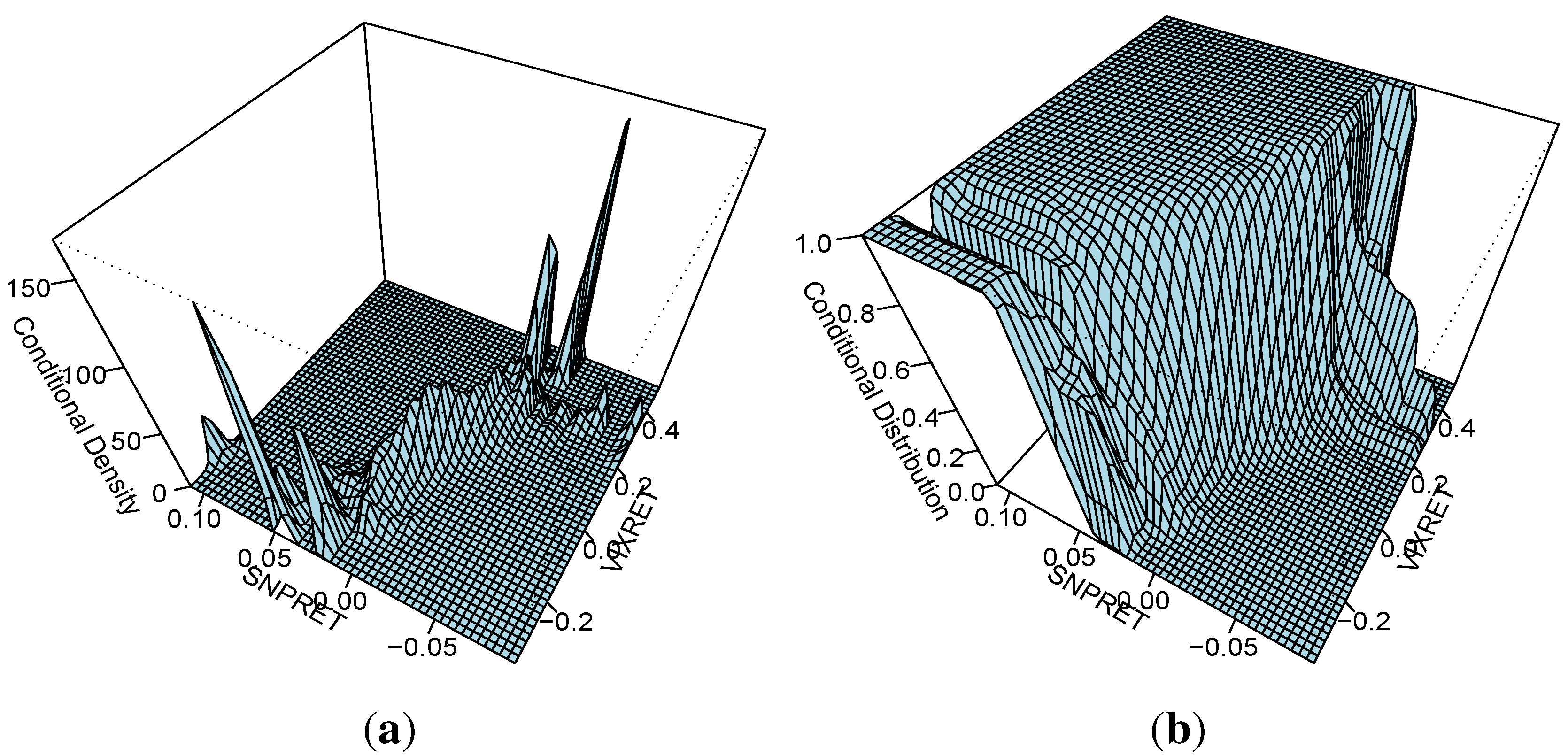
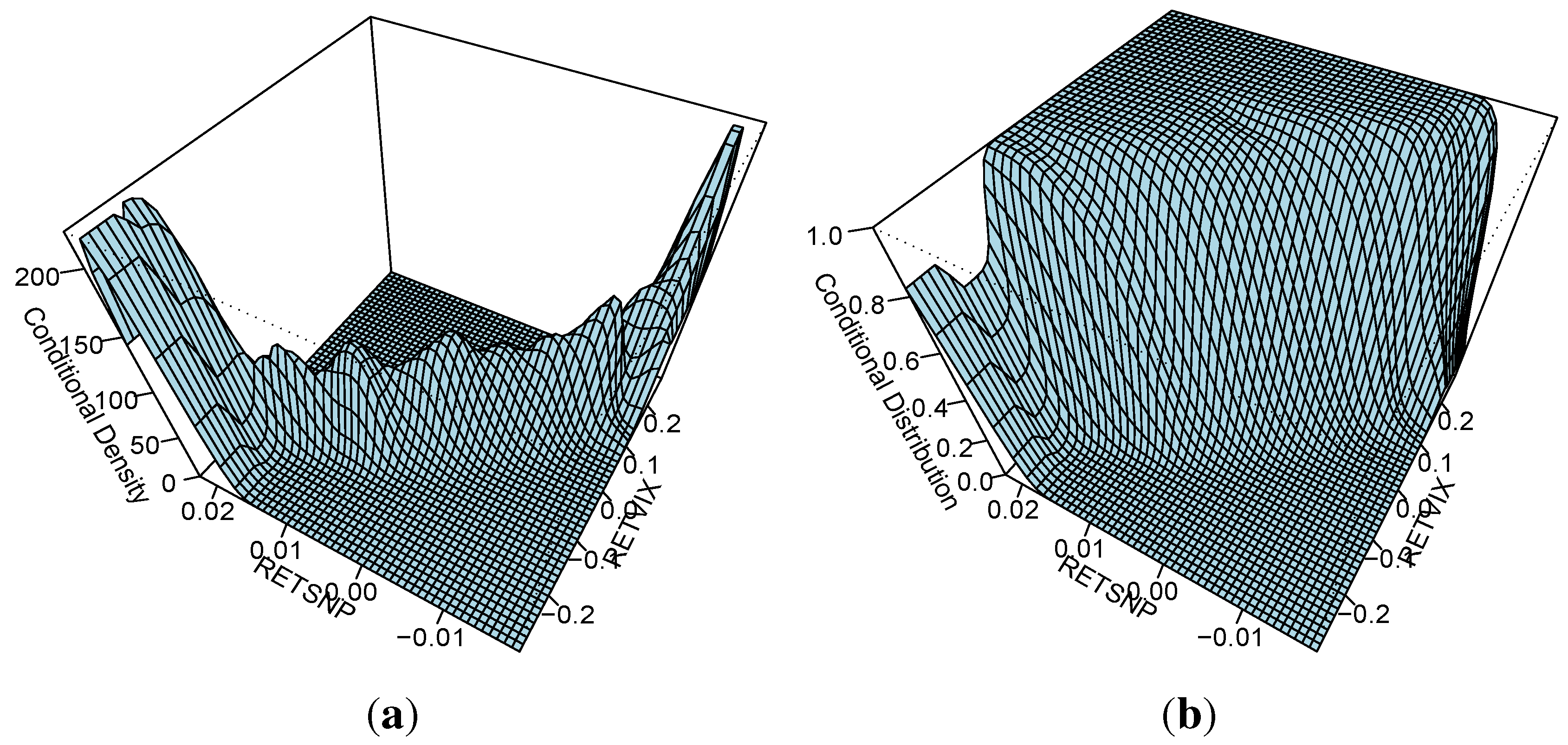
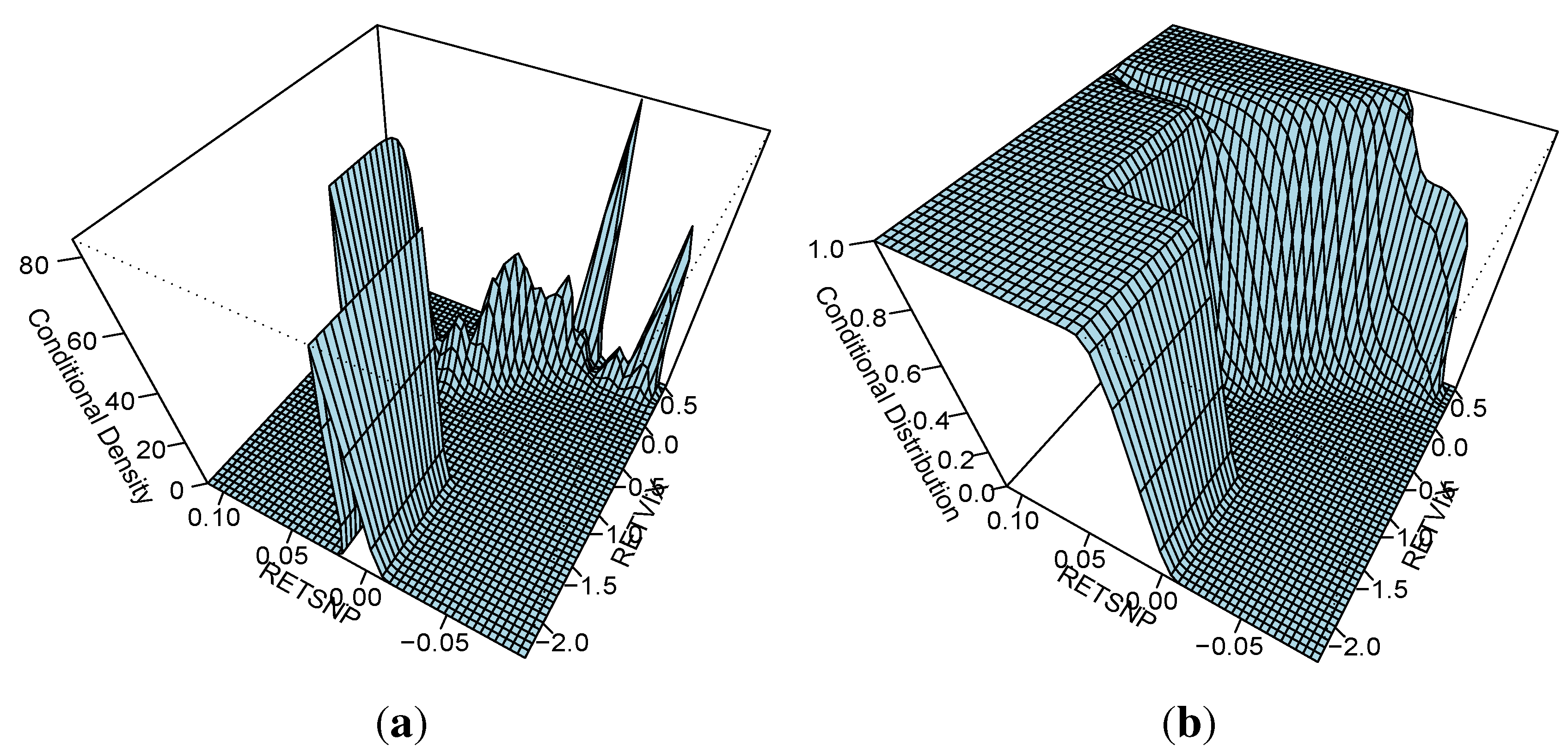
One attractive set of measures that are distribution free are based on entropy. The concept of entropy originates from physics in the 19th century; the second law of thermodynamics stating that the entropy of a system cannot decrease other way than by increasing the entropy of another system. As a consequence, the entropy of a system in isolation can only increase or remain constant over time. If the stock market is regarded as a system, then it is not an isolated system: there is a constant transfer of information between the stock market and the real economy. Thus, when information arrives from (leaves to) the real economy, then we can expect to see an increase (decrease) in the entropy of the stock market, corresponding to situations of increased (decreased) randomness.

Most often, entropy is used in one of the two main approaches, either as Shannon Entropy—in the discrete case, or as Differential Entropy—in the continuous time case. Shannon Entropy quantifies the expected value of information contained in a realization of a discrete random variable. Also, is a measure of uncertainty, or unpredictability: for a uniform discrete distribution, when all the values of the distribution have the same probability, Shannon Entropy reaches his maximum. Minimum value of Shannon Entropy corresponds to perfect predictability, while higher values of Shannon Entropy correspond to lower degrees of predictability. The entropy is a more general measure of uncertainty than the variance or the standard deviation, since the entropy depends on more characteristics of a distribution as compared to the variance and may be related to the higher moments of a distribution.

Secondly, both the entropy and the variance reflect the degree of concentration for a particular distribution, but their metric is different; while the variance measures the concentration around the mean, the entropy measures the diffuseness of the density irrespective of the location parameter. In information theory, entropy is a measure of the uncertainty associated with a random variable. The concept of entropy developed by Shannon [17], which quantifies the expected value of the information contained in a message, frequently measured in units such as bits. In this context, a ‘message’ means a specific realization of the random variable. The USA National Science Foundation workshop ([18], p. 4) pointed out that the, “Information Technology revolution that has affected Society and the world so fundamentally over the last few decades is squarely based on computation and communication, the roots of which are respectively Computer Science (CS) and Information Theory (IT)”. In [17] provided the foundation for information theory. In the late 1960s and early 1970s, there were tremendous interdisciplinary research activities from IT and CS, exemplified by the work of Kolmogorov, Chaitin, and Solomonoff [19,20,21], with the aim of establishing the algorithmic information theory. Motivated by approaching the Kolmogorov complexity algorithmically, A. Lempel (a computer scientist), and J. Ziv (an information theorist) worked together in later 1970s to develop compression algorithms that are now widely referred to as Lempel–Ziv algorithms. Today, these are a de facto standard for lossless text compression; they are used pervasively in computers, modems, and communication networks. Shannon’s entropy represents an absolute limit on the best possible lossless compression of any communication, under certain constraints: treating messages to be encoded as a sequence of independent and identically-distributed random variables Shannon’s source coding theorem shows that, in the limit, the average length of the shortest possible representation to encode the messages in a given alphabet is their entropy divided by the logarithm of the number of symbols in the target alphabet. For a random variable X with n outcomes, $\left\{x_i:i=1,.....n\right\}$, the Shannon entropy is defined as:

$$H\left(X\right)=-\sum _{i=1}^{n}p\left(x_i\right)lo{g}_{b}p\left(x_i\right)$$

(2)

where $p\left(x_i\right)$ is the probability mass function of outcome $x_i$. Usually logarithms base 2 are used when we are dealing with bits of information. We can also define the joint entropy of two random variables as follows:

$$H\left[X,Y\right]=-\sum _{x\in \chi }\sum _{y\in \gamma }Pr(x,y)lo{g}_2\left(Pr(x,y)\right).$$

(3)

The joint entropy is a measure of the uncertainty associated with a joint distribution. Similarly, the conditional entropy can be defned as:

$$H\left[X\mid Y\right]=-\sum _{x\in \chi }\sum _{y\in \gamma }Pr(x,y)lo{g}_{2}Pr(x\mid y)$$

(4)

where the conditional entropy measures the uncertainty associated with a conditional probability. Clearly, a generalized measure of uncertainty has lots of important implications across a wide number of disciplines. In the view of [22], thermodynamic entropy should be seen as an application of Shannon’s information theory. Jaynes [22] gathers various threads of modern thinking about Bayesian probability and statistical inference, develops the notion of probability theory as extended logic and contrasts the advantages of Bayesian techniques with the results of other approaches. Golan [23] provides a survey of information-theoretic methods in econometrics, to examine the connecting theme among these methods, and to provide a more detailed summary and synthesis of the sub-class of methods that treat the observed sample moments as stochastic. Within the above objectives, this review focuses on studying the interconnection between information theory, estimation, and inference. Granger, Massoumi and Racine [24] applied estimators based on this approach as a dependence metric for nonlinear processes. Pincus [25] demonstrates the utility of approximate entropy (ApEn), a model-independent measure of sequential irregularity, via several distinct applications, both empirical data and model-based. He also considers cross-ApEn, a related two-variable measure of asynchrony that provides a more robust and ubiquitous measure of bivariate correspondence than does correlation, and the resultant implications for diversification strategies and portfolio optimization. A theme further explored by Bera and Park [26]. Sims [27] discusses information theoretic approaches that have been taken in the existing economics literature to applying Shannon capacity to economic modeling, whilst both critiquing existing models and suggesting promising directions for further progress.

Usually, the variance is the central measure in the risk and uncertainty analysis in financial markets. However, the entropy measure can be used as an alternative measure of dispersion, and some authors consider that the variance should be interpreted as a measure of uncertainty with some precaution (see, e.g., [28,29]). Ebrahimi, Maasoumi and Soofi [30] examined the role of the variance and entropy in ordering distributions and random prospects, and concluded that there is no general relationship between these measures in terms of ordering distributions. They found that, under certain conditions, the ordering of the variance and entropy is similar for transformations of continuous variables, and show that the entropy depends on many more parameters of a distribution than the variance. Indeed, a Legendre series expansion shows that the entropy is related to higher-order moments of a distribution and thus, unlike the variance, could offer a better characterization of $p_X\left(x\right)$ since it uses more information about the probability distribution than the variance (see [30]).

Maasoumi and Racine [31] argue that when the empirical probability distribution is not perfectly known, then entropy constitutes an alternative measure for assessing uncertainty, predictability and also goodness-of-fit. It has been suggested that entropy represents the disorder and uncertainty of a stock market index or a particular stock return series, since entropy has the ability to capture the complexity of systems without requiring rigid assumptions that may bias the results obtained.

To estimate entropy we used the “entropy package” in the R library. Hausser and Strimmer [32], provide an explanation of how they develop their estimators: to define the Shannon entropy, they consider a categorical random variable with alphabet size p and associated cell probabilities ${\theta }_1,.....,{\theta }_p,$ with ${\theta }_k>0$ and ${\sum }_k{\theta }_k=1$. (By alphabet size the reference is to the source alphabet which consists of blocks of elementary symbols of equal size; which are typically of 8-bits in information theory applications, but in this case, are the number of categories used for estimation purposes). It is assumed that p is fixed and known and in this case Shannon entropy in natural units is given by:

$$H=-\sum _{k=1}^p{\theta }_{k}log\left({\theta }_k\right).$$

(5)

In practice the underlying probability mass function is unknown and therefore H and ${\theta }_k$ need to be estimated from observed cell counts from the sample used $y_k\ge 0$. (The index y in this case refers to the number of bins used). A commonly used estimator of entropy is the maximum likelihood estimator (ML) which is given by:

$${\widehat{H}}^{ML}=-\sum _{k=1}^p{\widehat{\theta }}_k^{ML}log\left({\widehat{\theta }}_k^{ML}\right).$$

(6)

This is formed by substituting in the ML frequency estimates

$${\widehat{\theta }}_k^{ML}=\frac{y_k}{n}$$

(7)

into Equation (5), with $n={\sum }_{k=1}^p{y}_k$ being the total number of counts.

2.1.1. Maximum Likelihood Estimation

The multinomial distribution is used to make the connection between observed counts $y_k$ and frequencies ${\theta }_k$.

$$Prob(y_1,......,y_p)=\frac{n!}{{\prod }_{k=1}^p{y}_k!}\prod _{k=1}^p{\theta }_k^{y_k}.$$

(8)

Note that ${\theta }_k>0$ otherwise the distribution is singular. By contrast there may be zero counts $y_k$. The ML estimator of ${\theta }_k$maximizes the right hand side of Equation (8) for fixed $y_k$, leading to the observed frequencies ${\widehat{\theta }}_k^{ML}=\frac{y_k}{n}$ with variances $Var\left({\widehat{\theta }}_k^{ML}\right)=\frac{1}{n}{\theta }_k(1-{\theta }_k)$ and Bias $\left({\widehat{\theta }}_k^{ML}\right)=0$ as $E\left({\widehat{\theta }}_k^{ML}\right)={\theta }_k$.

2.1.2. Miller–Madow Estimator

Even though ${\theta }_K^{ML}$ is unbiased, the plug in entropy estimator ${\widehat{\theta }}^{ML}$ is not. First order bias correction leads to:

$${\widehat{H}}^{MM}={\widehat{H}}^{ML}+\frac{m>0-1}{2n}$$

(9)

where $m>0$ is the number of cells with $y_k>0$. This is termed the Miller–Madow estimator, see [33].

2.1.3. Bayesian Estimators

Bayesian regularization of the cell counts may lead to improvements over ML estimates. The Dirichlet distribution with parameters $a_1,a_2,......,a_p$ as prior, the resulting posterior distribution is also Dirichlet with mean

$${\widehat{\theta }}_k^{Bayes}=\frac{y_k+a_k}{n+A}$$

where $A={\sum }_{k=1}^p{a}_k$. The flattening constants $a_k$ play the role of pseudo counts (compare with Equation (7)), therefore A may be interpreted as the $apriori$ sample size.

$${\widehat{H}}^{Bayes}=-\sum _{k=1}^p{\widehat{\theta }}_k^{Bayes}log\left({\widehat{\theta }}_k^{Bayes}\right).$$

(10)

2.1.4. The Chao–Shen Estimator

In [34] estimator utilizes the [35] estimator combined with the Good–Turing correction (see [36,37]), in the utilization of the empirical cell probabilities to the issue of entropy estimation. The frequency estimates after application of the Good–Turing correction are:

$${\widehat{\theta }}_k^{GT}=(1-\frac{m_1}{n}){\widehat{\theta }}_k^{ML}$$

where $m_1$ represents the number of singletons, in effect cells with $y_k=1$. If this is combined with the Horvitz–Thompson estimator the result is:

$${\widehat{H}}^{CS}=-\sum _{k=1}^p\frac{{\widehat{\theta }}_k^{GT}log{\widehat{\theta }}_k^{GT}}{(1-{(1-{\widehat{\theta }}_k^{GT})}^n}.$$

(11)

2.1.5. Mutual Information

One attraction of entropy-based measures is that they can relax the linearity assumption and capture nonlinear associations amongst variables. The starting point is to capture the mutual information between pairs of variables $MI(X,Y)$. The mutual information is the Kullback–Leibler distance from the joint probability density to the product of the marginal probability densities:

$$MI(X,Y)=E_{f(x,y)}\left\{log\frac{f(x,y)}{f\left(x\right)f\left(y\right)}\right\}.$$

(12)

The measure mutual information ($MI$) is always non-negative, symmetric, and equals zero only if X and Y are independent. In the case of normally distributed variables $MI$ is closely related to the Pearson correlation coefficient.

$$MI(X,Y)=-\frac{1}{2}log(1-{\rho }^2).$$

The entropy representations is:

$$MI(X,Y)=H\left(X\right)+H\left(Y\right)-H(X,Y).$$

(13)

This shows that $MI$ can be computed from the joint and marginal entropies of the two variables.

2.2. Some Preliminary Results

Table 4 presents some of the common methods adopted.

Table 4. Common choices for the parameters of the Dirichlet prior in the Bayesian estimators of cell frequencies, and corresponding entropy estimators.

$a_k$	Cell Frequency Prior	Entropy Estimator
0	no prior	maximum likelihood
1/2	Jeffreys prior ([38])	[39]
1	Bayes–Laplace uniform prior	[40]
1/p	Perks prior ([41])	[42]
$\sqrt{n}/p$	minmax prior ([43])

Source: [32].

Table 4. Common choices for the parameters of the Dirichlet prior in the Bayesian estimators of cell frequencies, and corresponding entropy estimators.

$a_k$	Cell Frequency Prior	Entropy Estimator
0	no prior	maximum likelihood
1/2	Jeffreys prior ([38])	[39]
1	Bayes–Laplace uniform prior	[40]
1/p	Perks prior ([41])	[42]
$\sqrt{n}/p$	minmax prior ([43])

Source: [32].

We used our returns series for S&P500 and VIX and estimated their entropy and cross-entropy. The results are shown in Table 5.

Table 5. Entropy and $MI$ statistics for S&P500 Returns and VIX Returns 1990–June 2011.

	S&P500 returns	VIX returns
Maximum Likelihood Estimate	2.1434	3.8269
Miller–Madow Estimator	2.1462	3.8367
Jeffrey’s prior	2.1598	3.8846
Bayes–Laplace	2.1747	3.9322
SG	2.1444	3.8279
Minimax	2.1983	3.8780
Chao–Shen	2.1494	3.8424
Mutual Information $MI$
$MI$ Dirichlet ( a = 0)	0.3535395
$MI$ Dirichlet ( a = 1/2)	0.3465671
$MI$ Empirical ($ML)$	0.3535395

Table 5. Entropy and $MI$ statistics for S&P500 Returns and VIX Returns 1990–June 2011.

	S&P500 returns	VIX returns
Maximum Likelihood Estimate	2.1434	3.8269
Miller–Madow Estimator	2.1462	3.8367
Jeffrey’s prior	2.1598	3.8846
Bayes–Laplace	2.1747	3.9322
SG	2.1444	3.8279
Minimax	2.1983	3.8780
Chao–Shen	2.1494	3.8424
Mutual Information $MI$
$MI$ Dirichlet ( a = 0)	0.3535395
$MI$ Dirichlet ( a = 1/2)	0.3465671
$MI$ Empirical ($ML)$	0.3535395

It can be seen in Table 5 that the different estimation methods produce very similar results. The entropy estimates for the S&P500 returns vary in a band between 2.1434 and 2.1983, whilst those for the VIX vary between 3.8269 and 3.9322. The Bayes–Laplace method gives higher entropy entropy statistics but it can be seen in Table 4 that this method has a relatively higher prior probability of unity.

2.3. Non-Parametric Estimation

Hayfield and Racine [44] (p.1) comment that: “the appeal of nonparametric methods, for applied researchers at least, lies in their ability to reveal structure in data that might be missed by classical parametric methods”. Their “NP” package available in R provides a flexible underlying the treatment of kernel methods in the presence of a mix of categorical and continuous data and lies in the use of what they call `generalized product kernels’. They develop their approach as follows: suppose you are confronted with discrete data $X^d\in S^d$ where $S^d$ denotes the support of $X^d$. If we use $x_s^d$ and $X_{is}^d$ to denote the sth component of $x^d$ and $X_i^d\in \left\{0,1,.....,c_s-1\right\}$, we define a discrete univariate kernel function

$$l^u(X_{is}^d,x_s^d,{\lambda }_s)=\left\{\begin{array}{cc}1-{\lambda }_s& if{X}_{is}^d=x_s^d\\ {\lambda }_s/(c_s-1)& if{X}_{is}^d\ne x_s^d\end{array}\right\}.$$

(14)

Note that when ${\lambda }_s=0,l(X_{is}^d,x_s^d,0)=1(X_{is}^d=x_s^d$ becomes an indicator function, and if ${\lambda }_s=(c_s-1)/c_s$ then $l(X_{is}^d=x_s^d,\frac{c_s-1}{c_s}$) = $1/c_s$ is a constant for all values of $X_{is}^d$ and $x_s^d$. The range of ${\lambda }_s$ is $\left[0,(c_s-1)/c_s\right]$. Observe that these weights sum to one. If a variable was continuous, you could use, the second order Gaussian kernel, namely

$$w(x^c,X_i^c,h)=\frac{1}{\sqrt{2\pi }}exp\left\{-\frac{1}{2}{\left(\frac{X_i^c-x^c}{h}\right)}^2\right\}.$$

(15)

Observe that these weights integrate to 1.

2.3.1. Kernel Estimation of a Conditional Quantile

Once we can estimate conditional CDFs such as those shown in Figure 5, we can then estimate conditional quantiles, (see the discussion in [45], p. 24–31. Regression estimates involve modeling the conditional mean but Racine [45] suggests the conditional quantile function provides a more comprehensive picture of the conditional distribution of a dependent variable than the conditional mean function).

Figure 5. Nonparametric conditional PDF and CDF estimates of the joint distribution of S&P500 returns and VIX returns 1990-June 2011. (a) PDF; (b) CDF.

Figure 5. Nonparametric conditional PDF and CDF estimates of the joint distribution of S&P500 returns and VIX returns 1990-June 2011. (a) PDF; (b) CDF.

That is, having estimated the conditional CDF we simply invert it at the desired quantile as described in Equation (15). A conditional α th quantile of a conditional distribution function $F(·\mid x)$ is defined by $(\alpha \in (0,1\left)\right)$

$$q_{\alpha }\left(x\right)=inf\left\{y:F(y\mid x)\ge \alpha \right\}=F^{-1}(\alpha \mid x),$$

(16)

or equivalently $F(q_{\alpha }\left(x\right)\mid x)=\alpha .$ The conditional quantile function $q_{\alpha }\left(x\right)$ can be directly estimated by inverting the previously estimated conditional CDF function. In effect:

$$q_{\alpha }\left(x\right)=inf\left\{y:\widehat{F}(y\mid x)\ge \alpha \right\}\equiv {\widehat{F}}^{-1}(\alpha \mid x).$$

(17)

2.3.2. Testing the Equality of Univariate Densities

Massoumi and Racine [31] suggest a metric entropy which is useful for testing for the equality of densities for two univariate random variables X and Y. They compute the nonparametric metric entropy (normalised Hellinger of Granger [24]). This tests the null of equality of two univariate density functions. For continuous variables they suggest the construction of:

$$\begin{array}{ccc}\hfill S_p& =& \frac{1}{2}\int {(f_1^{1/2}-f_2^{1/2})}^{2}dx\hfill \\ & =& \frac{1}{2}\int {\left(1-\frac{f_2^{1/2}}{f_1^{1/2}}\right)}^{2}d{F}_1\left(x\right)\hfill \end{array}$$

where $f_1=f\left(x\right)$ and $f_2=f\left(y\right)$ are the marginal densities of the random variables X and Y. If X and Y are discrete or categorical, then the integration can be replaced by summing over all possible outcomes.

3. Main Results

3.1. Entropy Metrics

We focus our attention on a time frame during which the current VIX has been in operation. We obtained our data from SIRCA’s TRTH data and obtained daily closing prices for the VIX beginning in March 2005 and running through until May 2012. The data was divided into roughly two year periods as we wanted to explore how these measures varied during times of crisis. Table 5 presents the entropy measures for our two daily continuously compounded return series; S&P500 and VIX for four roughly one and a half to two year blocks running from: 9th March 2005 until 29th December 2006, 3rd January 2007 to 31st December 2008, 2nd January 2009 to 31st December 2010, and 3rd January 2011 to 1st May 2012.

Table 6. Entropy measures S&P500 continuously compounded daily returns March 2005 to May 2012.

	S&P500 2005–2006	S&P500 2007–2008	S&P500 2009–2010	S&P500 2011–2012
Maximum Likelihood Estimate	1.6518	2.4165	2.2611	2.1859
Miller–Madow Estimator	1.6596	2.4454	2.2790	2.2211
Jeffrey’s prior	1.6610	2.5364	2.2956	2.2516
Bayes–Laplace	1.6698	2.6299	2.3262	2.3051
SG	1.6542	2.4243	2.2649	2.1935
Minimax	1.6967	2.545	2.331	2.2920
Chao–Shen	1.6527	2.4781	2.2809	2.2282
Mutual Information $MI$ S&P500 and VIX
$MI$ Dirichlet ( a = 0)	0.09489	0.1941	0.1927	0.2055
$MI$ Dirichlet ( a = 1/2)	0.08485	0.1693	0.1702	0.1746
$MI$ Empirical ($ML)$	0.09489	0.1941	0.1927	0.2055

Table 6. Entropy measures S&P500 continuously compounded daily returns March 2005 to May 2012.

	S&P500 2005–2006	S&P500 2007–2008	S&P500 2009–2010	S&P500 2011–2012
Maximum Likelihood Estimate	1.6518	2.4165	2.2611	2.1859
Miller–Madow Estimator	1.6596	2.4454	2.2790	2.2211
Jeffrey’s prior	1.6610	2.5364	2.2956	2.2516
Bayes–Laplace	1.6698	2.6299	2.3262	2.3051
SG	1.6542	2.4243	2.2649	2.1935
Minimax	1.6967	2.545	2.331	2.2920
Chao–Shen	1.6527	2.4781	2.2809	2.2282
Mutual Information $MI$ S&P500 and VIX
$MI$ Dirichlet ( a = 0)	0.09489	0.1941	0.1927	0.2055
$MI$ Dirichlet ( a = 1/2)	0.08485	0.1693	0.1702	0.1746
$MI$ Empirical ($ML)$	0.09489	0.1941	0.1927	0.2055

The results in Table 6 and Table 7 are consistent and intuitive. Entropy measures capture changes in uncertainty, and clearly for both the S&P500 and the VIX the maximum uncertainty, in terms of entropy measures, the highest minimum estimates of 2.42 for the S&P500 continuously compounded daily returns, or 4.01 for the VIX continuously compounded daily returns were recorded in the two year interval 2007–2008. Given that this captures the start of the Global Financial Crisis (GFC), this is not surprising. The Mutual Information (MI) measure results are a bit more surprising. Mutual information measures the information that X and Y share: it measures how much knowing one of these variables reduces uncertainty about the other. The measure at the foot of Table 6 suggests that the amount of information revealed by the VIX’s continuously compounded daily returns about the S&P500 continuously compounded returns increases over the two year time frames examined and records its highest levels on two metrics of over 0.20 in the period 2011–2012.

The entropy measures for VIX are shown in Table 7.

Table 7. Entropy measures VIX continuously compounded daily returns March 2005 to May 2012.

	VIX 2005–2006	VIX 2007–2008	VIX 2009–2010	VIX 2011–2012
Maximum Likelihood Estimate	3.6441	4.0114	3.7744	3.8723
Miller–Madow Estimator	3.7045	4.0911	3.8421	3.9669
Jeffrey’s prior	3.9220	5.3321	4.0743	4.2843
Bayes–Laplace	4.0811	5.7334	4.2444	4.4751
SG	3.6541	4.0278	3.7835	3.8861
Minimax	3.7787	4.2524	3.9054	4.0306
Chao–Shen	3.7086	4.1006	3.8539	3.9573

Table 7. Entropy measures VIX continuously compounded daily returns March 2005 to May 2012.

	VIX 2005–2006	VIX 2007–2008	VIX 2009–2010	VIX 2011–2012
Maximum Likelihood Estimate	3.6441	4.0114	3.7744	3.8723
Miller–Madow Estimator	3.7045	4.0911	3.8421	3.9669
Jeffrey’s prior	3.9220	5.3321	4.0743	4.2843
Bayes–Laplace	4.0811	5.7334	4.2444	4.4751
SG	3.6541	4.0278	3.7835	3.8861
Minimax	3.7787	4.2524	3.9054	4.0306
Chao–Shen	3.7086	4.1006	3.8539	3.9573

This leads to consideration of the nature of the two probability density functions for the two return series. We have generated the non parametric conditional PDF and CDF conditioning the S&P500 returns on the VIX returns for our roughly two-year sample intervals. We suspect that the relationship may not remain constant through time. The results are shown in Figure 6.

Figure 6. Conditional Density Plots PDF and CDF for S&P500 and VIX returns 2005–2006 for our sample intervals. (a) PDF 2005–2006; (b) CDF 2005–2006.

Figure 6. Conditional Density Plots PDF and CDF for S&P500 and VIX returns 2005–2006 for our sample intervals. (a) PDF 2005–2006; (b) CDF 2005–2006.

3.2. Non-Parametric Conditional PDF and CDF Estimation

Figure 7. Conditional Density Plots PDF and CDF for S&P500 and VIX returns 2005-2006 for our sample intervals. (a) PDF 2007–2008; (b) CDF 2007–2008.

Figure 7. Conditional Density Plots PDF and CDF for S&P500 and VIX returns 2005-2006 for our sample intervals. (a) PDF 2007–2008; (b) CDF 2007–2008.

Figure 8. Conditional Density Plots PDF and CDF for S&P500 and VIX returns 2009-2010 for our sample interval. (a) PDF 2009–2010; (b) CDF 2009–2010.

Figure 8. Conditional Density Plots PDF and CDF for S&P500 and VIX returns 2009-2010 for our sample interval. (a) PDF 2009–2010; (b) CDF 2009–2010.

Figure 9. Conditional Density Plots PDF and CDF for S&P500 and VIX returns 2011-2012 for our sample interval. (a) PDF 2011–2012; (b) CDF 2011–2012.

Figure 9. Conditional Density Plots PDF and CDF for S&P500 and VIX returns 2011-2012 for our sample interval. (a) PDF 2011–2012; (b) CDF 2011–2012.

3.3. Quantile Regression Analysis of Hedge Ratios

The relationship between the S&P500 and the VIX can be further explored by application of quantile regression. This will help to shed light on whether hedging ratios are likely to be constant across the two distributions. Quantile regression is modeled as an extension of classical OLS [46], in quantile regression the estimation of conditional mean as estimated by OLS is extended to similar estimation of an ensemble of models of various conditional quantile functions for a data distribution. In this fashion quantile regression can better quantify the conditional distribution of $\left(Y\right|X)$. The central special case is the median regression estimator that minimizes a sum of absolute errors. We get the estimates of remaining conditional quantile functions by minimizing an asymmetrically weighted sum of absolute errors, here weights are the function of the quantile of interest. This makes quantile regression a robust technique even in presence of outliers. Taken together the ensemble of estimated conditional quantile functions of $\left(Y\right|X)$ offers a much more complete view of the effect of covariates on the location, scale and shape of the distribution of the response variable.

For parameter estimation in quantile regression, quantiles as proposed by Koenker and Bassett [46] can be defined through an optimization problem. The median quantile (0.5%) in quantile regression is defined through the problem of minimizing the sum of absolute residuals. The symmetrical piecewise linear absolute value function assures the same number of observations above and below the median of the distribution. The other quantile values can be obtained by minimizing a sum of asymmetrically weighted absolute residuals, giving different weights to positive and negative residuals. Proceeding with:

$$min\xi \epsilon R\sum {\rho }_{\tau }(y_i-\xi )$$

(18)

where ${\rho }_{\tau }(\cdot )$ is the tilted absolute value function. Taking the directional derivatives of the objective function with respect to ξ from left to right, shows that this problem yields the sample quantile as its solution. To obtain an estimate of the conditional median function, the scalar ξ in the first equation is replaced by the parametric function $\xi (x_t,\beta )$ and τ is set to 1/2 . The estimates of the other conditional quantile functions are obtained by replacing absolute values by ${\rho }_{\tau }(\cdot )$ and solving

$$mi{n}_{\mu \epsilon R^p}\sum {\rho }_{\tau }(y_i-\xi (x_i,\beta )).$$

(19)

The resulting minimization problem, when $\xi (x,\beta )$ is formulated as a linear function of parameters, and can be estimated very efficiently by linear programming methods. The slope coefficients from the results of quantile regression of the daily continuously compounded S&P 500 returns and the daily continuously compounded VIX returns are shown in Figure 10 and Figure 11 All the slope coefficients are significant at a 1% level and all are negative, confirming the utility of the conceptual employment of VIX returns as a hedge against movements in S&P 500 returns. In addition, the quantile regression slope coefficients vary considerably across the deciles, and also the nature of this variation is not consistent. the first period hedge ratios become less negative by the decile, whilst in the second period the reverse occurs and they become more negative as they progress across the deciles. In the third period they continually increase, whilst in the fourth they steadily increase until the 7th decile and then become progressively more negative. These results are suggestive of the difficulty of setting up precise hedges incorporating volatility changes. In practice it is more difficult than this suggests, as instruments written against the VIX, options or futures, have to be used in practice.

Figure 10. Quantile regression slope coefficients of S&P 500 daily returns for sample sub-periods regressed in daily continuously compounded VIX returns, sub-samples 2005–2006 and 2007–2008. (a) Quantile regression slope coefficients by decile 2005–2006 with error bands; (b) Quantile regression slope coefficients by decile 2007–2008 with error bands.

Figure 10. Quantile regression slope coefficients of S&P 500 daily returns for sample sub-periods regressed in daily continuously compounded VIX returns, sub-samples 2005–2006 and 2007–2008. (a) Quantile regression slope coefficients by decile 2005–2006 with error bands; (b) Quantile regression slope coefficients by decile 2007–2008 with error bands.

Figure 11. Quantile regression slope coefficients of S&P500 daily returns for sample sub-periods regressed in daily continuously compounded VIX returns, sub-samples 2009–2010 and 2011–2012. (a) Quantile regression slope coefficients by decile 2009–2010 with error bands; (b) Quantile regression slope coefficients by decile 2011–2012 with error bands.

Figure 11. Quantile regression slope coefficients of S&P500 daily returns for sample sub-periods regressed in daily continuously compounded VIX returns, sub-samples 2009–2010 and 2011–2012. (a) Quantile regression slope coefficients by decile 2009–2010 with error bands; (b) Quantile regression slope coefficients by decile 2011–2012 with error bands.

3.4. Non-Parametric Tests of Density Equalities

Our final set of tests feature an a non-parametric analysis of the equivalence of the density functions of our two sets of return distributions derived from the S&P 500 and the VIX. We apply the Massoumi and Racine [31] metric entropy test of the equality of the densities of two random variables, in this case, the continuously compounded daily S&P500 returns and the daily continuously compounded VIX returns for our four subsample periods from 2005 to 2012. The bootstrap test is conducted by sampling with replacement from the pooled empirical distribution of the return series. We also conduct a non-parametric test of the symmetry of the two distributions of returns. This is a non-parametric metric entropy discussed in [47] which tests the null of symmetry using the densities/probabilities of the data series and rotated data series. Bootstrapping is conducted by resampling from the empirical distribution of the pooled data and rotated data. The results are shown in Table 8 and Table 9.

Table 8. Entropy density equality tests for sub-samples 2005–2006, 2007–2008, 2009–2010, and 2011–2012 for daily continuously compounded S&P 500 returns and VIX returns.

	2005–2006	2007–2008	2009–2010	2011–2012
Consistent Univariate Entropy Density Equality Test
Test Statistic ‘Srho’	0.4660	0.3017	0.3219	0.3817
Probability	2.22e-16 ***	2.22e-16 ***	2.22e-16 ***	2.22e-16 ***

*** Significant at 1% level.

Table 8. Entropy density equality tests for sub-samples 2005–2006, 2007–2008, 2009–2010, and 2011–2012 for daily continuously compounded S&P 500 returns and VIX returns.

	2005–2006	2007–2008	2009–2010	2011–2012
Consistent Univariate Entropy Density Equality Test
Test Statistic ‘Srho’	0.4660	0.3017	0.3219	0.3817
Probability	2.22e-16 ***	2.22e-16 ***	2.22e-16 ***	2.22e-16 ***

*** Significant at 1% level.

The results of the entropy based density equality tests shown in Table 8 clearly reject the null that the distributions of the daily returns on the S&P 500 series and the VIX series in our four subsample periods are drawn from the same distribution and all the results are highly significant at the 1% level. The entropy based tests of asymmetry results in Table 9 also reject the null of symmetry at the 1% level in the cases of the S&P 500 in the period 2007–2008, and the VIX in 2009–2010, and 2011–2012. These results also support our examination of the conditional density functions of the two series and Figure 6, Figure 7, Figure 8 to Figure 9 which strongly suggested the existence of assymetry and non-equality of the two sets of return distributions in our four sub sample periods.

Table 9. Entropy density asymmetry tests sub-samples 2005–2006, 2007–2008, 2009–2010, and 2011–2012 for daily continuously compounded S&P 500 returns and VIX returns.

	2005–2006	2007–2008	2009–2010	2011–2012
Consistent entropy asymmetry test
S&P 500 Test Statistic ‘Srho’	0.00419	0.034547	0.01239	0.01904
Probability	0.52525	0.0 ***	0.19191	0.09090
VIX Test Statistic ‘Srho’	0.00923	0.01278	0.02485	0.03018
Probability	0.1818	0.15151	0.0 ***	0.0 ***

*** Significant at 1% level.

Table 9. Entropy density asymmetry tests sub-samples 2005–2006, 2007–2008, 2009–2010, and 2011–2012 for daily continuously compounded S&P 500 returns and VIX returns.

	2005–2006	2007–2008	2009–2010	2011–2012
Consistent entropy asymmetry test
S&P 500 Test Statistic ‘Srho’	0.00419	0.034547	0.01239	0.01904
Probability	0.52525	0.0 ***	0.19191	0.09090
VIX Test Statistic ‘Srho’	0.00923	0.01278	0.02485	0.03018
Probability	0.1818	0.15151	0.0 ***	0.0 ***

*** Significant at 1% level.

4. Conclusions

We have examined the relationship between the S&P 500 daily continuously compounded return series and a similar series for the VIX in terms of a long sample drawn from the CBOE website running from 1990 to mid 2011 and a set of returns from SIRCA’s TRTH datasets running from March 2005 to-date which we divided into four roughly equivalent sub-samples and subjected to a series of non-parametric based tests utilizing entropy based metrics. These suggested that the PDFs and CDFs of these two return distributions change shape in various subsample periods. The entropy and MI statistics suggest that the degree of uncertainty attached to these distributions changes through time and using the S&P 500 return as the dependent variable, the amount of information obtained from the VIX also changes with time, though it increased in the most recent period from 2011 to 2012. The entropy based non parametric tests of the equivalence of the two distributions and their symmetry strongly reject their respective nulls in the case of the first test and in certain periods for the second test.

The implication of these non-parametric tests is that the relationship between the S&P 500 and the VIX is complex and subject to change in different time periods. This implies that portfolio risk-hedging using the two series will be complex and difficult to calibrate. This is compounded by the fact that the VIX is not a cash instrument and derivates written against the VIX such as options and futures have to be utilized for practical hedging purposes and therefore add a second layer of complexity. The analysis of which will be the subject of a companion paper.

References

1. K. Demeterfi, E. Derman, M. Kamal, and J. Zou. “More than you ever wanted to know about volatility swaps.” Quantative Strategies Research Notes. New York, NY, USA: Goldman Sachs, 1999. available online at http://www.emanuelderman.com/writing/entry/more-than-you-ever-wanted-to-know-about-volatility-swaps-the-journal-of-der (accessed on 18 October 2013).
2. C.-L. Chang, J.-A. Jiminez-Martin, M. McAleer, and T. Perez-Amaral. “The rise and fall of S&P500 variance futures.” North Am. J. Econ. Financ. 25 (2013): 151–167. [Google Scholar]
3. A. Sepp. “VIX Option Pricing in a Jump-Diffusion Model.” Risk Magazine, April 2008, 84–89. [Google Scholar]
4. M. Caporin, and M. McAleer. “Do we really need both BEKK and DCC? A tale of two multivariate GARCH models.” J. Econ. Surv. 26 (2012): 736–751. [Google Scholar] [CrossRef]
5. M. Brenner, E.Y. Ou, and J.E. Zhang. “Hedging volatility risk.” J. Bank. Financ. 30 (2006): 811–821. [Google Scholar] [CrossRef]
6. B. Huskaj. A value-at-risk analysis of VIX futures: Long memory, heavy tails, and asymmetry, 2009. Working Paper; Rochester, NY, USA: Social Science Research Network, 2009. [Google Scholar] [CrossRef]
7. M. McAleer, and C. Wiphatthanananthakul. “A simple expected volatility (SEV) index: Application to SET50 index options.” Math. Comput. Simul. 80 (2010): 2079–2090. [Google Scholar] [CrossRef]
8. I. Ishida, M. McAleer, and K. Oya. “Estimating the leverage parameter of continuous-time stochastic volatility models using high frequency S&P500 and VIX.” Manag. Financ. 37 (2011): 1048–1067. [Google Scholar]
9. C. Alexander, and D. Korovilas. The Hazards of Volatility Diversification, the University of Reading. ICMA Centre Discussion Papers in Finance DP2011-04; Reading, UK: ICMA, 2011. [Google Scholar]
10. B. Lui, and S. Dash. “Volatility ETFs and ETNs.” J. Trading 7 (2012): 43–48. [Google Scholar]
11. Available online at: http://www.cboe.com/micro/VIX/vixintro.aspx (accessed on 1 October 2013).
12. L. Edrington. “The hedging performance of the new futures markets.” J. Financ. 34 (1979): 157–170. [Google Scholar] [CrossRef]
13. R.F. Engle, and C.W.J. Granger. “Co-integration and error correction: representation, estimation and testing.” Econometrica 55 (1987): 251–276. [Google Scholar] [CrossRef]
14. C. Alexander. “Optimal hedging using cointegration.” Philos. Trans. R. Soc. Lond. A 357 (1999): 2039–2058. [Google Scholar] [CrossRef]
15. R.E. Whaley. “Understanding the VIX.” J. Portf. Manag. 35 (2009): 98–105. [Google Scholar] [CrossRef]
16. H.C. Thode Jr. Testing for Normality. New York, NY, USA: Marcel Dekker, 2002. [Google Scholar]
17. C.E. Shannon. “A mathematical theory of communication.” Bell Syst. Tech. J. 27 (1948): 623–656. [Google Scholar] [CrossRef]
18. National Science Foundation. Report of the National Science Foundation Workshop on Information Theory and Computer Science Interface, Workshop, Chicago, IL, USA, 17–18 October 2003.
19. A.N. Kolmogorov. “Three approaches to the quantitative definition of information.” Probl. Inf. Transm. 1 (1965): 1–7. [Google Scholar] [CrossRef]
20. G.J. Chaitin. “On the simplicity and speed of programs for computing infinite sets of natural numbers.” J. ACM 16 (1969): 407–422. [Google Scholar] [CrossRef]
21. R. Solomonoff. A Preliminary Report on a General Theory of Inductive Inference. Report V-131; Cambridge, MA, USA: Zator Co., 1960. [Google Scholar]
22. E.T. Jaynes. Probability Theory: The Logic of Science. Cambridge, UK: Cambridge University Press, 2003, ISBN 0-521- 59271-2. [Google Scholar]
23. A. Golan. “Information and entropy econometrics—Editor’s view.” J. Econom. 107 (2002): 1–15. [Google Scholar] [CrossRef]
24. C. Granger, E. Maasoumi, and J. Racine. “A dependence metric for possibly nonlinear time series.” J. Time Ser. Anal. 25 (2004): 649–669. [Google Scholar] [CrossRef]
25. S. Pincus. “Approximate entropy as an irregularity measure for financial data.” Econom. Rev. 27 (2008): 329–362. [Google Scholar] [CrossRef]
26. A.K. Bera, and S.Y. Park. “Optimal portfolio diversification using the maximum entropy principle.” Econom. Rev. 27 (2008): 484–512. [Google Scholar] [CrossRef]
27. C.A. Sims. Rational Inattention: A Research Agenda. Discussion Paper Series 1: Economic Studies No 34/2005. Frankfurt-am-Main, Germany: Deutsche Bundesbank, 2005. [Google Scholar]
28. E. Maasoumi. “A compendium to information theory in economics and econometrics.” Econom. Rev. 12 (1993): 137–181. [Google Scholar] [CrossRef]
29. E. Soofi. “Information Theoretic Regression Methods.” In Advances in Econometrics - Applying Maximum Entropy to Econometric Problems. Edited by T. Fomby and R. Carter Hill. London, UK: Jai Press Inc., 1997, Volume 12. [Google Scholar]
30. N. Ebrahimi, E. Maasoumi, and E. Soofi. “Ordering univariate distributions by entropy and variance.” J. Econom. 90 (1999): 317–336. [Google Scholar] [CrossRef]
31. E. Maasoumi, and J.S. Racine. “Entropy and predictability of stock market returns.” J. Econom. 107 (2002): 291–312. [Google Scholar] [CrossRef]
32. J. Hausser, and K. Strimmer. “Entropy inference and the James-Stein estimator, with application to nonlinear gene association networks.” J. Mach. Learn. Res. 10 (2009): 1469–1484. [Google Scholar]
33. G.A. Miller. “Note on the Bias of Information Estimates.” In Information Theory in Psychology II-B. Edited by H. Quastler. Glencoe, IL, USA: Free Press, 1955, pp. 95–100. [Google Scholar]
34. A. Chao, and T.J. Shen. “Nonparametric estimation of Shannon’s index of diversity when there are unseen species.” Environ. Ecol. Stat. 10 (2003): 429–443. [Google Scholar] [CrossRef]
35. D.G. Horvitz, and D.J. Thompson. “A generalization of sampling without replacement from a finite universe.” J. Am. Stat. Assoc. 47 (1953): 663–685. [Google Scholar] [CrossRef]
36. I.J. Good. “The population frequencies of species and the estimation of population parameters.” Biometrika 40 (1953): 237–264. [Google Scholar] [CrossRef]
37. A. Orlitsky, N.P. Santhanam, and J. Zhang. “Always good Turing: asymptotically optimal probability estimation.” Science 302 (2003): 427–431. [Google Scholar] [CrossRef] [PubMed]
38. H. Jeffreys. “An invariant form for the prior probability in estimation problems.” Proc. Royal. Soc. Lond. A 186 (1946): 453–461. [Google Scholar] [CrossRef]
39. R.E. Krichevsky, and V.K. Trofimov. “The performance of universal encoding.” IEEE Trans. Inf. Theory 27 (1981): 199–207. [Google Scholar] [CrossRef]
40. D. Holste, I. Gro�e, and H. Herzel. “Bayes’ estimators of generalized entropies.” J. Phys. A 31 (1998): 2551–2566. [Google Scholar] [CrossRef]
41. W. Perks. “Some observations on inverse probability including a new indifference rule.” J. Inst. Actuar. 73 (1947): 285–334. [Google Scholar]
42. T. Schurmann, and P. Grassberger. “Entropy estimation of symbol sequences.” Chaos 6 (1996): 414–427. [Google Scholar] [CrossRef] [PubMed]
43. S. Trybula. “Some problems of simultaneous minimax estimatio.” Ann. Math. Stat. 29 (1958): 245–253. [Google Scholar] [CrossRef]
44. T. Hayfield, and J.S. Racine. “Nonparametric econometrics: The np package.” J. Stat. Softw. 27 (2008): 1–32. [Google Scholar] [CrossRef]
45. J.S. Racine. Nonparametric Econometrics: A Primer. Hanover, MA, USA: Now Publishers Inc., 2008, Volume 3, pp. 1–88. [Google Scholar]
46. R.W. Koenker, and G. Bassett Jr. “Regression quantiles.” Econometrica 1 (1978): 33–50. [Google Scholar] [CrossRef]
47. E. Maasoumi, and J.S. Racine. “Robust Entropy-Based Test of Asymmetry for Discrete and Continuous Processes.” Econom. Rev. 28 (2009): 246–261. [Google Scholar] [CrossRef]