Dynamic Connectedness of Geopolitical Risk, Brent Crude Oil Price Changes, Gold Returns, the U.S. Dollar Index Returns, and the Thai Stock Market Returns: Evidence from a Bayesian TVC-VAR Approach

Abstract

This study examines the dynamic transmission of geopolitical risk across Brent crude oil, gold, the U.S. Dollar Index, and the Thai stock market using a Bayesian time-varying coefficient vector autoregressive (TVC-VAR) framework. Using monthly data from January 1990 to December 2025, the analysis combines time-varying impulse responses, generalized forecast error variance decomposition, dynamic connectedness measures, and network analysis. The results show substantial time variation in spillover intensity and direction. On average, Brent crude oil is the strongest net transmitter, gold has a smaller positive net position, and the U.S. Dollar Index and the Thai stock market are net receivers. Episode-specific point estimates indicate changes in transmitter-receiver roles and bilateral channels, but bootstrap sensitivity analysis shows that several apparent role changes are not statistically distinguishable once uncertainty is considered. The evidence therefore supports a dynamic, reconfigurable connectedness structure while cautioning against causal, safe-haven, or portfolio-performance interpretations that are not directly tested in this study. The findings are relevant to financial-risk monitoring and macro-financial surveillance under changing geopolitical conditions.

1. Introduction

International financial markets have become increasingly interconnected through global trade, cross-border capital flows, and rapid information transmission. In this environment, geopolitical risk (GPR) has emerged as an important source of uncertainty because wars, military conflicts, terrorism, sanctions, and geopolitical tensions can affect commodity prices, exchange rates, capital flows, and equity markets simultaneously. Major geopolitical and financial episodes have demonstrated that such disturbances can propagate across markets and alter investor expectations and risk perceptions (Caldara & Iacoviello, 2022). Unlike conventional macroeconomic shocks, geopolitical shocks are often difficult to anticipate and may generate rapidly changing cross-market responses.

The transmission of geopolitical risk is particularly relevant for crude oil, gold, the U.S. Dollar Index (DXY), and equity markets because these markets are closely linked through energy costs, inflation expectations, international capital flows, and portfolio allocation. Geopolitical tensions can disrupt oil production and transportation, while gold may attract investors seeking protection during periods of heightened uncertainty. The U.S. dollar provides an additional transmission channel because of its international reserve and commodity-pricing roles. These linkages suggest that geopolitical risk should be examined as a cross-market phenomenon rather than through isolated bilateral relationships (Hamilton, 2009; Baur & Lucey, 2010; Reboredo, 2012; Chen et al., 2024).

This issue is particularly relevant for Thailand as an emerging economy integrated into international commodity, trade, and financial markets. External movements in energy prices, exchange rates, and global capital flows can influence domestic financial conditions and the Thai stock market. Recent studies document that financial connectedness can vary substantially under periods of heightened uncertainty, while evidence for emerging markets remains comparatively limited (Chen et al., 2024; Sari et al., 2026). More recent research also emphasizes the value of dynamic financial-network approaches for identifying changes in transmission structures over time (Bouzguenda & Jarboui, 2025).

Despite this growing literature, an important question remains: do the magnitude and direction of geopolitical-risk transmission remain stable across different geopolitical and financial regimes? Existing studies often examine bilateral relationships or employ conventional VAR and rolling-window approaches. While these approaches provide useful evidence, they may not fully capture continuously evolving transmission mechanisms or changes in the roles of individual markets. Moreover, relatively limited evidence jointly examines geopolitical risk, oil, gold, the U.S. dollar, and an emerging stock market within a unified time-varying framework, particularly for Thailand. Importantly, similar levels of aggregate connectedness may arise from substantially different transmission structures across periods of stress.

1.1. Research Questions and Objectives

This study addresses four research questions: (1) Do geopolitical-risk shocks generate time-varying responses in Brent crude oil, gold, the U.S. Dollar Index, and the Thai stock market? (2) How does cross-market connectedness evolve over time and across major periods of global uncertainty? (3) Do the four financial markets change their roles as net transmitters and receivers across major geopolitical, financial, and global-risk episodes? (4) Do dominant bilateral spillover channels change in magnitude or direction across these episodes?

The main objective is to examine the time-varying transmission of geopolitical risk across Brent crude oil, gold, the U.S. Dollar Index, and the Thai stock market and to identify how the magnitude and direction of spillovers change across major geopolitical, financial, and global-risk episodes. The specific objectives are: (1) to examine the dynamic responses of the four financial markets to geopolitical-risk shocks; (2) to measure the evolution and magnitude of cross-market connectedness; (3) to identify time-varying net transmitters and receivers of shocks; and (4) to identify dominant bilateral transmission channels across major episodes.

Accordingly, four hypotheses are examined: H1: Geopolitical-risk shocks generate time-varying responses in Brent crude oil, gold, the U.S. Dollar Index, and the Thai stock market. H2: Cross-market connectedness among the four financial markets varies over time and is elevated during major periods of global uncertainty. H3: The roles of the four financial markets as net transmitters and receivers are time-varying and differ across major geopolitical, financial, and global-risk episodes. H4: Bilateral spillover channels among the four financial markets are asymmetric and change across major risk episodes.

1.2. Contributions of the Study

This study contributes to the literature in three ways. First, it provides an integrated examination of geopolitical-risk transmission across commodity, foreign-exchange, and equity markets within an emerging-market setting. Second, it applies a Bayesian time-varying framework to capture changes in spillover intensity and market roles rather than imposing constant relationships over the full sample period. Third, it combines directional and pairwise connectedness with network analysis to identify changes in the structure of shock transmission across different episodes. The empirical evidence therefore provides a more detailed understanding of how geopolitical uncertainty propagates through interconnected financial markets and offers implications for financial risk management and macro-financial policy in Thailand.

2. Literature Review

2.1. Geopolitical Risk and Oil Prices

Geopolitical risk is closely linked to crude oil because wars, sanctions, supply disruptions, and transportation risks can alter expected energy availability and production costs. Oil-price responses may therefore reflect both physical supply concerns and changing expectations about global activity (Hamilton, 2009; Caldara & Iacoviello, 2022).

Recent evidence further indicates that oil-market responses to geopolitical uncertainty are not constant over time. Their magnitude can depend on the nature of the episode and prevailing financial conditions, motivating a time-varying framework rather than a single full-sample relationship (Caldara & Iacoviello, 2022; Chen et al., 2024).

These considerations make Brent crude oil a central market in the present analysis and provide an economic basis for examining both its response to GPR shocks and its changing role in cross-market connectedness.

2.2. Geopolitical Risk and Commodity Prices

Commodity markets can respond differently to geopolitical uncertainty. In contrast to oil, gold is often associated with defensive demand during periods of heightened uncertainty, although its empirical role can vary across episodes and market conditions (Baur & Lucey, 2010; Baur & Smales, 2020).

Interactions between oil and gold also operate through inflation expectations, global risk sentiment, and portfolio reallocation. Consequently, geopolitical shocks may alter not only individual commodity responses but also the direction and strength of spillovers between commodity and financial markets (Chen et al., 2024; Sari et al., 2026).

The present study therefore treats gold as part of a multivariate transmission system and does not infer a safe-haven function solely from the sign of a coefficient or connectedness measure.

2.3. Geopolitical Risk and the U.S. Dollar Exchange Rate

The U.S. dollar is an important transmission channel because of its international reserve role and its use in commodity pricing. Changes in global risk sentiment can affect dollar demand, while dollar movements can influence commodity prices and international capital allocation (Reboredo, 2012; Yang et al., 2025).

These relationships can vary over time as monetary conditions, risk aversion, and cross-border capital flows change. Dynamic evidence consequently emphasizes evolving linkages among geopolitical risk, the U.S. dollar, crude oil, gold, and other financial markets (Chen et al., 2024; Yang et al., 2025).

Including the U.S. Dollar Index in the system therefore allows the analysis to capture a major global financial channel without imposing a fixed transmitter or receiver role throughout the sample.

2.4. Geopolitical Risk and Stock Markets

Stock markets can respond to geopolitical risk through changes in expected cash flows, discount rates, investor risk perception, energy costs, and international capital flows. These effects may be especially relevant for emerging markets that are exposed to external commodity and financial conditions (Chen et al., 2024; Sari et al., 2026).

For Thailand, international energy prices, exchange-rate movements, and global capital flows provide plausible channels through which external uncertainty can affect domestic equity-market conditions. Yet country-specific evidence on the changing position of the Thai stock market within a broader global connectedness system remains limited.

Across these four strands of literature, a common limitation is that average or bilateral relationships may conceal changes in transmitter-receiver roles and dominant bilateral channels. Dynamic connectedness and network analysis provide a way to examine these evolving structures (Diebold & Yilmaz, 2014; Gabauer, 2021; Sari et al., 2026).

This gap motivates the joint analysis of geopolitical risk, Brent crude oil, gold, the U.S. dollar, and the Thai stock market within a Bayesian time-varying framework.

The study complements the asset-specific literature by linking GPR responses to dynamic connectedness, net transmission, bilateral spillovers, and network structure across selected episodes.

3. Methodology and Data Collection

3.1. Research Framework

This study investigates the dynamic transmission of geopolitical risk using a Bayesian Time-Varying Coefficient Vector Autoregressive (Bayesian TVC-VAR) framework. The analysis examines the interconnectedness among the Geopolitical Risk Index (GPR), Brent crude oil log price changes (RBRENT), gold log price changes (RGOLD), the U.S. Dollar Index log changes (RDXY), and the Thai stock-index log changes (RSET), representing the principal channels through which geopolitical uncertainty affects global and emerging financial markets.

Unlike a conventional constant-parameter VAR, the selected TVC-VAR specification allows the estimated transmission coefficients and innovation covariance sequence used for connectedness calculations to vary over time. The implementation uses Bayesian shrinkage within a state-space/recursive estimation framework; it is not presented as a full Primiceri-style stochastic-volatility MCMC model. This distinction is maintained throughout the analysis.

The estimated model is subsequently used to derive dynamic connectedness measures based on the Generalized Forecast Error Variance Decomposition (GFEVD) framework of Diebold and Yilmaz (2012, 2014). Because the generalized approach is invariant to variable ordering, it provides more reliable estimates of spillover transmission than conventional orthogonalized variance decomposition (Pesaran & Shin, 1998; Diebold & Yilmaz, 2012). The analysis computes the Total Connectedness Index (TCI), directional connectedness (TO and FROM), Net Directional Connectedness (NET), and Net Pairwise Directional Connectedness (NPDC), enabling the identification of dominant shock transmitters and receivers within the financial system (Diebold & Yilmaz, 2014; Gabauer, 2021).

To capture the dynamic responses of financial markets, Time-Varying Impulse Response Functions (TVIRFs) are estimated for five major geopolitical and financial episodes: the Gulf War (1990), the Global Financial Crisis (2008–2009), the Sovereign-debt period (2012), the COVID-19 pandemic (2020), and the Russia–Ukraine conflict (2022). Finally, network analysis is employed to visualize spillover transmission and identify key transmission channels among the four financial markets.

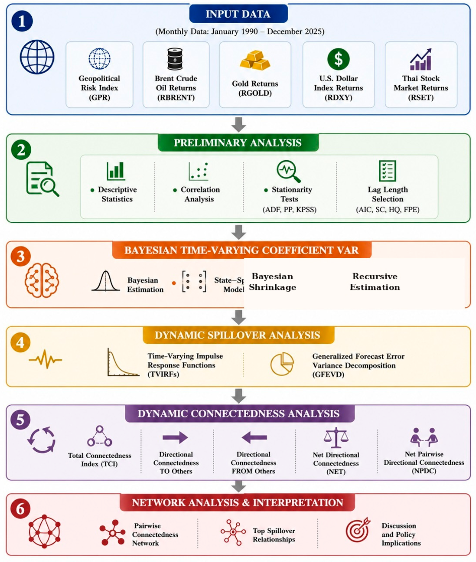
Overall, the proposed framework integrates Bayesian time-varying estimation, TVIRFs, GFEVD, dynamic connectedness measures, and network analysis to provide a comprehensive assessment of the evolving transmission of geopolitical risk across commodity, foreign exchange, and equity markets. The overall research framework is presented in Figure 1.

3.2. Bayesian Time-Varying Coefficient Vector Autoregressive (TVC-VAR) Model

To capture evolving cross-market relationships among geopolitical risk, Brent crude oil, gold, the U.S. dollar, and the Thai stock market, this study employs a Bayesian Time-Varying Coefficient Vector Autoregressive (TVC-VAR) model. The model has one specific role: it estimates coefficients that are allowed to evolve through time rather than imposing a single coefficient matrix over the entire sample. The subsequent TVIRF and connectedness measures are transformations of the same estimated dynamic system, not separate models.

The cross-market terms are included because oil, gold, the U.S. dollar, and Thai equities can be linked through commodity pricing, inflation expectations, international capital flows, and common global information. Their inclusion permits these conditional predictive relationships to be estimated jointly. The model does not identify a structural causal channel for each cross effect; the coefficients should therefore be interpreted as time-varying conditional associations within the multivariate system.

This flexibility is useful when cross-market relationships may change across major geopolitical and financial episodes. The TVC-VAR therefore allows gradual parameter evolution without treating the selected events as exogenously imposed structural breaks (Primiceri, 2005; Koop & Korobilis, 2010; Antonakakis et al., 2020).

The model is used here as a parsimonious dynamic specification for estimating evolving conditional relationships; it is not presented as evidence that any particular event caused a parameter shift.

Let the vector of endogenous variables at time $t$ be

$${\mathit{y}}_t=\left[\begin{array}{c}GP{R}_t\\ RBREN{T}_t\\ RGOL{D}_t\\ RDX{Y}_t\\ RSE{T}_t\end{array}\right]$$

(1)

where $GP{R}_t$ denotes the Geopolitical Risk Index, while $RBREN{T}_t$, $RGOL{D}_t$, $RDX{Y}_t$, and $RSE{T}_t$ denote the monthly log changes in Brent crude oil prices, gold prices, the U.S. Dollar Index, and the SET Index, respectively. The SET Index is the principal broad-market equity index of the Stock Exchange of Thailand and is used as the representative benchmark for the Thai stock market.

The standard VAR($p$) model is specified as

$${\mathit{y}}_t=c+A_1{\mathit{y}}_{t-1}+\cdots +A_p{\mathit{y}}_{t-p}+{\epsilon }_t$$

(2)

where ${\epsilon }_t\sim N\left(0,\mathsf{\Sigma }\right)$. The standard VAR assumes constant coefficient matrices and covariance matrix throughout the sample, an assumption that may be restrictive in the presence of structural changes (Diebold & Yilmaz, 2014).

To capture evolving relationships among the variables, the Bayesian TVC-VAR allows the coefficient matrices to vary over time. In this study, the expression ‘structural change’ is used only in the descriptive sense of change in the estimated coefficient structure; it is not a claim that the model identifies a separate economic structural break or its causal source. The specification permits gradual coefficient drift, while event-specific direct responses are summarized separately through the TVIRFs.

$$y_t=c_t+A_{1,t}{y}_{t-1}+\cdots +A_{p,t}{y}_{t-p}+{\epsilon }_t$$

(3)

${\epsilon }_t\sim N\left(0,{\mathsf{\Sigma }}_t\right)A_{i,t}$ where the coefficient matrices evolve over time. In this study, this evolution is interpreted as time variation in the estimated conditional relationships, not as a separately identified causal structural break.

The TVC-VAR is written in state-space form to allow the coefficient vector to evolve over time. The baseline implementation is coefficient-driven and does not estimate a separate stochastic-volatility process of the full Primiceri (2005) type. Accordingly, the model should not be interpreted as a full TVP-VAR-SV specification.

$${\mathit{y}}_t=Z_t{\mathit{\beta }}_t+{\mathit{\epsilon }}_t$$

(4)

where $Z_t$ contains the intercept and lagged endogenous variables included in the TVC-VAR, ${\beta }_t$ is the vector of time-varying coefficients, and ${\epsilon }_t$~$N\left(0,R_t\right)$ is the disturbance term. No additional exogenous controls are included in $Z_t$.

State equation

The coefficient vector evolves according to a random walk process:

$${\mathit{\beta }}_t={\mathit{\beta }}_{t-1}+{\mathit{\eta }}_t,$$

where

$${\mathit{\eta }}_t\sim N\left(0,Q\right).$$

This specification allows the coefficients to evolve gradually over time and has become the standard Bayesian TVC-VAR formulation (Primiceri, 2005; Nakajima, 2011).

The innovation covariance is allowed to enter the time-varying connectedness calculation through the estimated covariance sequence produced by the implementation, but no separate stochastic-volatility state equation is estimated. This restriction is important during high-volatility episodes because some variance changes may be reflected in the estimated transmission structure. The connectedness results are therefore interpreted as conditional statistical spillovers rather than as a decomposition that separately identifies coefficient drift and stochastic volatility.

The posterior distribution is obtained using Bayes’ theorem:

$$P\left(\theta \mid Y\right)={\displaystyle \frac{P\left(Y\mid \theta \right)P\left(\theta \right)}{P\left(Y\right)}}$$

(5)

where $P\left(Y\mid \theta \right)$ is the likelihood, $P\left(\theta \right)$ is the prior distribution, and $P\left(\theta \mid Y\right)$ is the posterior distribution. Bayesian estimation combines prior and sample information to estimate the time-varying parameters.

Compared with a conventional constant-parameter VAR, the TVC-VAR framework allows the transmission coefficients to evolve over time and is therefore useful for describing changing cross-market relationships. This flexibility does not by itself establish superiority over every alternative dynamic model, and the baseline specification should not be interpreted as a full stochastic-volatility TVP-VAR.

3.3. Time-Varying Impulse Response Function (TVIRF)

Following the estimation of the Bayesian Time-Varying Coefficient Vector Autoregressive (Bayesian TVC-VAR) model, this study employs the Time-Varying Impulse Response Function (TVIRF) to examine how financial markets respond to geopolitical shocks over time. Unlike the conventional impulse response function (IRF), which assumes constant model parameters, the TVIRF allows impulse responses to vary across different periods, thereby capturing structural changes associated with major geopolitical and financial episodes (Primiceri, 2005; Koop & Korobilis, 2010).

The estimated Bayesian TVC-VAR model is expressed as

$$y_t=c_t+{\displaystyle \sum _{i=1}^p}{A}_{i,t}{y}_{t-i}+{\epsilon }_t$$

where the coefficient matrices $A_{i,t}$ evolve over time. Accordingly, the impulse response at forecast horizon $h$ is defined as

$$IR{F}_t\left(h\right)={\displaystyle \frac{\partial y_{t+h}}{\partial {\epsilon }_t}}$$

(6)

Because the coefficients vary over time, the impulse responses also change across different market conditions. The TVIRF therefore captures the dynamic effects of a one-standard-deviation shock to geopolitical risk on each financial variable, allowing the transmission mechanism to evolve with changing economic and geopolitical environments (Antonakakis et al., 2020; Gabauer, 2021).

In this study, the TVIRFs are evaluated during five major episodes: the Gulf War (1990), Global Financial Crisis (2008–2009), the Sovereign-debt period (2012), the COVID-19 pandemic (2020), and the Russia–Ukraine conflict (2022). Comparing responses across these episodes provides insight into how the transmission of geopolitical shocks changes under different crisis regimes and forms the basis for the subsequent connectedness analysis.

3.4. Generalized Forecast Error Variance Decomposition (GFEVD)

Following the estimation of the Bayesian TVC-VAR model, the Generalized Forecast Error Variance Decomposition (GFEVD) is employed to quantify the proportion of forecast error variance explained by shocks originating from other variables. Unlike the Cholesky-based variance decomposition, the generalized approach is invariant to variable ordering, making it suitable for measuring spillover effects in multivariate systems (Pesaran & Shin, 1998; Diebold & Yilmaz, 2012).

The GFEVD is defined as

$${\theta }_{ij}^g\left(H\right)={\displaystyle \frac{{\sigma }_{jj}^{-1}{\displaystyle {\sum }_{h=0}^{H-1}}(e_i^{\prime }{A}_h\mathsf{\Sigma }{e}_j{)}^2}{{\displaystyle {\sum }_{h=0}^{H-1}}(\left.e_i^{\prime }{A}_h\mathsf{\Sigma }{A}_h^{\prime }{e}_i\right)}}$$

(7)

where ${\theta }_{ij}^g\left(H\right)$ denotes the contribution of shocks in variable $j$ to the $H$-step-ahead forecast error variance of variable $i$, $A_h$ is the moving-average coefficient matrix, $\mathsf{\Sigma }$ is the covariance matrix of innovations, $e_i$ is a selection vector, and ${\sigma }_{jj}$ is the standard deviation of the innovation for variable $j$.

Because the generalized variance decomposition does not satisfy the adding-up constraint, each row is normalized as

$${\tilde{\theta }}_{ij}^g\left(H\right)={\displaystyle \frac{{\theta }_{ij}^g\left(H\right)}{{\displaystyle {\sum }_{j=1}^N}{\theta }_{ij}^g\left(H\right)}}$$

The normalized GFEVD forms the basis for the Total Connectedness Index (TCI), directional connectedness (TO and FROM), net connectedness (NET), and net pairwise directional connectedness (NPDC).

3.5. Dynamic Connectedness Measures

Based on the normalized GFEVD, the dynamic connectedness analysis follows Diebold and Yilmaz (2012, 2014) and Antonakakis et al. (2020). The reported TCI, TO, FROM, NET, and NPDC measures are calculated for the four financial markets—RBRENT, RGOLD, RDXY, and RSET. GPR is used in the preceding GPR-transmission/TVIRF stage and is not a fifth node in the reported connectedness system.

The Total Connectedness Index measures the overall degree of spillover across all variables in the system. A higher TCI indicates stronger interconnectedness and greater transmission of shocks among financial markets.

$$TCI={\displaystyle \frac{{\sum }_{i\ne j}{\tilde{\theta }}_{ij}^g}{N}}\times 100$$

(8)

where ${\tilde{\theta }}_{ij}^g$ denotes the normalized generalized forecast error variance decomposition and $N$ represents the total number of endogenous variables. The TCI summarizes the proportion of forecast error variance that originates from cross-market spillovers rather than from own-market innovations (Diebold & Yilmaz, 2012).

Directional connectedness TO others measures the contribution of shocks transmitted from variable $i$ to all remaining variables.

$$T{O}_i=\sum _{j\ne i}{\tilde{\theta }}_{ji}^g$$

(9)

A higher value indicates that the variable acts as a stronger transmitter of shocks to other markets.

Directional connectedness FROM others measures the proportion of forecast error variance received by variable $i$ from shocks generated by all remaining variables.

$$FRO{M}_i=\sum _{j\ne i}{\tilde{\theta }}_{ij}^g$$

(10)

Variables with larger FROM values are more vulnerable to external shocks and therefore behave primarily as shock receivers.

Net connectedness is calculated as the difference between outgoing and incoming spillovers.

$$NE{T}_i=T{O}_i-FRO{M}_i$$

(11)

A positive NET value indicates that the variable functions as a net transmitter of shocks, whereas a negative value implies that the variable is a net receiver. Variables with NET values close to zero perform a balanced role by simultaneously transmitting and receiving shocks (Diebold & Yilmaz, 2014).

To examine bilateral spillover relationships, this study employs the Net Pairwise Directional Connectedness (NPDC) measure, defined as

$$NPD{C}_{ij}={\tilde{\theta }}_{ji}^g-{\tilde{\theta }}_{ij}^g$$

(12)

A positive NPDC value indicates that variable $i$ is a net transmitter of shocks to variable $j$, whereas a negative value indicates that variable $i$ is a net receiver. The NPDC measure is used to construct the pairwise connectedness network (Gabauer, 2021).

Together, the connectedness measures provide a comprehensive assessment of the magnitude and direction of spillover transmission within the financial system.

3.6. Data and Variable Construction

The source data span January 1990 to December 2025. After constructing the logarithmic first differences for the four financial series, the balanced estimation sample contains 431 monthly observations from February 1990 to December 2025. The GPR-transmission/TVIRF stage uses GPR, RBRENT, RGOLD, RDXY, and RSET; the connectedness stage uses the four financial-market block (RBRENT, RGOLD, RDXY, and RSET), with variance shares normalized within that four-market system.

The Geopolitical Risk Index (GPR) is from Caldara and Iacoviello (2022). Brent crude oil, gold, and U.S. Dollar Index data are obtained from Investing.com, and the SET Index data were obtained from the SETSMART database of the Stock Exchange of Thailand. For Brent crude oil, RBRENT is defined strictly as the monthly logarithmic price change. The same logarithmic first-difference operator is applied to the gold price, U.S. Dollar Index, and SET Index to construct stationary monthly market-change series. These transformations are reported in decimal units and are not multiplied by 100.

$$R_t=\ln \left({\displaystyle \frac{P_t}{P_{t-1}}}\right)$$

(13)

Before estimating the Bayesian TVC-VAR model, descriptive statistics, correlation analysis, unit root tests, and lag-order selection are conducted. The selected lag structure is then used for the Bayesian TVC-VAR estimation and subsequent connectedness analysis.

Table 1. Description of Variables.

Variable	Description	Transformation	Source	Frequency
GPR	Geopolitical Risk Index	Level	Caldara and Iacoviello (2022)	Monthly
RBRENT	Brent crude oil log price change	Δln(Price)	Investing.com	Monthly
RGOLD	Gold log return	Δln(Price)	Investing.com	Monthly
RDXY	U.S. Dollar Index log return	Δln(Index)	Investing.com	Monthly
RSET	SET Index log return	Δln(Index)	SETSMART	Monthly

Note: Δln(Price) and Δln(Index) denote monthly logarithmic price or index changes in decimal form. In particular, RBRENT is defined as the Brent crude oil log price change. A value of 0.01 represents an approximate 1% monthly change.

summarizes the variables, transformations, and data sources.

4. Results

4.1. Descriptive Statistics

Table 2. The descriptive statistics of GPR, RBRENT, RGOLD, RDXY and RSET.

Statistic	GPR	RBRENT	RGOLD	RDXY	RSET
Mean	103.3794	0.002561	0.005440	0.000127	0.000903
Median	91.4600	0.006225	0.001356	−0.000745	0.005201
Maximum	512.5300	0.379588	0.151872	0.097517	0.284275
Minimum	39.0500	−0.633933	−0.204083	−0.065125	−0.359188
Std. Dev.	50.4131	0.096055	0.043898	0.023089	0.078717
Skewness	3.9223	−0.7079	−0.0795	0.3324	−0.3193
Kurtosis	26.1537	8.8963	4.2286	3.8288	6.0592
Jarque–Bera	10,732.44	660.34	27.56	20.27	175.39
Jarque–Bera p-value	0.0000	0.0000	0.000001	0.000040	0.0000
Observations	431	431	431	431	431

reports the descriptive statistics of the Geopolitical Risk Index (GPR), Brent crude oil log price changes (RBRENT), gold log price changes (RGOLD), the U.S. Dollar Index log changes (RDXY), and the Thai stock-index log changes (RSET) for the balanced estimation period from February 1990 to December 2025.

The results indicate substantial heterogeneity across the variables. The GPR index has a mean of 103.38 and a maximum of 512.53. Among the transformed financial series, RGOLD has the highest average monthly log change (0.54%), followed by RBRENT (0.26%), while RDXY and RSET have smaller sample means.

RBRENT has the largest standard deviation (0.0961), followed by RSET (0.0787). These statistics indicate greater unconditional variability in those series over the sample; by themselves, they do not establish sensitivity to global or geopolitical shocks. RDXY has the smallest standard deviation (0.0231), indicating lower unconditional variability relative to the other transformed financial series.

The distributional characteristics depart from normality. GPR is highly positively skewed and strongly leptokurtic, while RBRENT and RSET display negative skewness. All four transformed financial series exhibit fat tails to varying degrees. These distributional statistics describe the unconditional data distribution and are not, by themselves, evidence of time-varying coefficients.

The Jarque–Bera tests reject normality for all variables (p < 0.01). This non-normality is reported as a feature of the data, not as the reason for selecting the Bayesian TVC-VAR. The TVC-VAR is selected because the research question concerns evolving cross-market relationships and connectedness; Bayesian shrinkage is used to regularize estimation of the time-varying parameter system.

4.2. Correlation Analysis

Table 3. Pearson Correlation Matrix.

Variables	GPR	RBRENT	RGOLD	RDXY	RSET
GPR	1.000	−0.092	0.040	−0.025	0.003
RBRENT	−0.092	1.000	0.159	−0.226	0.124
RGOLD	0.040	0.159	1.000	−0.370	0.143
RDXY	−0.025	−0.226	−0.370	1.000	−0.089
RSET	0.003	0.124	0.143	−0.089	1.000

Note: Values represent Pearson correlation coefficients.

presents the Pearson correlation coefficients among the Geopolitical Risk Index (GPR), Brent crude oil log price changes (RBRENT), gold log price changes (RGOLD), the U.S. Dollar Index log changes (RDXY), and the Thai stock-index log changes (RSET).

GPR has weak full-sample contemporaneous correlations with the four financial series (RBRENT −0.092, RGOLD 0.040, RDXY −0.025, RSET 0.003). These values describe static linear association only; they neither demonstrate time variation nor rule out lagged or time-varying relationships. The TVC-VAR is motivated by the research question about evolving dynamics, not by the size of these static correlations.

4.3. Stationarity Tests

Table 4. Unit-Root Tests for Model Variables and Underlying Log Price/Index Levels.

Variable	ADF	PP	KPSS	Order of Integration
GPR	−8.168 ***	−8.429 ***	0.134	I(0)
RBRENT	−17.247 ***	−16.982 ***	0.073	I(0)
RGOLD	−22.569 ***	−22.568 ***	0.615	I(0), mixed KPSS evidence
RDXY	−19.333 ***	−19.289 ***	0.055	I(0)
RSET	−19.110 ***	−19.063 ***	0.088	I(0)
ln Brent price (level)	−1.652	—	—	I(1)
ln gold price (level)	1.398	—	—	I(1)
ln U.S. Dollar Index (level)	−2.172	—	—	I(1)
ln SET Index (level)	−1.470	—	—	I(1)

Note: *** denotes rejection of the unit-root null hypothesis at the 1% significance level for the ADF and PP tests.

reports stationarity evidence for both the variables used in the TVC-VAR and the underlying log price/index levels. The ADF tests in levels show that the log levels of Brent crude oil, gold, the U.S. Dollar Index, and the SET Index fail to reject a unit root, whereas their logarithmic first differences are stationary under the ADF and PP tests. GPR is stationary in levels. These results support the selected transformations and reduce concern that the financial series were over-differenced.

Note: ADF and PP test the null hypothesis of a unit root; KPSS tests the null hypothesis of stationarity. For the additional level tests, the ADF regression includes an intercept and zero augmentation lags, consistent with the reported ADF specification for the transformed series. Because cumulative log changes recover each log price/index level only up to an additive constant, the ADF statistic is unaffected by the unknown initial scaling constant. Dashes indicate tests not repeated for the supplementary level rows. *** denotes rejection of the unit-root null at the 1% level. The RGOLD transformation retains mixed evidence because ADF/PP reject a unit root while KPSS rejects stationarity at the conventional 5% level.

The ADF and PP tests have a unit-root null, whereas the KPSS test has a stationarity null. ADF and PP reject a unit root for all five model variables. KPSS is consistent with stationarity for GPR, RBRENT, RDXY, and RSET, but the RGOLD statistic (0.615) rejects the KPSS stationarity null at the conventional 5% level. Thus, the tests provide mixed evidence for RGOLD rather than unanimous evidence of stationarity. Given that RGOLD is already expressed as a monthly log price change and that both ADF and PP strongly reject a unit root, it is retained in the model as an I(0) transformed series, with the KPSS conflict explicitly acknowledged.

The level tests provide the formal basis for transforming the four financial-market series. The ADF statistics for log Brent (−1.652), log gold (1.398), log U.S. Dollar Index (−2.172), and log SET Index (−1.470) do not reject the unit-root null at conventional levels. By contrast, the corresponding log changes strongly reject a unit root. GPR, which enters the model in levels, rejects the unit-root null (ADF = −8.168). Accordingly, GPR enters in levels, while the four financial variables enter as logarithmic first differences. Throughout the analysis, the transformed oil variable is termed the Brent crude oil log price change.

Overall, ADF and PP support stationarity of the model variables, while KPSS gives mixed evidence for RGOLD. RGOLD is retained as an I(0) log-difference series, with this qualification stated explicitly.

Given the mixed KPSS evidence for RGOLD, an additional Zivot–Andrews unit-root test allowing for an endogenous structural break was conducted as a robustness check. The unit-root null is strongly rejected under both the intercept-break specification (test statistic = −23.714; 1% critical value = −5.34) and the intercept-and-trend-break specification (test statistic = −23.808; 1% critical value = −5.57). Both specifications identify the same potential break point in August 2011. These results provide additional support for treating RGOLD as an I(0) transformed series despite the conflicting KPSS result.

4.4. Lag Length Selection

Table 5. VAR Lag Order Selection Criteria.

Lag	LogL	LR	FPE	AIC	SC	HQ
0	2645.474	–	4.69 × 10−11	−12.430	−12.392	−12.415
1	2664.918	38.430	4.62 × 10−11	−12.447	−12.256	−12.371
2	2675.679	21.067	4.73 × 10−11	−12.422	−12.079	−12.286
3	2683.171	14.525	4.93 × 10−11	−12.382	−11.886	−12.186
4	2698.494	29.420	4.94 × 10−11	−12.379	−11.730	−12.123
5	2709.105	20.173	5.07 × 10−11	−12.353	−11.553	−12.037
6	2718.398	17.494	5.24 × 10−11	−12.322	−11.368	−11.945

Note: Bold values indicate the lag order selected by each criterion.

reports the lag order selection results based on the Akaike Information Criterion (AIC), Schwarz Criterion (SC), Hannan–Quinn Criterion (HQ), Final Prediction Error (FPE), and the sequential modified likelihood ratio (LR) test.

The selection criteria provide slightly different recommendations. The AIC and FPE identify Lag 1 as the optimal specification, whereas the SC and HQ criteria favor Lag 0, and the LR test suggests Lag 4. Such differences are common because each criterion applies a different penalty for model complexity.

Following the AIC and FPE criteria, this study adopts a first-order lag structure (Lag = 1) for the Bayesian TVC-VAR estimation. A parsimonious specification is appropriate for the available sample size (431 monthly observations) and helps maintain estimation stability while adequately capturing the dynamic interactions among the variables. Accordingly, all subsequent analyses are based on a first-order Bayesian TVC-VAR model.

4.5. Diagnostic Tests for the Selected Lag Structure

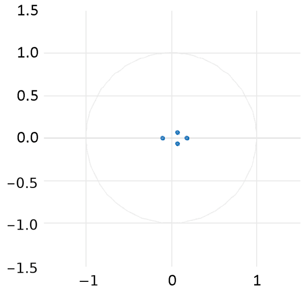
Following the lag-order selection, diagnostic tests were conducted to assess the adequacy and stability of the selected first-order specification. The inverse roots of the AR characteristic polynomial indicate that all roots lie within the unit circle, supporting the stability of the selected lag structure (Appendix B). In addition, the VAR residual serial correlation LM test fails to reject the null hypothesis of no serial correlation at lag 1 (p = 0.1988), indicating that the residuals do not exhibit significant serial dependence (Appendix C). These diagnostic results support the adequacy of the first-order lag specification used in the subsequent Bayesian TVC-VAR estimation.

4.6. Bayesian TVC-VAR Results

4.6.1. Bayesian TVC-VAR Estimation Summary

Table 6. The estimation settings of the Bayesian Time-Varying Coefficient Vector Autoregressive (TVC-VAR) model.

Item	Value
Estimation sample	1990M02–2025M12
Included observations	431
Lag order	1
Estimation engine	Bayesian shrinkage/state-space TVC-VAR
MCMC convergence diagnostics	Not applicable to retained baseline objects
Simulation smoother	Cholesky Factor Algorithm (CFA)
Stability method	Inverse roots of AR characteristic polynomial
Hyperparameters	T0 = 0, τ0 = 5, τ1 = 1, τ2 = 0.01, ν1 = 5, ν2 = 5

summarizes the baseline estimation settings for the Bayesian TVC-VAR using 431 monthly observations and lag order 1.

4.6.2. Time-Varying Coefficient Estimates

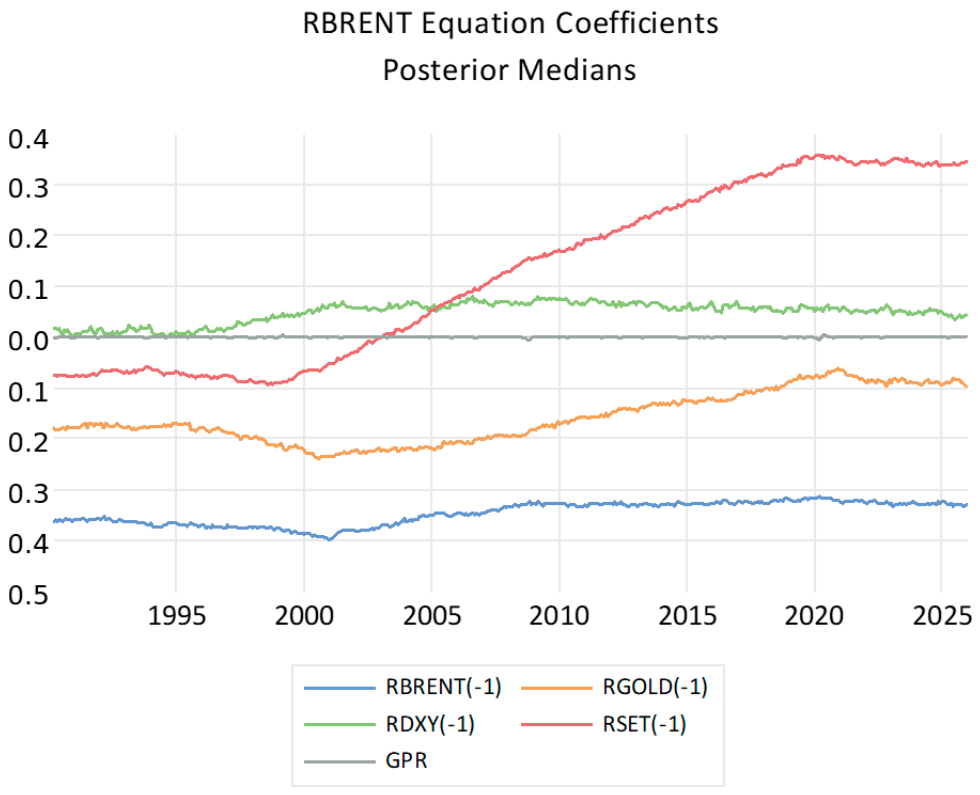
Figure 2 shows the estimated time-varying coefficient paths for the RBRENT equation. The paths are interpreted descriptively; the common-scale graph is not used to date structural breaks, establish significance, or attribute a coefficient movement to a specific event.

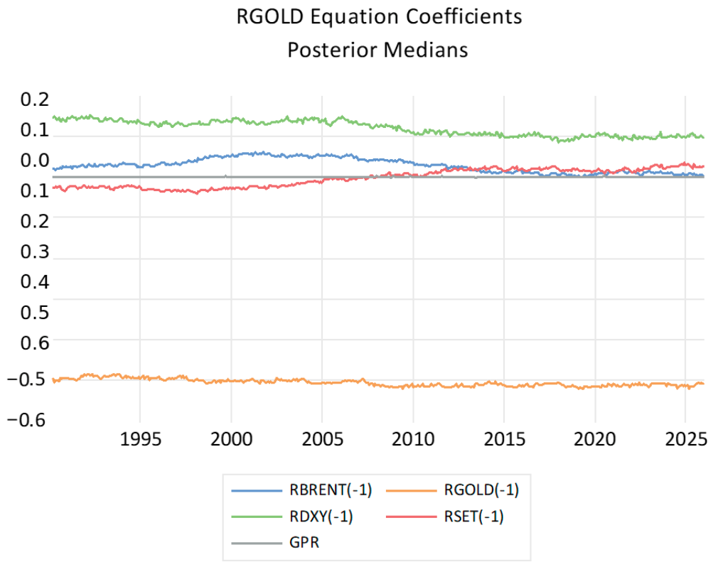
Figure 3 shows the estimated coefficient paths for the RGOLD equation. Because the GPR coefficient is visually small on the common scale, the graph is treated as descriptive parameter-path evidence and is not used to infer a safe-haven role or an event-specific GPR effect.

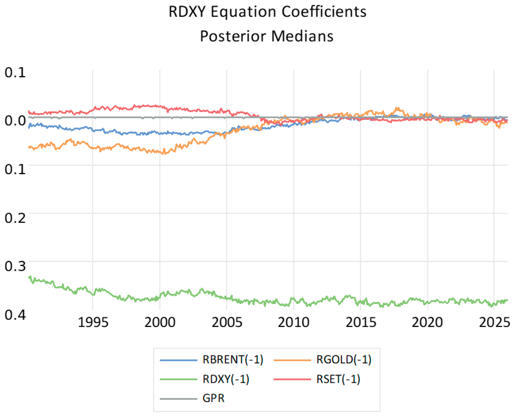
Figure 4 shows the estimated coefficient paths for the RDXY equation. Visual movements are not assigned a causal interpretation; transmitter/receiver roles are assessed from the connectedness measures below.

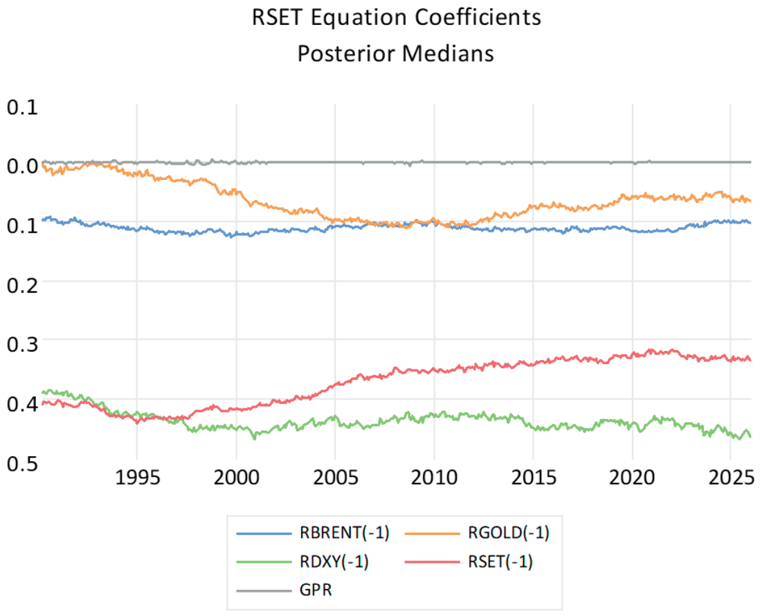
Figure 5 shows the estimated coefficient paths for the RSET equation. The paths indicate time variation in conditional relationships but are not interpreted as event-specific causal effects or formal evidence of significance.

The 1997–1998 Asian Financial Crisis is examined as an additional Thailand-specific robustness episode. The baseline TVC-VAR uses the unchanged full sample and specification, including all observations during the crisis, and the July 1997 state is extracted after re-estimation. The resulting TCI is 13.642%. At this monthly snapshot, RSET is the largest net transmitter (NET = 2.824), while RGOLD is the largest net receiver (NET = −2.818). This evidence is included in the connectedness results reported subsequently. The Asian-crisis check is kept separate from the five pre-selected GPR-shock TVIRF and network episodes because its purpose is to assess a Thailand-centered financial crisis rather than to treat the crisis itself as an exogenously identified GPR shock.

Taken together, Figure 2, Figure 3, Figure 4 and Figure 5 are used only to show that selected conditional relationships evolve over time. They do not identify what drives a shift, whether an event caused it, or whether a plotted movement is statistically significant. Event-specific responses are evaluated with TVIRFs, while system-wide transmission is evaluated with connectedness measures.

At the five pre-selected dates, the coefficient paths show distinct descriptive configurations. In September 1990, RBRENT and RSET rise, RGOLD declines, and RDXY is comparatively stable. In October 2008, October 2020, and February 2022, RBRENT and RGOLD are elevated, RDXY rises, and RSET declines. In August 2012, RGOLD rises and RSET declines, while RBRENT and RDXY show more variable movements. These configurations summarize the plotted coefficient paths only and do not constitute evidence of discrete structural breaks, causal event effects, defensive-asset roles, or statistical significance.

Across the RBRENT, RGOLD, RDXY, and RSET equations, the GPR coefficients are small on the common plotting scale. Formal coefficient-specific posterior bands are not available from the retained baseline output; therefore, Figure 2, Figure 3, Figure 4 and Figure 5 are interpreted as descriptive evidence of time-varying conditional relationships only. The plots are not used to infer coefficient significance, a safe-haven function, or transmitter/receiver status.

4.6.3. Time-Varying Impulse Responses

The time-varying impulse response analysis examines how a one-standard-deviation GPR shock propagates across Brent crude oil, gold, the U.S. Dollar Index, and the Thai stock market over different horizons.

Table 7. Average Generalized Time-Varying Impulse Responses to a GPR Shock.

Variable	h = 1	h = 3	h = 6	h = 12
RBRENT	−0.001149	−0.000178	−0.000095	−0.000046
RGOLD	0.000714	0.000115	0.000040	0.000034
RDXY	0.000911	0.000527	0.000180	0.000034
RSET	0.004456	0.001896	0.000788	0.000180

Note: The table reports the average generalized impulse response of each market to a one-standard-deviation GPR shock over the sample period January 1990–December 2025. The responses are obtained from the Bayesian TVC-VAR framework using time-varying coefficients and covariance matrices. The sample contains 431 monthly observations.

reports the sample-average generalized impulse responses, while

Table 8. Episode-Specific Generalized Time-Varying Impulse Responses to a GPR Shock.

Episode	Date	Response	h = 1	h = 3	h = 6	h = 12
Early geopolitical episode	September 1990	RBRENT	0.024130	0.008974	−0.002071	0.011854
		RGOLD	0.008550	0.000585	0.000633	−0.003009
		RDXY	0.000332	0.002867	−0.000392	−0.008635
		RSET	−0.022106	−0.017624	0.002794	0.002794
Global Financial Crisis	October 2008	RBRENT	−0.002065	−0.000791	−0.000130	0.000041
		RGOLD	0.000125	0.000052	0.000007	−0.000902
		RDXY	−0.000924	−0.000395	−0.000065	−0.007955
		RSET	0.005986	0.002511	0.000413	0.002511
Post-crisis episode	August 2012	RBRENT	−0.001100	−0.000371	−0.000059	−0.001702
		RGOLD	−0.000447	−0.000165	−0.000026	−0.001048
		RDXY	−0.000816	−0.000334	−0.000053	0.003151
		RSET	0.002721	0.001080	0.000172	0.001079
COVID-19 episode	October 2020	RBRENT	0.001905	0.000711	0.000106	−0.000145
		RGOLD	0.000209	0.000068	0.000007	−0.000903
		RDXY	−0.000181	−0.000128	−0.000025	−0.007994
		RSET	0.004174	0.001364	0.000513	0.000078
Russia–Ukraine conflict	February 2022	RBRENT	0.000216	0.000558	0.000209	0.000032
		RGOLD	−0.001289	−0.000448	−0.000172	−0.000026
		RDXY	−0.000125	−0.000124	−0.000048	−0.000007
		RSET	−0.000884	−0.000587	−0.000228	−0.000034

Note: Entries report generalized time-varying impulse responses to a one-standard-deviation GPR shock at the indicated episode dates over horizons of 1, 3, 6, and 12 months.

provides episode-specific responses for five representative geopolitical and financial stress periods.

The average responses in Table 7 are generally largest at short horizons and smaller at longer horizons. RBRENT has a negative sample-average response, while RGOLD, RDXY, and RSET have positive averages. These averages are descriptive and may conceal substantial episode-specific variation.

Table 8 reports the retained episode-specific TVIRF output. Several entries are numerically close or identical after rounding, and some responses are non-monotonic across horizons. These values are therefore not interpreted as monotonic decay patterns. The table is used descriptively to compare the sign and approximate magnitude of responses across episodes, and the discussion avoids drawing conclusions from isolated repeated rounded entries.

A time-varying impulse response need not decay monotonically at every selected horizon; a later-horizon response may therefore differ in sign or magnitude from an intermediate-horizon response. Table 8 is consequently interpreted cautiously, and individual horizon values are treated as descriptive conditional responses rather than precise structural effects.

The February 2022 Russia–Ukraine episode provides an additional recent observation of this time variation. The responses are relatively modest in magnitude and generally decline rapidly across horizons. This does not imply that the conflict had a weak systemic effect, since the connectedness analysis indicates elevated cross-market spillovers during this period. Rather, the result highlights the distinction between the response to a standardized GPR shock and the broader configuration of market connectedness.

Overall, the TVIRF results indicate that the transmission of geopolitical risk is time-varying, heterogeneous across markets, and dependent on the prevailing stress regime. These findings provide a basis for examining the contribution of each market to forecast-error variance through the subsequent GFEVD analysis.

4.7. TVC-VAR Connectedness

The GPR variable serves as the geopolitical shock variable in the TVC-VAR framework, whereas the connectedness analysis focuses on the four financial markets. Building on the time-varying impulse-response results, this section examines the evolution of cross-market connectedness among Brent crude oil, gold, the U.S. Dollar Index, and the Thai stock market. The analysis is based on the generalized forecast error variance decomposition (GFEVD) derived from the Bayesian TVC-VAR model. Following Diebold and Yilmaz (2012, 2014), the GFEVD is used to quantify both the magnitude and direction of shock transmission across markets. The forecast error variance decomposition is evaluated over a 12-month forecast horizon, which provides a medium-term measure of cross-market spillovers while avoiding an excessively short horizon that may capture only transitory responses.

Unlike the TVIRF analysis in the preceding section, which focuses on the response of individual variables to specific shocks, the connectedness analysis considers the system-wide transmission structure. It therefore addresses three complementary questions: (i) how strongly the four markets are interconnected over time, (ii) which markets predominantly transmit or receive shocks, and (iii) which bilateral transmission channels become dominant during major episodes. This distinction prevents the connectedness results from duplicating the event-specific impulse-response analysis.

4.7.1. Total Connectedness

The Total Connectedness Index (TCI) summarizes the proportion of forecast error variance attributable to cross-market spillovers rather than own-market innovations (Diebold & Yilmaz, 2012, 2014). Higher TCI values indicate stronger overall market integration and a greater potential for shocks originating in one market to propagate to the others.

For the baseline specification, the mean TCI is 15.658%, indicating that cross-market spillovers account for approximately one-sixth of forecast-error variation on average. More importantly, connectedness is not constant over time. The selected snapshots yield TCI values of 14.641% in September 1990, 13.642% during the additional Asian Financial Crisis check in July 1997, 26.339% in October 2008, 25.687% in August 2012, 24.472% in October 2020, and 23.537% in February 2022 (

Table 9. Total Connectedness during Selected Episodes.

Episode	Date	TCI (%)	Interpretation
Early-sample episode	September 1990	14.641	Relatively moderate connectedness
Asian Financial Crisis	July 1997	13.642	Thailand-specific robustness episode; RSET is the largest net transmitter
Global Financial Crisis	October 2008	26.339	Highest connectedness among selected episodes
Post-crisis/sovereign-debt period	August 2012	25.687	Persistently elevated connectedness
COVID-19 period	October 2020	24.472	High cross-market connectedness
Russia–Ukraine conflict	February 2022	23.537	High cross-market connectedness

Note: TCI is calculated from the normalized GFEVD using a 12-month forecast horizon. Higher values indicate stronger cross-market spillovers. Selected episodes are used to illustrate changes in the connectedness structure rather than to imply that all major episodes generate identical responses.

).

The highest selected value occurs during the Global Financial Crisis, when TCI reaches 26.339%. Connectedness also remains elevated during the post-crisis/sovereign-debt, COVID-19, and Russia–Ukraine snapshots. The July 1997 Asian-crisis value is lower than these later global-stress observations, but its directional structure is informative for Thailand: RSET is the largest net transmitter and RGOLD the largest net receiver at that date. This result shows that a Thailand-centered crisis can alter market roles even when aggregate connectedness is not at its sample maximum.

Importantly, these results should not be interpreted as evidence that every geopolitical or financial event necessarily produces a sharp increase in aggregate connectedness. Rather, the evidence indicates that the strength of market integration depends on the nature and transmission mechanism of the underlying shock. This interpretation is consistent with the connectedness literature, which emphasizes that spillovers are state-dependent and can change substantially across financial regimes (Diebold & Yilmaz, 2014; Gabauer, 2021).

4.7.2. Net Directional Connectedness

While the TCI measures the overall intensity of connectedness, it does not identify the direction of transmission. The net directional connectedness (NET) therefore provides information on whether each market is predominantly a net transmitter or net receiver of shocks. A positive NET indicates that a market transmits more shocks than it receives, whereas a negative value indicates the opposite (Diebold & Yilmaz, 2014).

Table 10. Average Net Directional Connectedness.

Market	NET	Role
RBRENT	1.116	Net transmitter
RGOLD	0.386	Net transmitter
RDXY	−0.869	Net receiver
RSET	−0.633	Net receiver

Note: NET is defined as directional spillovers transmitted to other markets minus spillovers received from other markets.

shows the average NET positions. RBRENT is the strongest net transmitter (1.116), followed by RGOLD (0.386), while RDXY (−0.869) and RSET (−0.633) are net receivers on average.

The role of Brent crude oil is economically plausible because oil prices affect production costs, inflation expectations, trade balances, and monetary-policy conditions, creating several channels through which oil-market shocks can propagate to financial markets (Hamilton, 2009; Kilian & Park, 2009). Gold also exhibits a positive but substantially smaller net position, indicating that its role is not exclusively that of a shock absorber. Instead, gold can transmit information and portfolio-reallocation effects across markets when investors adjust their positions under changing risk conditions. This interpretation is consistent with evidence that the role of gold varies across market regimes rather than remaining uniformly that of a safe haven (Baur & Smales, 2020).

The negative NET value for the Thai stock market indicates that SET is predominantly exposed to external shocks. This result is particularly relevant for an emerging and highly externally integrated market, where international commodity and financial-market developments can affect domestic asset prices through capital flows, exchange rates, and investor risk appetite (Balcilar et al., 2018).

The U.S. Dollar Index also acts as a net receiver in the baseline specification. This result is important because it cautions against characterizing the U.S. dollar as the dominant transmitter solely on the basis of its international reserve-currency status. Its role in the connectedness system is instead state-dependent, which is examined further through the episode-specific and pairwise results below.

4.7.3. Episode-Specific Changes in Market Roles

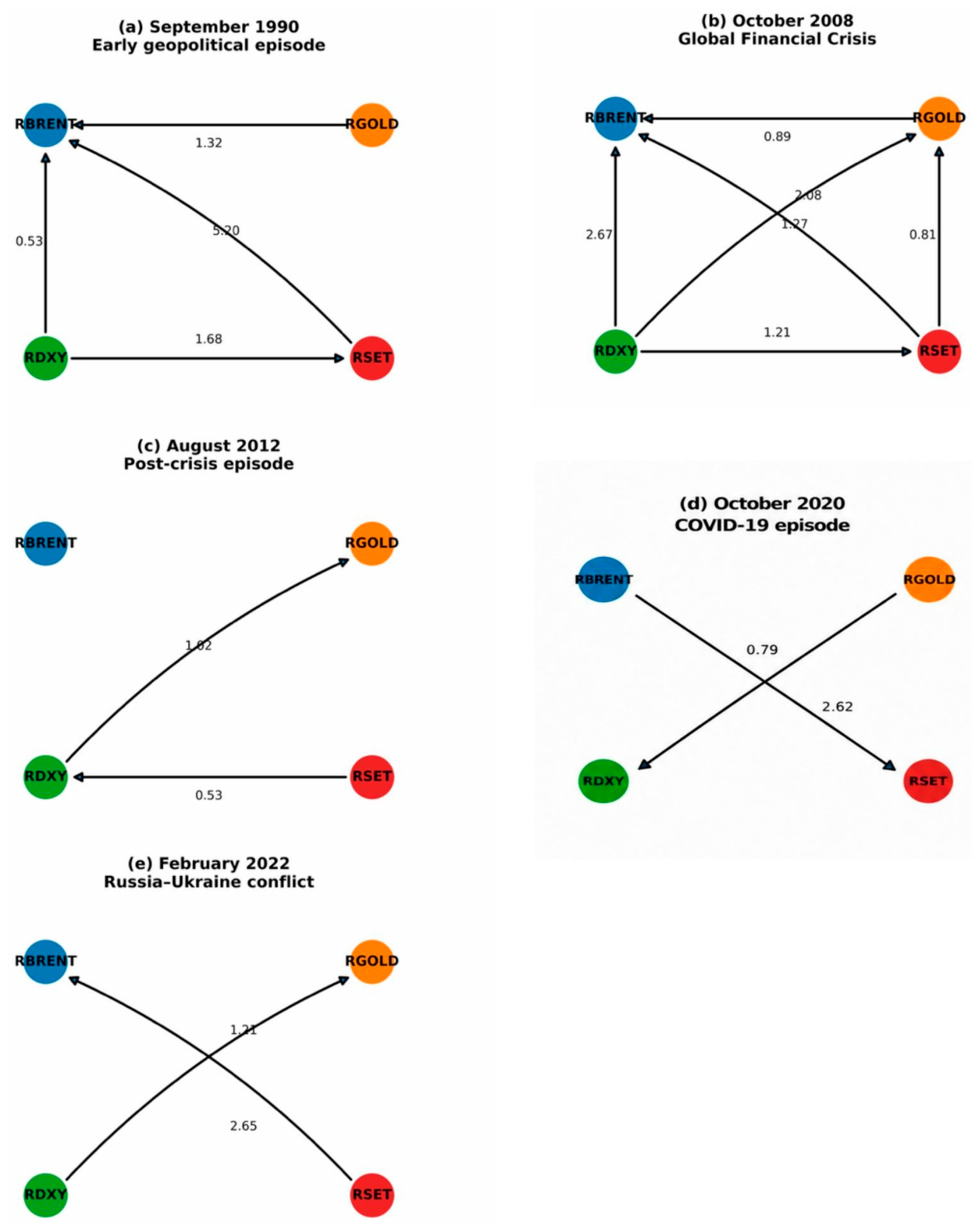
The average NET measures can mask substantial changes in market roles over time.

Table 11. Market Roles and Dominant Pairwise Spillovers across Selected Episodes.

Episode	Date	TCI (%)	Main Transmitter	NET	Main Receiver	NET	Dominant Pairwise Channel	NPDC (%)
Early-sample episode	September 1990	14.641	RBRENT	7.050	RSET	−3.784	RSET → RBRENT	5.203
Global Financial Crisis	October 2008	26.339	RBRENT	4.827	RDXY	−5.955	RDXY → RBRENT	2.672
Post-crisis/sovereign-debt period	August 2012	25.687	RDXY	1.756	RSET	−1.257	RGOLD → RDXY	1.025
COVID-19 period	October 2020	24.472	RSET	2.400	RBRENT	−2.475	RBRENT → RSET	2.621
Russia–Ukraine conflict	February 2022	23.537	RSET	2.390	RBRENT	−2.761	RSET → RBRENT	2.653

Note: NET is an aggregate market-level balance (TO minus FROM across all counterparties), whereas NPDC is a bilateral net balance for a particular pair. Therefore, a market can be a net transmitter in aggregate while receiving from one specific counterparty or be a net receiver in aggregate while transmitting to another specific market. The arrow in the dominant-pairwise column follows the NPDC direction convention used consistently in Appendix A. These directional measures are statistical variance-decomposition relationships and are not interpreted as causal price-setting effects.

therefore reports the dominant transmitter, dominant receiver, and strongest bilateral transmission channel across five representative episodes. The results indicate clear changes in the location and direction of spillover transmission. The dominant transmitter changes across episodes, with RBRENT leading in September 1990 and October 2008, RDXY in August 2012, and RSET during both the COVID-19 and Russia–Ukraine episodes. The dominant bilateral channel also changes across episodes, indicating that the source and direction of transmission are not stable over time.

The episode dates are event-centered monthly snapshots selected to illustrate the estimated network at salient points in time. They are not treated as six-month episode averages or as formal estimates of an entire crisis regime. Because a single monthly state can be noisy, cross-episode differences in Table 11 are interpreted descriptively and are complemented by the uncertainty analysis in Section 4.7.5. A window-averaged episode design remains an important extension for future work.

The Russia–Ukraine episode provides further evidence of this time variation. In February 2022, aggregate connectedness remained relatively high at 23.537%, with RSET becoming the dominant net transmitter (NET = 2.390) and RBRENT the largest net receiver (NET = −2.761). The strongest bilateral channel was RSET → RBRENT, with an NPDC of 2.653%. This represents a reversal from the COVID-19 episode, when the dominant bilateral channel ran from RBRENT to RSET.

Overall, the episode-specific results demonstrate that market roles are state-dependent rather than fixed. The changes in transmitter–receiver positions and bilateral channels provide evidence that geopolitical and financial stress can reconfigure the structure of cross-market spillovers.

4.7.4. Pairwise Connectedness Network

The network analysis provides a complementary view of bilateral shock transmission. While the TCI measures the overall intensity of connectedness and NET identifies the aggregate transmitter–receiver position of each market, the NPDC network shows how individual bilateral channels are organized within the system (Diebold & Yilmaz, 2014; Gabauer, 2021).

4.7.5. Bootstrap Sensitivity Analysis of Connectedness Uncertainty

Appendix D reports a residual-bootstrap sensitivity analysis using 200 replications of the reconstructed TVC-VAR specification. These intervals are bootstrap confidence intervals, not posterior credible intervals. Because the original baseline estimation did not retain posterior draws of the derived TCI, NET, and NPDC measures, the bootstrap exercise is reported as an additional uncertainty check rather than as formal posterior uncertainty around the original baseline point estimates.

For NET, the bootstrap results show that some transmitter-receiver classifications are more stable than others. Brent remains a net transmitter and SET a net receiver at the 90% bootstrap level in the 2008 and 2012 reconstructed episodes, whereas several other market roles have intervals that include zero.

For the 2020 and 2022 episodes, the 90% bootstrap intervals for all four NET measures include zero. The apparent role changes in the baseline point estimates are therefore described as episode-specific descriptive reconfigurations, not as statistically distinguishable regime reversals. The early-sample 1990 bootstrap results are especially wide and should be interpreted with additional caution.

Figure 6 and Appendix A show substantial changes in network topology across the five selected episodes. The September 1990 and October 2008 networks are relatively more interconnected, whereas the August 2012 and October 2020 networks are more concentrated. The February 2022 Russia–Ukraine network exhibits a distinct structure, with the strongest bilateral channel running from RSET to RBRENT and an additional transmission link from RGOLD to RDXY. These differences indicate that similar levels of aggregate connectedness can coexist with substantially different bilateral transmission structures.

This distinction is particularly evident when comparing 2008 and 2012. Although their TCI values are similar (26.339% and 25.687%, respectively), their dominant transmitters and bilateral channels differ. Thus, network topology provides information that cannot be obtained from the TCI alone (Diebold & Yilmaz, 2014; Gabauer, 2021).

4.8. Robustness Analysis

Robustness is assessed by comparing the baseline lag-1 TVC-VAR with a lag-2 specification while holding the connectedness horizon at H = 12. As shown in

Table 12. Robustness of Dynamic Connectedness under Alternative TVC-VAR Specifications.

Specification	Lag	Mean TCI (%)	Max TCI (%)
Baseline TVC-VAR	1	15.658	26.339
TVC-VAR(2)	2	16.192	26.363

Note: Both specifications use the same monthly sample (January 1990–December 2025) and forecast horizon (H = 12); only the lag order changes.

, mean TCI changes from 15.658% to 16.192% and maximum TCI from 26.339% to 26.363%.

The corresponding NET correlations are 0.967 (RBRENT), 0.832 (RGOLD), 0.952 (RDXY), and 0.794 (RSET), indicating broad similarity with some market-specific sensitivity. This check applies only to the derived connectedness measures under the alternative lag order; it does not establish robustness of every coefficient path, prior choice, or forecast horizon.

5. Discussion

The TVIRF results show that responses to geopolitical-risk shocks vary across markets, horizons, and selected episodes. This pattern is consistent with H1 in the descriptive sense of time-varying responses, without treating individual coefficient paths as formal evidence of causal significance.

The connectedness results also vary over time and reach higher levels in several major stress episodes, providing support for H2. At the same time, the bootstrap sensitivity analysis indicates that not every apparent episode-specific change is statistically distinguishable, so the evidence is interpreted as time-varying connectedness rather than as a uniform crisis effect.

Full-sample averages identify RBRENT as the strongest net transmitter, whereas selected monthly episodes show different transmitter-receiver configurations. This evidence is consistent with H3, but the role changes are interpreted cautiously because uncertainty intervals are wide in several episodes.

The use of event-centered monthly snapshots should also be interpreted in light of the model diagnostics. The selected first-order specification satisfies the stability condition based on the inverse roots of the AR characteristic polynomial and shows no evidence of residual serial correlation at lag 1, as reported in Appendix B and Appendix C. These diagnostics reduce concern that the reported monthly network configurations are merely artifacts of an unstable or serially misspecified baseline model. They do not, however, establish that a one-month configuration persists throughout an entire crisis window. Accordingly, the episode-specific results remain descriptive point estimates and are interpreted jointly with the bootstrap uncertainty analysis rather than as window-averaged crisis effects.

The NPDC tables and network graphs reveal asymmetric bilateral channels whose dominant direction differs across selected episodes, supporting H4. Episodes with comparable aggregate connectedness can therefore exhibit different network structures and transmission paths (Diebold & Yilmaz, 2014; Gabauer, 2021).

The February 2022 RSET → RBRENT link illustrates why NPDC directions require economic caution. This arrow should not be interpreted as the Thai stock market setting or causing global Brent prices. Within the generalized variance-decomposition framework, it represents a relative predictive transmission relationship in the estimated system. A plausible interpretation is that Thai equities may adjust rapidly to common geopolitical news, regional risk sentiment, exchange-rate conditions, or portfolio reallocation, with related information subsequently reflected in Brent-return dynamics at the monthly horizon. This is therefore better viewed as a common-information or predictive-transmission channel than as a causal price-setting mechanism, particularly because the 2022 bootstrap intervals indicate substantial uncertainty around episode-specific role classifications.

Taken together, the four hypotheses are supported to different degrees by the reported TVIRF, connectedness, NET, and NPDC evidence. The results are interpreted as conditional statistical transmission within the estimated system, not as structural causality. For an emerging market such as Thailand, the findings are therefore most directly relevant to financial-risk monitoring and macro-financial surveillance.

6. Conclusions, Limitations and Policy Implications

6.1. Conclusions

This study examines the dynamic transmission of geopolitical risk across Brent crude oil, gold, the U.S. Dollar Index, and the Thai stock market using a Bayesian Time-Varying Coefficient Vector Autoregressive (Bayesian TVC-VAR) framework over the period from January 1990 to December 2025. The analysis combines time-varying impulse response functions, generalized forecast error variance decomposition, and dynamic connectedness measures to identify changes in the magnitude, direction, and structure of financial-market spillovers.

The results indicate that estimated geopolitical-risk transmission and financial-market connectedness vary over time and across selected episodes. The Global Financial Crisis has the highest TCI among the event-centered point estimates (26.339%). Because the episode analysis is based on monthly snapshots and several uncertainty intervals include zero, these episode-specific results are interpreted as descriptive evidence of time variation rather than as statistically established regime changes.

The residual-bootstrap exercise is treated as a sensitivity analysis under the reconstructed TVC-VAR specification rather than as a posterior credible interval around the original baseline estimates. It shows substantial uncertainty, especially in the early sample, and indicates that several apparent transmitter-receiver changes are not distinguishable at the 90% bootstrap level. This evidence tempers the role-reversal narrative and supports a more cautious interpretation of episode-specific signs.

The baseline point estimates identify Brent crude oil as the strongest average net transmitter and gold as a smaller net transmitter, while the U.S. Dollar Index and Thai stock market are net receivers on average. Episode-specific point estimates show different configurations, but these changes are not uniformly distinguishable once bootstrap uncertainty is considered. Pairwise arrows, including RSET → RBRENT, are therefore interpreted as generalized-decomposition statistical relationships rather than causal price-setting channels.

The time-varying impulse responses provide additional evidence that the magnitude and persistence of GPR effects differ across episodes and horizons. The Russia–Ukraine episode, in particular, does not generate the largest direct impulse responses across the markets, despite maintaining relatively elevated system-wide connectedness. This distinction highlights that direct responses to a GPR shock and broader market connectedness capture different dimensions of geopolitical transmission.

Overall, the findings are consistent with a time-varying and reconfigurable connectedness structure, subject to the limitations of single-month episode snapshots, the absence of a separately estimated stochastic-volatility state equation, and incomplete posterior uncertainty for derived connectedness measures. The robustness evidence is limited to the alternative-lag comparison and should not be generalized to unverified forecast-horizon specifications.

6.2. Policy Implications

The findings have several implications for financial and economic policy. First, policymakers should strengthen integrated macro-financial surveillance systems that jointly monitor geopolitical risk, international oil prices, exchange-rate conditions, and domestic equity-market developments. The increase in connectedness during periods of global stress suggests that monitoring individual markets separately may fail to identify emerging cross-market transmission risks.

Second, the prominent role of Brent crude oil as the average net transmitter suggests that energy security and diversification should remain important components of Thailand’s risk-management strategy. Diversifying energy sources, improving energy efficiency, and promoting renewable energy can reduce the domestic economy’s exposure to externally generated oil-price shocks.

Third, the changing roles of the U.S. Dollar Index and the Thai stock market across episodes suggest that policymakers should adopt state-dependent rather than fixed crisis-management strategies. Exchange-rate monitoring, foreign-exchange liquidity management, and macro-financial stress testing should be strengthened when international spillovers intensify.

Finally, because the Thai stock market is a net receiver on average but becomes a net transmitter during selected episodes, financial regulators should avoid treating market vulnerability as constant. Dynamic stress testing and scenario analysis based on alternative geopolitical and financial regimes would provide a more appropriate basis for assessing systemic risk and identifying potential transmission channels before they intensify.

The reversal in bilateral transmission observed during the Russia–Ukraine episode further suggests that Thailand’s risk-monitoring framework should incorporate regime-specific stress scenarios rather than rely on fixed assumptions about the direction of external shocks.

6.3. Limitations and Future Research

This study has several limitations. First, the analysis focuses on four financial markets—Brent crude oil, gold, the U.S. Dollar Index, and the Thai stock market. Other sources of uncertainty, including interest rates, economic policy uncertainty, financial stress, climate risk, and cryptocurrency markets, may also influence the transmission mechanism.

The study uses the built-in Bayesian shrinkage-prior setting of the ConnectednessApproach R package (version 1.0.4) and does not report a separate prior-sensitivity analysis for the coefficient paths. Future work should vary the package’s shrinkage settings and compare the resulting parameter trajectories to quantify how strongly individual movements depend on prior regularization.

The model is designed to estimate time-varying relationships and connectedness retrospectively within the sample; it does not forecast the timing of future parameter shifts. For contemporary policy use, the results therefore support monitoring and scenario analysis rather than point prediction of the next regime change. A further extension would evaluate whether observed state variables can predict changes in the estimated coefficients or connectedness measures.

Second, the analysis uses monthly observations, which may not capture very short-lived spillovers occurring at daily or intraday frequencies. Future research could employ higher-frequency data to identify more immediate market responses to geopolitical risk shocks.

Third, the study does not estimate a separate stochastic-volatility state equation and does not provide a full benchmark comparison with constant-parameter VAR and rolling-window connectedness models. The TVC-VAR should therefore be viewed as the selected dynamic specification rather than as an empirically proven superior model. Future work should compare TCI paths and forecasting performance across these alternatives.

Fourth, the event analysis uses selected monthly snapshots rather than six-month episode averages. These snapshots are useful for illustrating local network configurations but may be noisy; future research should report window averages and within-window dispersion around each event.

Fifth, the study does not estimate hedge ratios, optimal portfolio weights, or hedging effectiveness. Consequently, the connectedness results should not be interpreted as direct evidence of portfolio diversification or safe-haven performance. Practical implications are restricted to risk monitoring and the identification of statistical transmission channels.

Finally, future studies could extend the analysis to other emerging markets and conduct comparative cross-country analyses to determine whether the transmission architecture identified for Thailand is common across emerging economies or reflects country-specific characteristics.

References

1. Antonakakis, N., Chatziantoniou, I., & Gabauer, D. (2020). Refined measures of dynamic connectedness based on time-varying parameter vector autoregressions. Journal of Risk and Financial Management, 13(4), 84. [Google Scholar] [CrossRef] [Scilit]
2. Balcilar, M., Bonato, M., Demirer, R., & Gupta, R. (2018). Geopolitical risks and stock market dynamics of the BRICS. Economic Systems, 42(2), 295–306. [Google Scholar] [CrossRef] [Scilit]
3. Baur, D. G., & Lucey, B. M. (2010). Is gold a hedge or a safe haven? An analysis of stocks, bonds and gold. Financial Review, 45(2), 217–229. [Google Scholar] [CrossRef] [Scilit]
4. Baur, D. G., & Smales, L. A. (2020). Hedging geopolitical risk with precious metals. Journal of Banking & Finance, 117, 105823. [Google Scholar] [CrossRef] [Scilit]
5. Bouzguenda, M., & Jarboui, A. (2025). Unravelling interconnectedness and dynamic behaviour in financial networks: Insights from asset analysis. Global Business Review. Advance online publication. [Google Scholar] [CrossRef] [Scilit]
6. Caldara, D., & Iacoviello, M. (2022). Measuring geopolitical risk. American Economic Review, 112(4), 1194–1225. [Google Scholar] [CrossRef] [Scilit]
7. Chen, X., Yao, Y., Wang, L., & Huang, S. (2024). How EPU, VIX, and GPR interact with the dynamic connectedness among commodity and financial markets: Evidence from wavelet analysis. The North American Journal of Economics and Finance, 74, 102217. [Google Scholar] [CrossRef] [Scilit]
8. Diebold, F. X., & Yilmaz, K. (2012). Better to give than to receive: Predictive directional measurement of volatility spillovers. International Journal of Forecasting, 28(1), 57–66. [Google Scholar] [CrossRef] [Scilit]
9. Diebold, F. X., & Yilmaz, K. (2014). On the network topology of variance decompositions: Measuring the connectedness of financial firms. Journal of Econometrics, 182(1), 119–134. [Google Scholar] [CrossRef] [Scilit]
10. Gabauer, D. (2021). Dynamic measures of asymmetric & pairwise connectedness within an optimal currency area: Evidence from the ERM I system. Journal of Multinational Financial Management, 60, 100680. [Google Scholar] [CrossRef] [Scilit]
11. Hamilton, J. D. (2009). Causes and consequences of the oil shock of 2007–2008. Brookings Papers on Economic Activity, 40(1), 215–261. [Google Scholar] [CrossRef] [Scilit]
12. Kilian, L., & Park, C. (2009). The impact of oil price shocks on the U.S. stock market. International Economic Review, 50(4), 1267–1287. [Google Scholar] [CrossRef] [Scilit]
13. Koop, G., & Korobilis, D. (2010). Bayesian multivariate time series methods for empirical macroeconomics. Foundations and Trends in Econometrics, 3(4), 267–358. [Google Scholar] [CrossRef] [Scilit]
14. Nakajima, J. (2011). Time-varying parameter VAR model with stochastic volatility: An overview of methodology and empirical applications. Monetary and Economic Studies, 29, 107–142. [Google Scholar]
15. Pesaran, H. H., & Shin, Y. (1998). Generalized impulse response analysis in linear multivariate models. Economics Letters, 58(1), 17–29. [Google Scholar] [CrossRef] [Scilit]
16. Primiceri, G. E. (2005). Time-varying structural vector autoregressions and monetary policy. Review of Economic Studies, 72(3), 821–852. [Google Scholar] [CrossRef] [Scilit]
17. Reboredo, J. C. (2012). Modelling oil price and exchange rate co-movements. Journal of Policy Modeling, 34(3), 419–440. [Google Scholar] [CrossRef] [Scilit]
18. Sari, L. K., Bachtiar, M., Achsani, N. A., & Lestari, R. (2026). Dynamic interlinkages between energy, food and metal prices under the geopolitical tension. Resources, 15(5), 61. [Google Scholar] [CrossRef] [Scilit]
19. Yang, H., An, S., Dong, Z., & Dong, X. (2025). The evolution of the linkage among geopolitical risk, the US dollar index, crude oil prices, and gold prices at multiple scales: A wavelet transform-based dynamic transfer entropy network method. Entropy, 27(11), 1177. [Google Scholar] [CrossRef] [Scilit] [PubMed]
Figure 1. Research Framework of the Study. Note: The empirical analysis begins with monthly data collection, followed by preliminary statistical analysis. The Bayesian TVC-VAR model is estimated to obtain Time-Varying Impulse Response Functions (TVIRFs) and Generalized Forecast Error Variance Decomposition (GFEVD). These estimates are used to construct the Total Connectedness Index (TCI), directional connectedness (TO and FROM), Net Directional Connectedness (NET), and Net Pairwise Directional Connectedness (NPDC). Finally, network analysis summarizes the spillover transmission mechanism and supports the empirical discussion and policy implications.
Jrfm 19 00731 g001
Figure 2. Estimated Time-Varying Coefficients for the RBRENT Equation.
Jrfm 19 00731 g002
Figure 3. Estimated Time-Varying Coefficients for the RGOLD Equation.
Jrfm 19 00731 g003
Figure 4. Estimated Time-Varying Coefficients for the RDXY Equation.
Jrfm 19 00731 g004
Figure 5. Estimated Time-Varying Coefficients for the RSET Equation.
Jrfm 19 00731 g005
Figure 6. Net Pairwise Directional Connectedness Networks.
Jrfm 19 00731 g006