

Article

Benchmark-Sensitive Cryptocurrency Diversification: Evidence from Thai REIT Portfolios

by
Chaiyathad Phutthadet
,
Ausawatap Akartwipart
* and
Chainarong Kaewmuangmoon
Department of Finance and Investment, School of Business and Communication Arts, University of Phayao, Phayao 56000, Thailand
*
Author to whom correspondence should be addressed.
J. Risk Financ. Manag. 2026, 19(9), 682; https://doi.org/10.3390/jrfm19090682
Submission received: 6 August 2026 / Revised: 26 August 2026 / Accepted: 31 August 2026 / Published: 4 September 2026
(This article belongs to the Special Issue Financial Funds, Risk and Investment Strategies)

Abstract

Low correlation alone does not establish an implementable diversification benefit. This study tests whether Bitcoin and Ethereum improved a fixed, retrospectively selected sample of 13 Thai REITs—not a point-in-time investable universe—for a Thai baht-based investor, using dependence-aware bootstrap inference (Bonferroni, Benjamini–Hochberg, and Romano–Wolf correction) across 1562 matched daily observations (16 January 2020–30 June 2026); modelled costs cover quarterly top-level reallocations only, not daily REIT-basket weight maintenance. The most robust finding is a cost, not a benefit: daily 95% conditional value-at-risk deteriorates significantly and consistently across all three correction methods for five of eight crypto-inclusive portfolios. By contrast, the seemingly compelling point-estimate pattern—all eight portfolios show higher Sharpe ratios and smaller maximum drawdowns—does not survive the same scrutiny: none of the eight ΔSharpe improvements is significant under Bonferroni or Benjamini–Hochberg, only the rolling strategy (P9) is significant under Romano–Wolf, and all unadjusted evidence disappears under sample-window sensitivity checks. Annual inclusion margins were driven largely by cryptocurrency performance, while counterfactual re-centering descriptively illustrated declining ΔSharpe as benchmark strength increased; none of the underlying comparisons survived multiplicity adjustment. The findings illustrate how seemingly robust point-estimate gains can fail to survive multiplicity-corrected inference, while a downside-risk cost remains statistically significant across all three multiplicity procedures in the principal specification—a cautionary result for practitioners and future diversification studies alike.

1. Introduction

An investor holding Thai real estate investment trusts (REITs) between 2019 and 2026 had a difficult period. REITs are structurally exposed to interest rates through discount-rate and leverage channels (Allen et al., 2000; Giliberto & Shulman, 2017), and the Bank of Thailand’s policy rate moved through accommodative, tightening, and easing phases over these years: near-zero through the pandemic, a tightening sequence beginning August 2022, and an easing sequence from October 2024 that was still ongoing at the sample’s end. Over much of this period a THB-based REIT portfolio did not reward its holders.
Cryptocurrencies were meanwhile promoted as portfolio diversifiers, largely on the strength of their low correlation with traditional assets (Brière et al., 2015; Bouri et al., 2017). For an investor in the position described above, the question is concrete: would adding Bitcoin or Ethereum to a Thai REIT portfolio have improved outcomes in a way that could actually have been captured?
Answering that question requires more care than the correlation figure alone suggests. Four choices determine whether a measured diversification gain corresponds to anything an investor could have realised. Returns must include distributions, which for REITs are a substantial share of total return. Foreign-currency assets must be expressed in the investor’s own currency, since a THB-based holder bears the exchange-rate movement. Portfolio weights must be formed from information available at the time of allocation rather than from the full sample. And inference must accommodate the non-normality and serial dependence that daily financial returns exhibit. None of these is novel; each is a condition for the answer to mean what it appears to mean.
This paper evaluates crypto–REIT diversification for a THB-based investor under all four conditions simultaneously, asking not only whether a point-estimate benefit emerges but whether it survives dependence-aware, multiplicity-corrected inference, and at what cost in downside risk. The REIT universe examined is a fixed, retrospectively selected sample of 13 constituents drawn from a candidate list current as of the end of 2025 (Section 3.1), not a point-in-time investable universe reconstructed from historical listing records; this distinction, and its implications for how the results should be read, are addressed directly in Section 5.4. We take our framing from portfolio theory rather than from the empirical literature: the classical condition under which adding an asset raises a portfolio’s Sharpe ratio depends on the portfolio’s own Sharpe ratio, which implies that a measured diversification benefit is partly a statement about the benchmark. Section 2 develops this into four testable hypotheses before any data are examined—three concerning the Sharpe ratio marginal condition and a fourth concerning downside-risk cost—and, as the results below show, the point-estimate Sharpe ratio pattern the first three target does not survive the same inferential standard that confirms the fourth, a distinction central to how this paper’s findings should be read.
Our closest antecedent is Odusami and Akinsomi (2024), who evaluate dynamic dependence and hedging benefits between Bitcoin, Bitcoin futures, and global and regional REIT indices, finding results that vary by region. We differ in several respects: we examine a single emerging market rather than an index aggregate; we evaluate Bitcoin and Ethereum separately, whereas Odusami and Akinsomi focus primarily on Bitcoin and Bitcoin-futures hedging; allocations are constrained, estimated on trailing data, and costed; and variation is examined descriptively across monetary-policy phases. To our knowledge, published evidence focusing specifically on cryptocurrency diversification in Thai REIT portfolios remains limited, and Asian REIT dynamics are known to differ from developed-market counterparts (Pham, 2012).

2. Literature Review and Theoretical Framework

2.1. Cryptocurrency as a Diversifier, Hedge, and Safe Haven

Three distinct properties are often conflated in this literature: a diversifier has, on average, low correlation with a reference portfolio; a hedge has, on average, non-positive correlation; and a safe haven protects specifically during extreme downturns, a property that need not hold on average. Brière et al. (2015) provided one of the earliest portfolio-based demonstrations of Bitcoin’s low correlation with traditional assets, and Bouri et al. (2017) found Bitcoin is generally a poor hedge but a diversifier through low correlation, with safe-haven behaviour confined to extreme weekly declines in Asian stock markets.
Later work shows all three properties are conditional on market state: hedge capacity weakens in downtrend markets (Bossman et al., 2024), cryptocurrencies become positively correlated with equities during turmoil despite normal-condition disconnection, with safe-haven evidence confined to Dogecoin rather than Bitcoin or Ethereum (Jana & Sahu, 2024), and Bitcoin functions as an inflation hedge without functioning as a safe haven (Choi & Shin, 2022). Ali et al. (2025) find hedging and safe-haven relationships differ in strength between Bitcoin and Ethereum, motivating our separate evaluation of the two throughout this study.
Cryptocurrency is not the only asset class with low correlation to REITs; several sectors, including consumer staples and food-and-beverage equities, share this property empirically. The theoretical case for examining cryptocurrency specifically rests on properties distinct from correlation alone: Bitcoin and Ethereum generate no contractual cash flows tied to real economic activity, unlike equities in any sector, so their pricing is not mechanically anchored to the business cycle that also drives REIT rental income and, through it, the discount-rate and leverage channels of Section 2.2; Bitcoin’s supply follows a fixed, algorithmically determined issuance schedule rather than a supply response to price, a structural feature no equity sector shares; and cryptocurrency allocation is an active policy question for Thai institutional investors specifically, following regulatory developments permitting limited digital-asset exposure, which motivates evaluating it directly rather than as an illustrative example of a low-correlation asset class in general. These properties bear on why the correlation is low, not on whether it is low, and low correlation alone is not the basis for the marginal condition developed in Section 2.4, which depends on the candidate asset’s own Sharpe ratio and the benchmark’s as well.

2.2. REIT Performance, Interest Rates, and Emerging Markets

REITs are structurally exposed to interest rates through two channels: the discount-rate channel, since REIT valuations are commonly modelled as the present value of a distribution stream so a higher discount rate mechanically lowers valuation (Anderson et al., 2022), and the leverage and refinancing channel, since Thai REITs must distribute at least 90% of adjusted net profit and face a 35% leverage ceiling, rising to 60% for investment-grade REITs (Securities and Exchange Commission of Thailand, 2026), increasing reliance on external, interest-rate-sensitive financing. Allen et al. (2000) find REIT interest-rate sensitivity varies with fund characteristics such as asset structure and leverage, and Giliberto and Shulman (2017) and Lin et al. (2022) document this sensitivity empirically across markets and property sectors, with sign and magnitude varying across the interest-rate environment rather than remaining fixed.
REIT distributions are not incidental to this exposure: they are a substantial share of total return, and a price-only series understates performance. For Asian REITs specifically, Pham (2012) documents return and volatility dynamics differing from developed-market counterparts, and Newell et al. (2013, 2015) report strong risk-adjusted performance alongside a limited diversification benefit for French and Singaporean REITs respectively—illustrating that standalone performance and diversification benefit are separable properties, a distinction Section 2.4 formalises. Liow et al. (2017) document return and volatility co-movement across Asian securitised real estate markets more broadly.
We use the interest-rate cycle in this study to partition the sample by an observable characteristic of the REIT benchmark’s environment—not as a causal treatment whose effect on diversification benefit is being estimated. Section 2.4 explains why this distinction matters for how the resulting evidence should be read.

2.3. Implementable Cryptocurrency Portfolio Evidence

Three distinct claims are easily conflated in this literature and are distinguished explicitly throughout this study. Statistical diversification refers only to low correlation between a candidate asset and a reference portfolio (Section 2.1); it is a property of the joint return distribution and requires no portfolio construction at all. Risk-adjusted performance improvement refers to a higher Sharpe, Sortino, or similar ratio for a blended portfolio relative to a benchmark, evaluated at a specific finite weight; Proposition 1 (Section 2.4) shows this depends on statistical diversification but is not implied by it alone. Implementable economic value additionally requires that the improvement survive the frictions this section reviews—currency conversion, transaction costs, estimation error, and out-of-sample portfolio formation—and, in this study, dependence-aware statistical inference with multiple-comparison correction (Section 3.8). A finding at one level does not establish the next: this study documents statistical diversification (Section 4.1) and point-estimate risk-adjusted improvement (Section 4.2), and then shows why neither is sufficient for implementable economic value once inference and multiplicity are addressed (Section 4.3).
A separate strand of the literature asks whether a measured correlation or return benefit corresponds to something an investor could actually have captured, and four issues recur. Currency: Combining USD-denominated Bitcoin and Ethereum data directly with local-currency assets produces a mixed-currency comparison corresponding to no investor’s actual experience, since unhedged currency exposure is known to affect portfolio efficiency and emerging-market diversification conclusions materially (Solnik, 1974; Kaplanis & Schaefer, 1991; Brana & Prat, 2010; Ngo, 2017). Rebalancing and costs: Portfolios evaluated as costlessly rebalanced flatter any strategy relative to one whose frictions are modelled. Estimation error: Mean-variance optimisation amplifies rather than averages out parameter uncertainty (Michaud, 1989), particularly acutely so for cryptocurrency’s short, volatile history. Rolling or out-of-sample formation: Full-sample weights use information unavailable at the time of allocation.
Bakry et al. (2021) evaluate Bitcoin under several portfolio frameworks, and Han et al. (2024) document statistically significant out-of-sample diversification benefits that are robust to alternative benchmarks and rolling-window estimation, though the magnitude depends on the allocation approach and investor risk preference—a form of the benchmark- and specification-dependence this study investigates directly. Cryptocurrency return distributions may also depart from normality, motivating entropy-based alternatives to mean-variance optimisation (Gaied Chortane & Naoui, 2025); this concern, together with potential serial dependence in daily returns, motivates our use of a moving-block bootstrap (Künsch, 1989) rather than asymptotic inference (Section 3.8).
Research gap. Three gaps in this literature motivate the present study. First, the crypto-diversifier literature (Section 2.1) and the REIT interest-rate-sensitivity literature (Section 2.2) have developed largely independently; Odusami and Akinsomi (2024) is the study closest to combining them, but they evaluate Bitcoin and Bitcoin-futures hedging against REIT indices rather than an implementable, cost-inclusive emerging-market portfolio. Second, the implementability literature (Section 2.3) documents that currency alignment, transaction costs, and out-of-sample estimation each materially affect measured diversification benefits, but no study reviewed here applies all four conditions jointly to a Thai REIT–cryptocurrency pairing specifically. Third, and most centrally, none of the studies above formalises how a measured diversification benefit depends on the benchmark’s own risk-adjusted performance, nor examines this dependence by holding the candidate asset fixed and varying benchmark strength; Section 2.4 develops this as a formal proposition and Section 4.5 examines it directly through an algebraic sensitivity exercise rather than a formal empirical test, which is this study’s principal theoretical and empirical contribution.

2.4. Benchmark Dependence in the Sharpe Ratio Framework

For a portfolio holding a weight of (1 − w) in a REIT benchmark and w in a candidate cryptocurrency, the exact Sharpe ratio at any weight w is
S R ( w ) = ( 1 w ) μ R e + w μ C e ( 1 w ) 2 σ R 2 + w 2 σ C 2 + 2 w ( 1 w ) ρ R C σ R σ C ,
where μ R e and μ C e are the REIT’s and the cryptocurrency’s expected excess returns, σ R and σ C are their volatilities, and ρ R C is their correlation. Differentiating SR(w) with respect to w and evaluating at w = 0 isolates the direction in which an infinitesimal allocation moves the portfolio’s Sharpe ratio; this yields the following proposition.
Proposition 1. (Marginal-inclusion condition).
A marginal allocation to the candidate asset C raises the portfolio’s Sharpe ratio above the benchmark’s Sharpe ratio if and only if
S R C > ρ R C × S R R .
Proof (Sketch).
Differentiate SR(w) with respect to w and evaluate at w = 0. The derivative of the numerator is ( μ C e μ R e ), and the derivative of the denominator, using the chain rule on the square root, reduces at w = 0 to ρ R C σ C σ R . Combining terms and signing the derivative positive gives μ C e / σ C ρ R C μ R e / σ R > 0, which rearranges to S R C   > ρ R C × S R R as stated. □
Corollary 1 (Connection to spanning).
Proposition 1 corresponds to the zero-alpha marginal condition: the direction in which adding an infinitesimal allocation to the candidate asset moves the frontier is governed by whether its alpha against the benchmark is zero, a condition equivalent, at the margin, to  S R C  =  ρ R C  ×  S R R . Full Huberman and Kandel (1987) spanning additionally imposes the beta-deviation restriction δ = 1 − b = 0, so that the benchmark’s minimum-variance frontier point is also unaffected. The two conditions are therefore related but not equivalent: Proposition 1’s zero-alpha condition is necessary but not sufficient for full spanning. A bootstrap-based spanning diagnostic, reported in Section 4.1, estimates both parameters via two separate pairwise regressions (Bitcoin on REIT; Ethereum on REIT), though a joint hypothesis test proved numerically unstable and is not reported as inferential evidence (Section 4.1 explains why); the marginal condition is evaluated asset-by-asset, and finite-weight, cost-inclusive performance is evaluated directly in Section 4.2 and Section 4.3, so the three exercises answer related but distinct questions.
This condition is exact only in the limit w → 0. It is a statement about the direction of the derivative of SR(w) at the endpoint, and it does not by itself imply that SR(w) exceeds SR(0) at any particular finite weight such as 5%, 10%, or 20%—the weights this study actually examines. Whether the marginal condition’s implication extends to those finite weights is a separate, empirical question, tested directly in Section 4 rather than assumed.
The marginal-inclusion condition depends jointly on the candidate asset’s Sharpe ratio, its correlation with the benchmark, and the benchmark’s own Sharpe ratio; it does not imply improvement at every finite allocation weight. Critically, the direction of the benchmark effect depends on the sign of ρ R C . When ρ R C > 0, a lower S R R lowers the threshold S R C must clear, so a weaker benchmark makes the condition easier to satisfy. When ρ R C ≈ 0, the threshold is close to zero regardless of S R R , and benchmark strength has little bearing on the condition. When ρ R C < 0, the relationship reverses: a lower S R R raises the threshold. A measured diversification benefit is therefore not generically a statement about the benchmark; it is a statement about the benchmark, conditional on the sign and magnitude of its correlation with the candidate asset—the premise this study investigates empirically rather than assumes.

2.5. Conceptual Framework

Figure 1 summarises the framework used to evaluate cryptocurrency diversification benefits in this study. It begins with an investor-aligned return construction—total-return measurement for the REIT benchmark and THB conversion for cryptocurrency returns (Section 3.3)—which feeds into the asset-level conditions of Section 2.4: cryptocurrency Sharpe ratio, REIT Sharpe ratio, and their covariance. These conditions are translated into realised outcomes through finite portfolio weights, periodic rebalancing, and transaction costs (Section 3.5 and Section 3.6), alongside the evaluation context of the sample window and monetary-policy phase (Section 3.1 and Section 3.2). Portfolio performance is then measured using complementary risk-adjusted and downside-risk statistics (Section 3.7), and dependence-aware bootstrap inference with multiple-comparison adjustment (Section 3.8) assesses whether the estimated improvements are robust.
Monetary-policy phases are used only to examine heterogeneity across periods. The counterfactual re-centering exercise likewise provides a sensitivity analysis rather than causal identification.

2.6. Research Hypotheses

Proposition 1 (Section 2.4) shows that the marginal-inclusion condition depends jointly on the candidate asset’s Sharpe ratio, its correlation with the benchmark, and the benchmark’s own Sharpe ratio, and that it applies only to an infinitesimal allocation, not the 5–20% weights examined here. Whether this condition’s implication extends to finite, cost-inclusive allocations in an emerging market with foreign-exchange exposure—and what determines any departure from it—is an empirical question the marginal condition alone cannot answer. These observations motivate four testable hypotheses. Three (H1–H3) are tied directly to Proposition 1’s marginal-inclusion condition; a fourth (H4) tests a complementary downside-risk cost that the marginal condition, framed only in terms of the mean-variance Sharpe ratio, does not itself predict.
H1 (Marginal condition realised at finite weights).
If Proposition 1’s marginal-inclusion condition holds for Bitcoin and Ethereum against the Thai REIT benchmark, finite-weight allocations of 5–20% should raise point-estimate risk-adjusted performance relative to the REIT-only benchmark, net of currency conversion and transaction costs: ΔSharpe > 0 at the point estimate for every allocation examined.
H2 (Statistical robustness of the finite-weight improvement).
The point-estimate improvements in H1 are statistically distinguishable from zero once the correlation among the eight portfolio comparisons—all sharing the same REIT benchmark—is accounted for: ΔSharpe ≠ 0 under dependence-aware bootstrap inference and multiplicity-adjusted correction.
H3 (Benchmark-strength dependence).
Consistent with Proposition 1’s implication that the marginal-inclusion threshold  ρ R C ×  S R R  falls as  S R R  falls when  ρ R C  > 0, the measured diversification benefit varies inversely with the REIT benchmark’s own risk-adjusted performance: ΔSharpe is larger, and more likely to be statistically distinguishable from zero, during evaluation periods and monetary-policy phases in which the benchmark’s own Sharpe ratio is lower.
Proposition 1 implies that the measured inclusion benefit is conditional on benchmark strength; H3 restates this as a testable empirical claim. The phase comparisons, counterfactual benchmark re-centering, and sample-window robustness tests that follow are used to illustrate this sensitivity, not to provide a causal or independently confirmatory test of it: none establishes that benchmark weakness causes the measured benefit, only that the two vary together as Proposition 1 implies they should under positive correlation, and none of the underlying phase-pair or counterfactual comparisons individually survives multiplicity-adjusted correction (Section 4.4 and Section 4.5). H3 is accordingly not statistically supported after multiplicity correction, although the descriptive pattern observed is consistent with Proposition 1’s implication.
H4 (Downside-risk cost at finite weights).
Independently of whether H1–H3 are supported, larger cryptocurrency allocations increase daily tail risk: The 95% conditional value-at-risk is more negative (worse) at the point estimate for larger allocations, and this deterioration is statistically distinguishable from zero under the same dependence-aware, multiple-comparison-corrected inference applied to H2. Unlike H1–H3, H4 does not follow from Proposition 1’s mean-variance marginal condition, which is silent on tail risk; it tests whether a cost external to that framework is nonetheless present and robust.

3. Data and Method

3.1. Sample, Investment Universe, and Data Sources

The raw sample covers 3 January 2019 to 30 June 2026, giving 1814 daily return observations after differencing. Because the rolling strategy (Section 3.5) requires a 252-day trailing window before its first allocation, it is defined only from 16 January 2020 onward. Every portfolio, including the REIT-only benchmark, is evaluated over this common sample of 1562 observations, so that no comparison confounds a strategy with a difference in evaluation period. This also means the evaluation period begins shortly before the March 2020 market disruption and spans the 2020–2021 cryptocurrency cycle—a consequence of the estimation requirement rather than a choice, and one whose implications Section 4.6 examines directly.
The REIT portfolio is treated as a daily rebalanced, equal-weighted index across 13 SET-listed REITs, selected from a recorded candidate universe of 35 of the 36 SET-listed Thai REITs as of 31 December 2025 (Supplementary Material Table S4a); WHABT was absent from the retained candidate-universe record, and the reason for its omission was not documented; turnover and transaction costs required to maintain this daily equal weighting are not modelled (Section 3.6). The 13 constituents were selected through a documented waterfall (Supplementary Material Table S4a). Thirteen candidates were recorded in the original waterfall as exclusions at the listing-date step, on the premise that they lacked sufficient history for this study’s 2019 sample start; of the remaining 22, screening on price-data coverage over the sample window retained the 13 constituents used here. Individual ticker-level identities for the listing-date step were reconstructed after peer review and independently verified against SET factsheets: nine of the 13 were confirmed listed after 2021; two—CPNREIT and DREIT, both listed in December 2017—were found to have been misclassified, since they in fact predate the 2019 sample start, with their true exclusion reason unestablished because their price history was not retained in the underlying panel data; the remaining two (LHRREIT, QHBREIT) could not be independently confirmed either way. This correction and the full verification record are reported in Supplementary Material Table S4a. Identities and coverage-based reasons for the 9 excluded on coverage grounds were recovered from project records and are also reported there. The 13-REIT universe is nonetheless best described as a fixed, data-available sample rather than a fully reproducible draw from the full market population, given the residual gap for the listing-date step. This initial, cross-sectional screen determines fixed universe membership and is distinct from the ongoing, quarterly liquidity screen described in Section 3.4, which determines which of these 13 constituents are included in the equal-weighted average in any given quarter. All 13 listing dates were independently verified against official SET factsheets and confirm that 12 constituents predate the sample start; the thirteenth, SPRIME, lists three weeks into the sample. Verification also identified a backward-fill artefact for SPRIME: 14 pre-listing price observations (3–22 January 2019) were backward-filled from a later price, and the first-trading-day return (23 January) was found populated when it should have been missing, since no valid prior closing price existed—15 affected return rows in total. This was diagnosed and corrected with no detectable effect on any Section 4.3 ΔSharpe result (Supplementary Material Table S4). Prices and ex-dividend records are from SETSMART (Stock Exchange of Thailand, 2026j). Bitcoin prices are identified as the BTC/USD series for the Binance pair and Ethereum prices as the Ethereum index series, both from Investing.com (2026a, 2026b), with the USD/THB spot rate from the same provider (Investing.com, 2026c); the cited pages reflect the instrument configuration identified during source verification, but the exact export settings in effect at the original data-collection date were not independently logged (Section 5.4). Policy-rate dates are from the Bank of Thailand’s (2026) published history, with the tightening and easing transitions confirmed against the corresponding MPC decision announcements (Bank of Thailand, 2022, 2024).
Two data limitations are stated here rather than deferred. The provider for the daily one-year government bond yield used to construct the risk-free rate is ThaiBMA’s Government Bond Yield Curve (Thai Bond Market Association, 2026), retrieved 4 July 2026, with its construction, trimming, and 16:00 Bangkok-time daily cut-off documented in Section 3.3; a perturbation stress test (Section 3.9, Supplementary Material Table S5B) shows the inferential conclusions are unchanged within the tested range for all eight portfolios, not only P4 and P9. The Bitcoin series is exchange-specific while the Ethereum series is a cross-exchange index, so the two are not constructed on an identical basis; the exact closing time and constituent-exchange weighting underlying the Ethereum cross-exchange index were not retained at the original data-collection date and could not be recovered from the provider’s current public documentation, so small differences in closing conventions between the two series cannot be ruled out and are disclosed here rather than resolved.

3.2. Monetary-Policy Phases

Three phases are defined by actual MPC decisions: an accommodative phase from January 2019 to 9 August 2022 (policy rate 0.50–1.75%), a tightening phase from 10 August 2022 to 15 October 2024 (0.75–2.50%), and an easing phase from 16 October 2024 to June 2026 (1.00–2.25%). The transition dates are the dates on which the Committee’s decisions took effect. We use “phase” rather than “regime” throughout to avoid any implication that these boundaries are being advanced as statistically identified breakpoints in the REIT–cryptocurrency relationship; they are used only to partition the sample by an observable characteristic of the benchmark’s environment, consistent with Section 2.4’s framework.
Phases are defined by observable policy decisions rather than estimated with a Markov-switching model, and their validity as statistical regimes is not separately tested; Section 4.5 evaluates benchmark strength directly through an algebraic sensitivity exercise instead.

3.3. Return Construction and Currency Alignment

REIT returns are total returns. On each ex-dividend date the distribution is added to the price change before the return is computed, so the series reflects what a holder received rather than price appreciation alone. Ex-dividend dates that do not coincide with a valid SET trading observation are matched using the same rule stated at the end of this section for all source series—the distribution is applied on the next available trading-date observation, rather than assumed to occur on a non-trading calendar date. Distributions are recorded gross, before any withholding or investor-level tax; Thai REIT distributions to individual investors are typically subject to withholding tax (10% for most retail investors as of the sample period), so an after-tax investor’s realised total return would be systematically lower than the gross figures reported throughout this study, by an amount depending on the investor’s specific tax position, which is not modelled here. For REITs this distinction is material: distributions are a substantial component of realised return, and a price-only series systematically understates performance.
Cryptocurrency returns are converted to Thai baht before any statistic is computed, via
( 1 + R c r y p t o , t T H B ) = ( 1 + R c r y p t o , t U S D ) ( 1 + R t U S D / T H B )
so that a THB-based investor’s return correctly compounds the asset’s local-currency return with the exchange-rate movement (Solnik, 1974), rather than combining USD-denominated crypto returns directly with THB-denominated REIT returns—a mixed-currency comparison corresponding to no actual investor’s experience. Exchange-rate exposure has been shown to be economically material for REITs specifically (Ngo, 2017) and to alter emerging-market diversification conclusions (Brana & Prat, 2010).
The daily risk-free rate is derived from ThaiBMA’s one-year government bond yield curve (Thai Bond Market Association, 2026), obtained by dividing the annualised yield by 252 trading days. The published curve is constructed from average bids quoted by primary dealers, trimmed by 15% from the top and bottom of the quotes when ranked by value, with a daily cut-off time of 16:00 (Bangkok time) for quotation; the one-year point specifically is a bond-equivalent yield converted from the average simple T-bill yield, consistent with the construction used throughout this study. These parameters are published on the same provider page cited above (Remarks 1, 2, and 4) rather than requiring a separate series identifier, since the yield curve is a constructed, interpolated series across tenors rather than a single priced instrument with its own identifier. Simple returns are used throughout for portfolio aggregation, correlation, and every Sharpe ratio and inclusion-margin calculation reported in this study, since a weighted average of log returns does not equal a portfolio’s return; log returns are not used in any of the reported statistics. Portfolio series are compounded into a wealth process from which all performance statistics are derived, ensuring the mean, standard deviation, and correlation entering Section 2.4’s condition are computed on a single, consistent basis. Non-overlapping SET trading dates are matched to the corresponding calendar-date close of each source series, with the most recent available prior close carried forward where no source-series timestamp coincides with a SET trading date.

3.4. Liquidity Screening

Thai REITs trade thinly, and stale prices depress measured volatility and correlation. Each quarter a constituent enters the equal-weighted basket only if its price changed on at least 50% of trading days in the preceding quarter; constituents failing the screen are excluded for that quarter and re-enter when liquidity recovers. The screen uses only trailing information, so it could have been computed in real time. Across the 30 quarters spanning the raw sample (2019 Q1 to 2026 Q2), a mean of 11.83 of the 13 constituents qualify per quarter (91.0%); the screen binds most tightly in 2019 Q2 (9 of 13 qualifying) and excludes no constituent at all in 12 of the 30 quarters (Supplementary Material Table S11).
Daily turnover data were not available, so this criterion is a proxy for tradability rather than a turnover threshold, which would be the preferable measure. The screened and unscreened REIT series correlate at r = 0.99 over the full sample (Supplementary Material Table S4), indicating the screen changes the benchmark construction only marginally; Section 4.6 re-runs the full downstream pipeline on the unscreened series directly and confirms the study’s principal conclusions are unaffected. The first calendar quarter of the sample (2019 Q1) has no trailing quarter against which to apply the screen, so every constituent listed by that point defaults to being eligible; this default does not make an unlisted constituent investable. SPRIME, not yet listed for the first three weeks of the sample (Section 3.1), has a missing (not zero) return on those pre-listing dates, and the daily equal-weighted REIT return is computed as the mean across only the constituents with a non-missing return that day—effectively renormalising weights among the constituents actually available, rather than assigning a zero or imputed return to an unlisted security. None of the 13 selected constituents delisted, merged, or terminated during the sample. This limits constituent attrition within the selected universe but does not, by itself, eliminate potential selection or survivorship bias arising from the construction of the initial universe (Section 3.1).

3.5. Portfolio Construction

The 5%, 10%, and 20% cryptocurrency weights for P2–P8 were pre-specified before any portfolio was evaluated against the data, following common allocation levels used in the institutional cryptocurrency-allocation literature (e.g., Bakry et al., 2021) rather than being selected after inspecting results; no allocation level was added, removed, or adjusted based on its own performance. The eight portfolios in Table 1 (P2–P9) are treated as one family for multiple-comparison purposes throughout this study because all eight are compared against the same REIT-only benchmark (P1) and were specified together as the full set of allocations this study examines; the Bonferroni, Benjamini–Hochberg, and Romano–Wolf corrections reported in Section 3.8 and Section 4.3 are computed over this pre-specified family of eight, not a subset selected after estimation.
P9 maximises the Sharpe ratio ( E [ R p ] R f ) / σ p subject to weights summing to one, no short positions, and combined cryptocurrency weight not exceeding 20%. The cap is imposed because an unconstrained optimiser on these assets produces corner solutions that no diversified mandate would permit: an unconstrained, full-sample optimisation on this dataset places 100% of the portfolio in Bitcoin. The optimisation is carried out over a transformed parameter space in which the constraints hold by construction, using the Nelder–Mead algorithm (Nelder & Mead, 1965) through optim() in R 4.5.2 (R Core Team, 2025).

3.6. Transaction Costs and Investability

All nine portfolios, including the fixed-weight portfolios, rebalance every 63 trading days. Transaction costs are applied to modelled top-level reallocations among the REIT benchmark, Bitcoin, and Ethereum; earlier treatments of fixed-weight portfolios as costlessly rebalanced each day which flattered them relative to any strategy whose top-level costs were modelled, since such costs were then borne only by the rolling strategy. Turnover at each rebalancing date is computed as the sum of absolute weight changes across these top-level assets required to reset to target (for P2–P8) or to the newly re-optimised weights (for P9). This sum includes both the buy and sell legs of the rebalancing trade and is therefore a two-way (gross) turnover measure, not a one-way measure. Cost is charged as a fixed number of basis points per unit of this two-way turnover, deducted from that day’s portfolio return. P1 (100% REIT, no crypto) shows zero modelled turnover under this measure, since its top-level target weight never changes. The REIT benchmark itself is constructed as a daily equal-weighted average across qualifying constituents (Section 3.4), recomputed each trading day; this is equivalent to daily rebalancing to equal weight within the REIT basket. Turnover and transaction costs required to maintain this daily equal weighting are not modelled for any portfolio, including P1, so P1’s zero modelled turnover reflects the absence of top-level reallocation only, not the absence of internal rebalancing activity. Results throughout this study should be read as net of modelled top-level transaction costs among the REIT benchmark, Bitcoin, and Ethereum—not as fully cost-inclusive, and not as evidence that the REIT benchmark itself is free of rebalancing costs in practice.
Because this daily uncosted internal construction is not itself fully investable, Section 4.6 additionally reports the full pipeline rebuilt with the REIT benchmark instead rebalanced quarterly (the same 63-trading-day frequency as P2–P9) and costed identically to the top-level reallocations described above, both with and without the liquidity screen of Section 3.4. This directly tests whether the paper’s conclusions depend on the benchmark’s own construction being treated as costless.
We retain the daily equal-weight construction as the principal analytical benchmark because it holds the REIT reference portfolio constant and isolates the incremental performance associated with adding cryptocurrency; it is not presented as a fully investable strategy. The quarterly rebalanced and costed construction described above is therefore used as an investability robustness specification, under which the principal multiplicity-adjusted conclusions remain unchanged (Section 4.6).
The baseline cost is 25 basis points per unit turnover; Section 3.9 reports results at 0, 10, and 50 basis points as a sensitivity check. The same per-unit cost is applied to REIT and cryptocurrency legs alike, which is a simplifying assumption—actual trading costs for Thai REITs and for Bitcoin or Ethereum need not coincide, and this study does not attempt to estimate asset-specific costs separately.

3.7. Performance and Risk Measures

Performance is measured by the Sharpe (1966) ratio and, given the positive skewness documented for Bitcoin (Ang et al., 2023), the Sortino ratio (Sortino & Price, 1994). Tail risk is summarised by the maximum drawdown, computed from the compounded wealth index, and the daily 95% conditional value-at-risk (Rockafellar & Uryasev, 2000).
Formulas are stated explicitly. Annualised return is compounded, not arithmetic: (∏(1 + rt))(252/N) − 1, where the product runs over all N daily simple returns in the window. Annualised volatility is the daily standard deviation scaled by √252. The Sharpe ratio is the mean daily excess return (return minus the same-day risk-free rate) divided by the standard deviation of the raw daily return series, annualised by √252; the denominator uses the return series’ own volatility, not the volatility of the excess-return series, consistent with Sharpe’s (1966) original definition. The Sortino ratio uses the same daily risk-free series as the Sharpe ratio; its minimum acceptable return is the sample-average daily risk-free rate over the window in question, and downside deviation is the standard deviation of daily returns falling below that threshold, annualised by √252 in the same way as the Sharpe ratio’s denominator. Daily 95% CVaR is computed historically: the fifth percentile of the daily return distribution is located, and CVaR is the mean of all daily returns at or below that percentile, expressed as a signed percentage—a more negative value indicates a more severe average tail loss, and values are not multiplied by −1 at any point in this study, so all reported CVaR and drawdown figures share the same negative-is-worse sign convention used for returns throughout.

3.8. Statistical Inference

The reported quantity for each comparison is ΔSharpe—the portfolio’s Sharpe ratio minus the benchmark’s—with a 95% percentile confidence interval from a moving-block bootstrap (Künsch, 1989) using a block length of 20 trading days and 10,000 iterations; Section 3.9 reports alternative block lengths as a check on this choice. Reporting an effect size with an interval answers the question an investor asks—how much better, and how sure are we—rather than only whether a null can be rejected. Two-sided p-values accompany the intervals; no conclusion here rests on comparing the magnitude of one p-value with another. All bootstrap resampling, multiplicity corrections, and Sharpe-ratio computations were implemented in R version 4.5.2 (R Core Team, 2025).
The random seed is set immediately before each resampling loop, so every reported figure is a function of the comparison itself and not of its position in the computation. Where several allocations are compared against a common benchmark we report the number of comparisons and the corresponding Bonferroni threshold alongside the unadjusted results. Bonferroni is conservative by design, particularly when the underlying comparisons are correlated, as they are here since every portfolio shares the same REIT benchmark. We therefore report two additional multiplicity-adjustment methods alongside Bonferroni—the single method specified in the original study design—added subsequently at reviewers’ request: Benjamini and Hochberg’s (1995) procedure, which controls the false discovery rate rather than the family-wise error rate that Bonferroni and the method below control, and a Romano and Wolf (2005) stepdown bootstrap that tests each statistic against the bootstrap distribution of the maximum statistic among the remaining hypotheses, directly respecting the correlation structure across portfolios rather than assuming independence. Both are reported for every bootstrap family in this study except ΔMaxDD: our attempted Romano–Wolf implementation for this measure produced invalid or unstable adjusted p-values, so we report only Bonferroni and Benjamini–Hochberg for ΔMaxDD (Supplementary Material Table S7). Although six of eight comparisons are significant at the unadjusted 5% level in the principal ΔSharpe results (Section 4.3), none reaches significance under Bonferroni or Benjamini–Hochberg correction; under Romano–Wolf, which respects the correlation among the eight comparisons directly, the rolling strategy (P9) alone does. This single exception is discussed explicitly in Section 4.3 and Section 5.1 rather than either dismissed or treated as overturning the result under Bonferroni and Benjamini–Hochberg; we report all three methods on equal footing throughout, since no methodological basis favours Bonferroni’s FWER control or Benjamini–Hochberg’s FDR control over Romano–Wolf’s correlation-aware alternative for this correlated, eight-comparison family.
Because daily cryptocurrency and REIT returns may violate joint normality and independence, we rely on moving-block bootstrap inference and do not additionally report the Jobson and Korkie (1981) test.
The bootstrap algorithm is stated explicitly. For each portfolio-versus-benchmark comparison, the baseline (P1) and comparison portfolio’s realised daily excess returns—together with the corresponding daily risk-free rate—are resampled using the identical sequence of block-start indices in every replication, so the same calendar days are drawn for both series and the risk-free rate simultaneously, preserving whatever dependence exists between them. Block-start indices are drawn with replacement from 1 to N − 20 + 1 (N the sample length); blocks do not wrap around the end of the sample (non-circular sampling), so no block spans the first and last observations as if they were adjacent. The required number of 20-day blocks is concatenated and the resulting index sequence truncated to exactly N observations, so the final block contributing to a given replication is typically partial rather than full-length; no separate short-block rule is applied beyond this truncation. This procedure is repeated 10,000 times per comparison, with the random seed reset immediately before each comparison’s resampling loop so that results do not depend on the order in which comparisons are computed. The two-sided bootstrap p-value is twice the smaller of the proportion of replications with ΔSharpe at or below zero and the proportion at or above zero, capped at one.
P9 is not re-optimised within each bootstrap replication. The bootstrap resamples P9’s realised daily returns from the single, historically computed rolling-optimisation path (Section 3.5); it does not redraw the underlying REIT, Bitcoin, and Ethereum returns within each trailing 252-day estimation window or re-solve the constrained optimisation on the resampled data. Consequently, P9’s reported confidence interval reflects sampling uncertainty in which trading days are drawn, conditional on the weights actually realised historically, but does not additionally propagate the parameter-estimation uncertainty inherent in re-optimising on resampled inputs—a source of uncertainty likely to widen P9’s interval further were it included. This is a known limitation of applying block bootstrap inference to a strategy whose weights are themselves estimated rather than fixed, noted here explicitly rather than left implicit, and flagged as a direction for future work in Section 5.4. The block length of 20 trading days follows common practice for daily financial return series exhibiting short-range dependence rather than an automatic block-selection procedure fitted to this sample; Section 3.9 and Section 4.6 report block lengths of 5, 10, 40, and 60 days as a direct check on this choice, and the block-length sensitivity documented there should be read together with this disclosure.

3.9. Robustness and Benchmark-Strength Tests

Nine robustness families assess whether the results in Section 4 depend on specification choices made in Section 3.1, Section 3.2, Section 3.3, Section 3.4, Section 3.5, Section 3.6, Section 3.7 and Section 3.8: excluding 2020 entirely from the evaluation window; an equal-length split of the sample into first and second halves (counted as one family); alternative transaction costs of 0, 10, and 50 basis points; alternative bootstrap block lengths of 5, 10, 40, and 60 trading days; a risk-free-rate perturbation of ±25 and ±50 basis points annually, retained as a robustness check on the risk-free level itself (Section 3.1); an investable REIT-benchmark construction, quarterly rebalanced and costed identically to the top-level legs (Section 3.6), tested both with and without the liquidity screen of Section 3.4; a risk-free-rate timing shift of ±1 trading day, addressing the potential mismatch between ThaiBMA’s 16:00 cut-off and REIT/cryptocurrency closing conventions; and an approximate after-tax adjustment for Thailand’s 10% withholding tax on REIT distributions. Results for all nine are reported in Section 4.6 and Supplementary Material Tables S1–S5, S12 and S16.
One check considered during this study’s development was not included. An annual/quarterly correlation between the benchmark’s own Sharpe ratio and each portfolio’s ΔSharpe was found, by Monte Carlo simulation, to arise mechanically from portfolio arithmetic—a portfolio holding 80% of the same asset as its benchmark cannot have a Sharpe ratio independent of the benchmark’s—rather than from an economic relationship, and was replaced by the counterfactual re-centering exercise in Section 4.5, which does not share this confound.

4. Results

4.1. Return Characteristics and Correlations

Over the matched evaluation window (16 January 2020 to 30 June 2026, N = 1562), the REIT-only baseline lost money: an annualised return of −1.46% and a Sharpe ratio of −0.192 (Table 2). This is the benchmark against which every allocation below is measured, and Section 2.4 explains why its weakness matters for what follows.
REIT–BTC correlation over this window is 0.068 and REIT–ETH correlation is 0.094—both small and positive, indicating weak linear co-movement between cryptocurrency and Thai REIT returns during the sample period. Given these small positive correlations, Section 2.4’s marginal condition implies a weaker REIT benchmark lowers the inclusion threshold, though the effect size scales with the correlation itself and is therefore modest here; had either correlation been zero or negative, benchmark strength would have little bearing on the condition, or the relationship would reverse. All three correlations here, and every Sharpe ratio and inclusion margin reported in this study, are computed on simple returns, matching the return convention used for portfolio aggregation (Section 3.3); a log-return version of these correlations was checked and found materially different for BTC–ETH specifically (0.897 on log returns versus 0.844 on simple returns, a difference of 0.053), which is why the simple-return convention is used uniformly throughout rather than mixed with log returns. The BTC–ETH correlation of 0.844 is not small: Bitcoin and Ethereum moved together over this period, so an allocation split between them (P8) diversifies within crypto only modestly and should not be read as materially more diversified than a single-asset crypto allocation of the same total size.
P9’s realised allocation, averaged across its 25 rebalancing dates over the matched window, held 84.8% in REITs, 7.7% in Bitcoin, and 7.4% in Ethereum—combined cryptocurrency exposure was below the 20% cap on average, though the cap was bound at 16 of the 25 rebalancing dates (64%), materially more often than the average weights alone suggest; full weights and cap-binding status at every rebalancing date are reported in Supplementary Material Table S8.
Improvement is not uniform across risk measures, and the two downside measures diverge with statistical support once each is bootstrapped as its own eight-portfolio multiplicity family (Bonferroni, Benjamini–Hochberg, and Romano–Wolf stepdown; Supplementary Material Table S7). Maximum drawdown falls for every crypto-inclusive portfolio at the point estimate, but this is not statistically significant under Bonferroni or Benjamini–Hochberg for any portfolio; Romano–Wolf is not reported for this measure: our attempted implementation produced invalid or unstable adjusted p-values for ΔMaxDD specifically, so only Bonferroni and Benjamini–Hochberg are reported for it (Supplementary Material Table S7). Daily 95% CVaR—a one-day tail-loss measure, and the object of H4—improves only for P2 (−1.68% versus −1.69% for P1) at the point estimate and worsens for every other portfolio, most sharply for P7 (−2.99%) and P9 (−2.68%); unlike drawdown, this deterioration is statistically significant and robust across all three multiplicity methods for five of eight portfolios (P4, P6, P7, P8, P9), supporting H4. The finding is therefore not that crypto allocations reduce downside risk generally: the full-window maximum drawdown improvement is a descriptively consistent but not robustly significant pattern, while the one-day tail-loss deterioration at larger allocations is both descriptively consistent and statistically robust—a trade-off that is asymmetric in its evidentiary strength, not merely in its direction.
A bootstrap-based spanning diagnostic, connected to Corollary 1’s theoretical link, complements this correlation-based description. For each cryptocurrency, a regression of its daily return on the REIT benchmark’s daily return yields a pricing intercept and a beta-deviation term that jointly determine whether the REIT benchmark alone spans the mean-variance frontier relative to REIT-plus-crypto (Huberman & Kandel, 1987); spanning requires both to be zero. Point estimates and 95% bootstrap confidence intervals for both parameters, for both cryptocurrencies, are reported in Supplementary Material Table S13. A formal joint hypothesis test was attempted using the same moving-block bootstrap methodology as the rest of this study, but is not reported as inferential evidence: Bitcoin’s and Ethereum’s beta-deviation parameters are highly correlated in the bootstrap distribution (correlation 0.95, reflecting the two cryptocurrencies’ own 0.844 return correlation, Section 4.1 above), which makes the joint test’s covariance matrix ill-conditioned (Supplementary Material Table S13); this numerical instability, not the underlying economics, is why no test statistic, p-value, or spanning-rejection claim is reported here. The annualised regression intercepts are large (51.5% for Bitcoin, 72.8% for Ethereum) but reflect the full sample’s 2020–2021 bull-run period and should not be read as an expected forward return. Whether these point estimates constitute meaningful evidence against spanning cannot be established with the inference approach attempted here; what can be said directly is that neither cryptocurrency’s point estimates translate into a finite-weight, cost-inclusive Sharpe ratio improvement distinguishable from zero after multiplicity-adjusted correction (Section 4.3), consistent with Proposition 1’s distinction between the marginal condition and finite-weight performance.

4.2. Point-Estimate Performance

Every crypto allocation examined shows a higher point-estimate Sharpe ratio than the REIT-only baseline, at every weight from 5% to 20% and for both Bitcoin and Ethereum individually. Maximum drawdown is also smaller for every crypto-inclusive portfolio than for the baseline, ranging from −28.5% (P9) to −34.6% (P7) against −42.9% for P1. Section 2.4’s inclusion condition depends jointly on the cryptocurrency’s own Sharpe ratio, its correlation with the benchmark, and the benchmark’s Sharpe ratio, and speaks only to an infinitesimal allocation, not to the 5–20% weights examined here. It also assumes fixed weights and no transaction costs, while the implemented portfolios rebalance quarterly, drift between rebalancing dates, and incur costs, so their finite-weight performance must be evaluated directly. That every weight examined here shows a point-estimate improvement is an empirical finding, examined further in Section 4.5.
The pattern in the point estimates alone would read as unambiguous support for cryptocurrency diversification. Section 4.3 examines whether it survives inference.

4.3. Inference for ΔSharpe

Six of eight intervals exclude zero at the unadjusted 5% level (Table 3); the two 20%-weight single-asset allocations (P4, P7) do not, despite having the largest point estimates, because their bootstrap distributions are also the widest. None of the eight comparisons survives Bonferroni or Benjamini–Hochberg correction for testing eight allocations against a common benchmark (smallest unadjusted p = 0.023 against a Bonferroni threshold of 0.00625). Under the Romano–Wolf stepdown, which respects the correlation among the eight comparisons directly rather than assuming independence, P9 alone survives at the 5% level (p = 0.038); no other portfolio does. In summary: no fixed-weight portfolio survives any of the three multiplicity procedures; P9 survives Romano–Wolf but not Bonferroni or Benjamini–Hochberg, so the inference for P9 depends on the chosen error-control criterion. Whether this single result is judged supported therefore depends on which of the three defensible correction methods is applied: Bonferroni and Benjamini–Hochberg do not find it significant, Romano–Wolf does, and we report all three without designating one as authoritative, since Romano–Wolf’s direct treatment of the correlation among the eight comparisons gives it no less methodological claim to the correction than Bonferroni’s more conservative but correlation-blind threshold. Section 5.1 discusses this sensitivity explicitly rather than allowing it to pass unremarked.

4.4. Variation by Monetary-Policy Phase

This section reports the phase analysis as exploratory sample segmentation, not as a robust finding dimension: the baseline REIT benchmark’s own Sharpe ratio varies sharply across the three monetary-policy phases (−1.062 accommodative, n = 618; −0.077 tightening, n = 533; +1.494 easing, n = 411), far more than REIT–cryptocurrency correlation does, and the measured ΔSharpe differentials decline monotonically from the accommodative to the easing phase for every portfolio, turning negative for P4, P7, and P9 in the easing phase—consistent with Proposition 1’s benchmark-strength dependence (H3), though not independently conclusive: none of the 24 phase-pair difference tests (three phase pairs × eight portfolios, block bootstrap resampling within each phase) survives Bonferroni correction for simultaneous testing (smallest p = 0.012 against α = 0.00208). Because the phase boundaries are not themselves validated as statistical breakpoints, and because the counterfactual re-centering exercise of Section 4.5 provides a phase-boundary-independent descriptive sensitivity exercise examining the same underlying pattern, full phase-level statistics and the complete 24-test results are reported in Supplementary Material Table S15 rather than in the main text.

4.5. Benchmark-Strength Analysis

The phase comparison in Section 4.4 is open to an alternative reading: the accommodative phase largely coincides with cryptocurrency’s own 2020–2021 bull run, so a larger measured benefit there could reflect crypto’s own cycle rather than REIT weakness specifically. Because cryptocurrency and REIT performance both change across phases, the phase comparison cannot isolate benchmark sensitivity. We therefore hold BTC and ETH returns fixed and vary only the REIT benchmark.
We first compute the theoretical inclusion margin directly from Section 2.4, M a r g i n C = S R C ρ R C × S R R , using the Sharpe ratios of the standalone REIT and standalone cryptocurrency series in each year, with no portfolio blending and therefore no coupling concern.
Table 4 shows no monotonic relationship between SR(REIT) and the inclusion margin. Because REIT–crypto correlations remain close to zero, the annual margins are driven mainly by cryptocurrency performance. In 2022, for example, both margins are negative despite weak REIT performance because Bitcoin and Ethereum also performed poorly. We therefore use counterfactual re-centering to isolate the algebraic role of benchmark strength.

Counterfactual Re-Centering

We shift the daily REIT return series by a constant to achieve each target annualised Sharpe ratio, leaving its volatility and correlations with BTC and ETH unchanged. Each counterfactual series is then processed through the same quarterly rebalancing, weight drift, and transaction cost framework used in Table 2. This exercise measures finite-weight sensitivity to benchmark performance; it does not provide causal identification.
ΔSharpe declines as the counterfactual REIT Sharpe ratio rises, for both P4 and P7, across the full range examined (Table 5), and strict monotonicity remains in this implementation once the proper portfolio engine is used, despite quarterly rebalancing and cost timing introducing path-dependency that could in principle have broken it. At a benchmark Sharpe ratio of −1.5—comparable to REIT’s actual 2020 and 2023 annual performance—the point-estimate benefit exceeds 1.1 for both portfolios. By a benchmark Sharpe ratio of +1.5—comparable to the easing phase’s Sharpe ratio of 1.494 (Section 4.4)—both P4 and P7 show a negative point-estimate benefit, meaning the fixed-weight allocation would have underperformed the counterfactual benchmark on a point-estimate basis at that benchmark strength.
Bootstrap confidence intervals are reported for both portfolios at every target level (Table 6; 14 comparisons; Bonferroni threshold α = 0.00357):
Under the proper portfolio-engine construction, both portfolios’ unadjusted intervals exclude zero at the three most negative target levels (−1.5, −1.0, and, for P4 only, −0.5) and include zero from 0.0 upward. Holding the cryptocurrency path fixed and varying only the benchmark’s counterfactual strength reproduces a similar qualitative decline to the phase comparison (Section 4.4), though it cannot rule out that the cryptocurrency cycle also contributes to that pattern; both channels may contribute to the realised, non-counterfactual results, and none of the unadjusted findings here should be read as family-wise significant.

4.6. Sensitivity

Nine checks, described in Section 3.9, test whether the results in Section 4 depend on specification choices. The evaluation window is the most consequential: excluding 2020, or restricting to the second half of the sample, removes all unadjusted evidence—the entire statistical case for diversification benefit reported in Section 4.3 is carried by the first half of the matched window, during which the baseline lost money (SR(P1) = −0.766), and is absent from the second half, during which the baseline gained (SR(P1) = +0.579). Of the remaining eight checks, those run across the full portfolio set—bootstrap block length, the risk-free rate’s level, transaction costs, and REIT-benchmark construction—leave the multiplicity-adjusted ΔSharpe conclusions (Bonferroni and Benjamini–Hochberg) unchanged for every portfolio. The risk-free-timing and after-tax checks were conducted illustratively for P4 only (Section 3.9); within that scope, neither overturns P4’s corrected inference, but they do not speak to the other seven portfolios. Table 7 summarises all nine; full statistics for each are in the Supplementary Material tables listed in Table 7’s final column (Tables S2, S3, S5, S12 and S16A,B).
One further finding merits emphasis beyond the summary. P9’s Romano–Wolf significance (Table 3, Section 4.3) is the only result tested for robustness across REIT-benchmark construction specifically, and survives all three—original, investable, and liquidity-unscreened (p = 0.038, 0.048, and 0.046 respectively)—while remaining, like every other portfolio, sensitive to the evaluation-window checks above. The single unadjusted-level change across the investable and liquidity-unscreened constructions (P8 no longer excludes zero, p = 0.053–0.054 versus 0.042 under the original construction) is carried through to Section 5.3.

5. Discussion

5.1. Interpretation of Main Findings

The point-estimate ΔSharpe pattern (Section 4.2 and Section 4.3) partly reflects the performance of the selected benchmark, since annual inclusion margins are often dominated by cryptocurrency performance rather than benchmark weakness alone (Section 4.5), and the counterfactual re-centering exercise illustrates rather than independently identifies this benchmark-sensitivity mechanism. Positive point estimates obtained during a weak REIT period should not be treated as evidence of a stable hedging property: seven of eight allocations retained positive point estimates in the second half of the sample, yet none produced an unadjusted interval excluding zero during 2023–2026 (Section 4.6). The drawdown improvement is similarly qualified rather than contradicted by the CVaR result: the bootstrap inference provides no statistically significant evidence of a maximum-drawdown improvement under either Bonferroni or Benjamini–Hochberg adjustment (Section 4.1), and the point-estimate improvement may in any case be strongly influenced by the common 2020 episode rather than reflecting a general pattern, whereas the CVaR deterioration is a confirmed, dependence-aware-tested cost. The drawdown result should therefore not be read as a general, statistically established reduction in downside risk.
P9’s point-estimate advantage over the fixed-weight portfolios should also be read against a naive benchmark not otherwise reported in the main text. A static, quarterly rebalanced allocation of one-third each to the REIT benchmark, Bitcoin, and Ethereum achieves a marginally higher point-estimate Sharpe ratio (0.876) than P9’s constrained rolling optimisation (0.868; Supplementary Material Table S10), despite P9’s considerably more elaborate estimation and constraint machinery. This is consistent with the estimation-error concern already raised in Section 2.3 (Michaud, 1989): mean-variance optimisation on a short, high-volatility cryptocurrency history can amplify rather than average out parameter uncertainty, and the resulting rolling weights need not dominate a fixed, unoptimised allocation even at the point-estimate level. The comparison is not apples-to-apples, however: the naive allocation holds 66.7% combined cryptocurrency exposure throughout the sample, more than four times P9’s realised average of 15.2% (Section 4.2; Supplementary Material Table S8), so part of its higher point estimate reflects a more aggressive risk exposure rather than a demonstrated advantage of simplicity over optimisation as such. No bootstrap inference was conducted for the naive allocation; the comparison is reported descriptively rather than as a formally tested hypothesis, and is not used to argue that P9’s optimisation approach was unwarranted, only that its point-estimate advantage over a considerably simpler and more aggressive alternative is smaller than the elaborateness of its construction might suggest.

5.2. Comparison with Previous Studies

Our closest antecedent, Odusami and Akinsomi (2024)’s study, evaluates Bitcoin and Bitcoin-futures hedging alongside global and regional REIT indices and finds region-specific results; we differ in evaluating a single emerging market with an underperforming benchmark rather than an index aggregate. Given the small positive full-sample correlation reported in Section 4.1, a weaker benchmark lowers the marginal-inclusion threshold established in Section 2.4; this result applies to an infinitesimal allocation and does not by itself establish the performance of the implemented 20% portfolios evaluated here. Bakry et al. (2021) evaluate Bitcoin under several constrained and unconstrained portfolio frameworks; our P9 adds a pre-specified trailing-window implementation, and our result—a positive point estimate that does not meet the Bonferroni or Benjamini–Hochberg threshold, though it does meet a Romano–Wolf one (Section 4.3)—is consistent with their finding that portfolio benefits depend on the optimisation framework used rather than being a fixed property of Bitcoin. Brière et al. (2015) report early full-period portfolio and spanning-test evidence for a small Bitcoin allocation in a US-asset portfolio, while cautioning that the evidence comes from Bitcoin’s early market history; our results do not contradict theirs so much as illustrate why a more conservative, trailing-data implementation matters for whether that potential survives contact with realistic constraints over a later and longer sample.
Han et al. (2024) also find that diversification outcomes vary with allocation method, risk preference, and estimation scheme. Their analysis covers a broad set of cryptocurrency factor portfolios and incorporates transaction costs. Our results extend this concern to benchmark sensitivity by showing how the estimated benefit changes with the performance of the REIT benchmark. Bossman et al. (2024) similarly document hedge capacity weakening under adverse conditions; our finding concerns the REIT benchmark’s condition rather than the cryptocurrency market’s own state. To our knowledge, the studies reviewed here do not hold the cryptocurrency series and covariance structure fixed while varying benchmark performance, which is the contribution we offer here.

5.3. Portfolio and Risk-Management Implications

Two points affect how the sizing results should be read by a practitioner. First, Bitcoin and Ethereum moved together closely over this period (ρ = 0.844, simple returns); this comparison, like every comparison between the two series in this study, should be read alongside the caveat that Bitcoin and Ethereum are not constructed on an identical basis (Section 5.4, Supplementary Material Table S6). P8’s mixed allocation should not be read as capturing meaningfully more diversification than a single-asset allocation of the same total weight: the two single-asset 20% portfolios (P4, P7) and the mixed 20% portfolio (P8) show broadly similar ΔSharpe point estimates. At the unadjusted level and under the original REIT-benchmark construction, P8’s interval excludes zero (p = 0.042) while P4’s and P7’s do not (p = 0.057 and 0.059); none of the three survives Bonferroni correction. This single unadjusted-level distinction between P8 and the two single-asset 20% portfolios is itself not robust: under the investable, quarterly rebalanced benchmark construction of Section 4.6, P8’s interval no longer excludes zero either (p = 0.053, screened; p = 0.054, unscreened), so at the unadjusted level P8 behaves like P4 and P7 once the benchmark’s own construction is made cost-consistent with the rest of the study, even though none of the three was ever distinguishable from zero after multiplicity-adjusted correction under any construction. Second, every comparison in Section 4.3 tests one portfolio against the shared REIT-only benchmark. The unadjusted 5% threshold applies to a single test specified in advance; the Bonferroni threshold controls the probability of at least one false positive across the eight comparisons treated as a family, the relevant standard here since all eight portfolios were examined together.
These implications carry the same retrospective-universe caveat as the rest of this study (Section 3.1 and Section 5.4): an investor could not have identified this exact universe ex ante, although all 13 constituents were available for trading by the matched evaluation window. With that caveat, for an investor considering a REIT allocation resembling this retrospective sample, three descriptive points follow—offered as findings about this specific sample, not as investment advice calibrated to the current live Thai REIT market. First, the diversification gain is observed ex post primarily during periods in which the REIT benchmark was weak; the design does not establish that these periods, or the resulting benefit, could have been identified ex ante. Second, the maximum-drawdown improvement documented here should not be read as a general downside-risk reduction, given the offsetting CVaR deterioration at larger allocations (Section 5.1). Third, none of the point estimates in this study should be treated as an implementable, statistically established edge without accounting for the multiple-comparison correction and the sample-period sensitivity documented in Section 4.3 and Section 4.6.

5.4. Limitations and Future Research

The 13-REIT universe is a fixed, data-available sample selected from a recorded candidate universe of 35 of the 36 SET-listed Thai REITs as of 31 December 2025 (Section 3.1); WHABT’s omission remains undocumented, and the true exclusion reason for two of the 13 in the listing-date step remains undetermined despite the correction described there. Reconstructing a genuine point-in-time universe was not possible with the data available: price histories were not retained for any of the 22 excluded candidates, so a point-in-time re-run could not be conducted even for those whose identities were recovered, and no published, investable Thai REIT index is available from public sources without a direct data purchase from the Stock Exchange of Thailand. The results should accordingly be read as describing this fixed, retrospectively selected sample, not a fully representative or investable market universe (Section 3.1 and Section 5.3). The ThaiBMA risk-free provider and its construction conventions are documented in Section 3.3, with a perturbation stress test (Section 3.9) confirming inferential stability across all eight portfolios. The Bitcoin/Ethereum basis mismatch, the unrecoverable original export configuration, and our unsuccessful attempt to identify a basis-consistent alternative series are documented fully in Supplementary Material Table S6. The liquidity screen is a proxy for tradability rather than a turnover-based measure, since daily turnover data were not available for Thai REITs over this period. Turnover as measured here (Section 3.6) is a two-way, not one-way, quantity, and does not capture reconstitution turnover internal to the REIT basket.
The evaluation window is fixed by the rolling strategy’s estimation requirement rather than chosen, and Section 4.6 shows the central result is highly sensitive to it. A longer sample extending further back, or forward past June 2026, could show a different pattern; nothing in this design distinguishes a genuinely time-varying relationship from one that happens to have been sampled during an unusual period for Thai REITs specifically. The phase classification uses three policy-anchored windows rather than a Markov-switching model (Section 3.2), and their validity as statistical regimes is not separately tested; the counterfactual exercise in Section 4.5 does not depend on the phase boundaries, but it shares the same underlying sample and cannot rule out that some other, unmodelled time-varying factor drives both the REIT baseline’s performance and the crypto–REIT relationship simultaneously. Per-rebalance turnover and transaction cost for P9, using the same single (0,0)-starting-point path as Table 2 and Supplementary Material Table S8’s headline figures and reproducing them exactly (SR = 0.869, annualised turnover 95.8%), are reported in Supplementary Material Table S8. A separate multi-start check, conducted specifically to test local-optima risk at every rebalancing date, is reported in Table S14; it found a marginally better objective value than the (0,0) starting point at one of the 25 dates (10 May 2021), giving SR = 0.868 and annualised turnover 109.8%—economically immaterial differences confined to a single date, reported as a robustness check rather than as an alternative primary result.
Future work could extend the counterfactual re-centering exercise to P9—not attempted here because its rolling allocation would need to be re-optimised on each counterfactual series rather than simply recomputed (see the Counterfactual Re-Centering section)—with a pre-specified multiple-testing family across target Sharpe levels; implement a nested bootstrap for P9 that re-solves the constrained optimisation within each replication rather than resampling its realised returns from a single historically fixed weight path (Section 3.8), which would widen P9’s reported interval to reflect estimation uncertainty the present design does not capture; recover the pre-2021 distribution series’ exact source identifiers, the one remaining unresolved data-provenance gap; extend the spanning diagnostic of Section 4.1—currently reported as separate pairwise regressions with descriptive parameter estimates only, since a preliminary bootstrap Wald test proved too numerically unstable to report as inferential evidence, owing to the high correlation between Bitcoin’s and Ethereum’s regression parameters documented there—to a formal multivariate test with a regularised or dimension-reduced covariance structure robust to this collinearity, potentially via a true three-asset simultaneous regression or a penalised/shrinkage estimator of the joint covariance matrix; and test whether the benchmark-sensitivity relationship illustrated here for Thai REITs generalises to other emerging-market real-asset benchmarks with comparably weak or volatile standalone performance.

6. Conclusions

Adding Bitcoin or Ethereum improved the point-estimate Sharpe ratio and maximum drawdown of the Thai REIT portfolio at every finite weight examined, net of the assumed 25-basis-point top-level cost, but this gain did not extend to downside risk: daily tail loss (CVaR) worsened at larger allocations. None of the eight ΔSharpe improvements survives Bonferroni or Benjamini–Hochberg correction; under Romano–Wolf, which accounts directly for the correlation among the eight comparisons, the rolling strategy (P9) alone does (Section 4.3)—we report all three methods on equal footing rather than privileging Bonferroni as a headline method. Extending the same bootstrap to ΔSortino, ΔCVaR, and ΔMaxDD (Bonferroni and Benjamini–Hochberg only for the latter, whose attempted Romano–Wolf implementation produced invalid or unstable adjusted p-values; Section 4.1), the Sortino null is robust across every method, ΔMaxDD is not significant under either method tested, and ΔCVaR is statistically significant and robust across all three methods for five of eight portfolios (P4, P6, P7, P8, P9)—confirming that daily tail loss deteriorates reliably, not merely descriptively, at larger allocations.
The result is highly sensitive to the evaluation window: excluding 2020, or restricting to the second half of the sample, removes all unadjusted evidence entirely (Section 4.6, Table 7). The full-portfolio robustness checks—bootstrap block length, the risk-free rate’s level, transaction costs, and REIT-benchmark construction—leave the Bonferroni- and Benjamini–Hochberg-adjusted ΔSharpe conclusions unchanged; P9’s Romano–Wolf significance alone survives across every REIT-benchmark construction tested (Table 7). The additional risk-free-timing and after-tax checks, conducted illustratively for P4 only, do not overturn that portfolio’s corrected inference but were not re-estimated for the other seven. This benchmark-sensitivity pattern is discussed further in Section 5.1.
Three findings withstand this scrutiny, in order of statistical robustness. First, the CVaR deterioration is a confirmed, not merely descriptive, cost, standing in contrast to the unconfirmed drawdown improvement—a distinction relevant to any risk assessment that would otherwise treat the two as interchangeable. Second, Proposition 1’s marginal-inclusion condition, developed here from first principles and connected formally to mean-variance spanning (Section 2.4), offers a general theoretical benchmark for assessing any candidate diversifier’s benefit relative to the strength of the portfolio it is added to, independent of this dataset. Third, the point-estimate ΔSharpe pattern does not survive the same three-method scrutiny that confirms the CVaR cost, and whether it is judged supported depends on which multiplicity method is applied—we privilege none. This asymmetry, a confirmed tail-risk cost against a boundary-condition Sharpe ratio benefit, is itself a methodological caution: point estimates that look uniformly favourable across eight portfolios can still fail dependence-aware, multiplicity-corrected inference, while a downside cost of the same allocation remains statistically significant across all three multiplicity procedures in the principal specification.
Low correlation alone does not establish an implementable diversification benefit, and in this sample it does not establish a persistent one either: point estimates depend jointly on cryptocurrency performance, covariance, REIT benchmark performance, portfolio implementation, and the evaluation window, and the entire unadjusted statistical case is carried by the earlier, weaker-benchmark half of the sample.

Supplementary Materials

The following supporting information can be downloaded at: https://www.mdpi.com/article/10.3390/jrfm19090682/s1, Table S1: Full Exploratory Difference-in-Sharpe-Differential Results for H3; Table S2: Turnover and Transaction-Cost Sensitivity (Panel A: annualised turnover; Panel B: point-estimate Sharpe ratio at four cost levels); Table S3: Sensitivity to Bootstrap Block Length; Table S4a: Sample Selection Waterfall; Table S4: REIT Constituents and Liquidity Screening; Table S5: Sample-Window and Risk-Free-Rate Robustness (Panel A: excluding 2020 and split-sample results; Panel B: risk-free-rate perturbation); Table S6: Investing.com Data Provenance; Table S7: Bootstrap Inference for ΔSortino, ΔMaxDD, and ΔCVaR (Panel A: ΔSortino; Panel B: ΔMaxDD); Table S8: P9 Weights, Cap-Binding Status, Turnover, and Transaction Cost at Every Rebalancing Date; Table S9: P9 Sensitivity to Estimation Window and Rebalancing Frequency; Table S10: Point-Estimate Sharpe Ratio: P9, Naive 1/N, and Fixed-Weight Allocations; Table S11: REIT Constituents Qualifying Under the Liquidity Screen, by Quarter; Table S12: Full Portfolio Statistics and Inference Under Alternative REIT Benchmark Constructions (Panel A: original construction; Panel B: investable construction); Table S13: Descriptive Spanning-Related Parameter Estimates (Huberman–Kandel-Motivated); Table S14: P9 Optimiser Failure-Handling Log and Multi-Start Robustness Check; Table S15: Full Monetary-Policy Phase Analysis, Moved from Main Text per Reviewer Request (Panel A: Sharpe differentials by phase; Panel B: difference-in-Sharpe-differential summary); Table S16: Risk-Free Timing and After-Tax Distribution Sensitivity (Panel A: risk-free-rate timing shift; Panel B: after-tax distribution sensitivity), (Stock Exchange of Thailand, 2026a, 2026b, 2026c, 2026d, 2026e, 2026f, 2026g, 2026h, 2026i, 2026j, 2026k, 2026l, 2026m, 2026n).

Author Contributions

Conceptualization, C.P.; methodology, C.P. and A.A.; software, C.P.; validation, A.A. and C.K.; formal analysis, C.P.; investigation, C.K.; resources, C.K.; data curation, C.K.; writing—original draft preparation, C.P.; writing—review and editing, A.A. and C.K.; visualisation, C.P.; supervision, A.A.; project administration, C.P. All authors have read and agreed to the published version of the manuscript.

Funding

This research received no external funding.

Institutional Review Board Statement

Not applicable.

Data Availability Statement

The data presented in this study are available on request from the corresponding author due to restrictions imposed by the original data providers. REIT prices and distribution data obtained from SETSMART under institutional access cannot be publicly redistributed, and the derived REIT total-return series are therefore not deposited in a public repository. Bank of Thailand policy-rate data, ThaiBMA government-bond yields, exchange-rate data, and cryptocurrency series are available from the sources cited in the article. The analysis code, data dictionary, and supporting documentation are available from the corresponding author upon reasonable request, subject to the terms imposed by the original data providers.

Conflicts of Interest

The authors declare no conflicts of interest.

References

  1. Ali, F., Khurram, M. U., & Sensoy, A. (2025). Safe havens for Bitcoin and Ethereum: Evidence from high-frequency data. Financial Innovation, 11, 61. [Google Scholar] [CrossRef] [Scilit]
  2. Allen, M. T., Madura, J., & Springer, T. M. (2000). REIT characteristics and the sensitivity of REIT returns. Journal of Real Estate Finance and Economics, 21, 141–152. [Google Scholar] [CrossRef] [Scilit]
  3. Anderson, R. I., Beracha, E., & Propper, S. (2022). The effect of interest rates on REITs valuation and future returns. The Journal of Investing, 31(5), 87–104. [Google Scholar] [CrossRef] [Scilit]
  4. Ang, A., Morris, T., & Savi, R. (2023). Asset allocation with crypto: Application of preferences for positive skewness. The Journal of Alternative Investments, 25(4), 7–28. [Google Scholar] [CrossRef] [Scilit]
  5. Bakry, W., Rashid, A., Al-Mohamad, S., & El-Kanj, N. (2021). Bitcoin and portfolio diversification: A portfolio optimization approach. Journal of Risk and Financial Management, 14, 282. [Google Scholar] [CrossRef] [Scilit]
  6. Bank of Thailand. (2022, August 10). Monetary policy committee’s decision 4/2022. BOT press release No. 40/2022. Available online: https://www.bot.or.th/en/news-and-media/news/news-20220810.html (accessed on 3 August 2026).
  7. Bank of Thailand. (2024, October 16). Monetary policy committee’s decision 5/2024. BOT press release No. 39/2024. Available online: https://www.bot.or.th/en/news-and-media/news/news-20241016.html (accessed on 2 August 2026).
  8. Bank of Thailand. (2026). Policy interest rate. Available online: https://www.bot.or.th/en/our-roles/monetary-policy/mpc-publication/policy-interest-rate.html (accessed on 1 August 2026).
  9. Benjamini, Y., & Hochberg, Y. (1995). Controlling the false discovery rate: A practical and powerful approach to multiple testing. Journal of the Royal Statistical Society: Series B, 57, 289–300. [Google Scholar] [CrossRef] [Scilit]
  10. Bossman, A., Gubareva, M., Agyei, S. K., & Vo, X. V. (2024). When you need them, they are not there: Hedge capacities of cryptocurrencies disappear in downtrend markets. Financial Innovation, 10, 112. [Google Scholar] [CrossRef] [Scilit]
  11. Bouri, E., Molnár, P., Azzi, G., Roubaud, D., & Hagfors, L. I. (2017). On the hedge and safe haven properties of Bitcoin: Is it really more than a diversifier? Finance Research Letters, 20, 192–198. [Google Scholar] [CrossRef] [Scilit]
  12. Brana, S., & Prat, S. (2010). The introduction of emerging currencies into a portfolio: Towards a more complete diversification model. International Economics, 121, 5–24. [Google Scholar] [CrossRef] [Scilit]
  13. Brière, M., Oosterlinck, K., & Szafarz, A. (2015). Virtual currency, tangible return: Portfolio diversification with Bitcoin. Journal of Asset Management, 16(6), 365–373. [Google Scholar] [CrossRef] [Scilit]
  14. Choi, S., & Shin, J. (2022). Bitcoin: An inflation hedge but not a safe haven. Finance Research Letters, 46, 102379. [Google Scholar] [CrossRef] [Scilit]
  15. Gaied Chortane, S., & Naoui, K. (2025). The end of mean-variance? Tsallis entropy revolutionises portfolio optimisation in cryptocurrencies. Journal of Risk and Financial Management, 18, 77. [Google Scholar] [CrossRef] [Scilit]
  16. Giliberto, M., & Shulman, D. (2017). On the interest rate sensitivity of REITs: Evidence from twenty years of daily data. Journal of Real Estate Portfolio Management, 23(1), 7–20. [Google Scholar] [CrossRef] [Scilit]
  17. Han, W., Newton, D., Platanakis, E., Wu, H., & Xiao, L. (2024). The diversification benefits of cryptocurrency factor portfolios: Are they there? Review of Quantitative Finance and Accounting, 63(2), 469–518. [Google Scholar] [CrossRef] [Scilit]
  18. Huberman, G., & Kandel, S. (1987). Mean-variance spanning. Journal of Finance, 42, 873–888. [Google Scholar] [CrossRef]
  19. Investing.com. (2026a). BTC/USD historical data (Binance). Available online: https://www.investing.com/crypto/bitcoin/btc-usd-historical-data (accessed on 3 August 2026).
  20. Investing.com. (2026b). Ethereum index historical data. Available online: https://www.investing.com/crypto/ethereum/historical-data (accessed on 3 August 2026).
  21. Investing.com. (2026c). USD/THB historical data. Available online: https://www.investing.com/currencies/usd-thb-historical-data (accessed on 3 August 2026).
  22. Jana, S., & Sahu, T. N. (2024). Identifying cryptocurrencies as diversifying assets and safe haven in the Indian stock market. Asia-Pacific Financial Markets, 31, 925–944. [Google Scholar] [CrossRef] [Scilit]
  23. Jobson, J. D., & Korkie, B. M. (1981). Performance hypothesis testing with the Sharpe and Treynor measures. Journal of Finance, 36, 889–908. [Google Scholar] [CrossRef] [Scilit]
  24. Kaplanis, E., & Schaefer, S. M. (1991). Exchange risk and international diversification in bond and equity portfolios. Journal of Economics and Business, 43, 287–307. [Google Scholar] [CrossRef] [Scilit]
  25. Künsch, H. R. (1989). The jackknife and the bootstrap for general stationary observations. The Annals of Statistics, 17, 1217–1241. [Google Scholar] [CrossRef] [Scilit]
  26. Lin, Y.-C., Lee, C. L., & Newell, G. (2022). Varying interest rate sensitivity of different property sectors: Cross-country evidence from REITs. Journal of Property Investment & Finance, 40, 68–98. [Google Scholar] [CrossRef] [Scilit]
  27. Liow, K. H., Zhou, X., Qiang, L., & Huang, Y. (2017). Co-movements and systematic risk of Asian securitized real estate markets: A wavelet analysis (SSRN Working Paper No. 2971571). SSRN. [Google Scholar]
  28. Michaud, R. O. (1989). The Markowitz optimization enigma: Is ‘optimized’ optimal? Financial Analysts Journal, 45, 31–42. [Google Scholar] [CrossRef] [Scilit]
  29. Nelder, J. A., & Mead, R. (1965). A simplex method for function minimization. The Computer Journal, 7, 308–313. [Google Scholar] [CrossRef] [Scilit]
  30. Newell, G., Adair, A., & Nguyen, T. K. (2013). The significance and performance of French REITs (SIICs) in a mixed-asset portfolio. Journal of Property Investment & Finance, 31(6), 575–588. [Google Scholar] [CrossRef] [Scilit]
  31. Newell, G., Pham, A. K., & Ooi, J. (2015). The significance and performance of Singapore REITs in a mixed-asset portfolio. Journal of Property Investment & Finance, 33(1), 45–65. [Google Scholar] [CrossRef] [Scilit]
  32. Ngo, T. (2017). Exchange rate exposure of REITs. The Quarterly Review of Economics and Finance, 64, 249–258. [Google Scholar] [CrossRef] [Scilit]
  33. Odusami, B. O., & Akinsomi, O. (2024). Diversifying and hedging REIT portfolios with cryptocurrencies: Evidence from global and regional REIT indices. International Review of Financial Analysis, 94, 103329. [Google Scholar] [CrossRef] [Scilit]
  34. Pham, A. K. (2012). The dynamics of returns and volatility in the emerging and developed Asian REIT markets. Journal of Real Estate Literature, 20, 79–96. [Google Scholar] [CrossRef] [Scilit]
  35. R Core Team. (2025). R: A language and environment for statistical computing (Version 4.5.2). R Foundation for Statistical Computing. [Google Scholar]
  36. Rockafellar, R. T., & Uryasev, S. (2000). Optimization of conditional value-at-risk. Journal of Risk, 2, 21–41. [Google Scholar] [CrossRef] [Scilit]
  37. Romano, J. P., & Wolf, M. (2005). Stepwise multiple testing as formalized data snooping. Econometrica, 73, 1237–1282. [Google Scholar] [CrossRef] [Scilit]
  38. Securities and Exchange Commission of Thailand. (2026). Real estate investment trust: Rules and regulations. Available online: https://www.sec.or.th/EN/pages/lawandregulations/realestateinvestmenttrust.aspx (accessed on 6 August 2026).
  39. Sharpe, W. F. (1966). Mutual fund performance. Journal of Business, 39, 119–138. [Google Scholar] [CrossRef] [Scilit]
  40. Solnik, B. H. (1974). An equilibrium model of the international capital market. Journal of Economic Theory, 8, 500–524. [Google Scholar] [CrossRef] [Scilit]
  41. Sortino, F. A., & Price, L. N. (1994). Performance measurement in a downside risk framework. Journal of Investing, 3, 59–64. [Google Scholar] [CrossRef] [Scilit]
  42. Stock Exchange of Thailand. (2026a). AIMIRT factsheet. Available online: https://www.set.or.th/th/market/product/stock/quote/AIMIRT/factsheet (accessed on 5 August 2026).
  43. Stock Exchange of Thailand. (2026b). AMATAR factsheet. Available online: https://www.set.or.th/th/market/product/stock/quote/amatar/factsheet (accessed on 5 August 2026).
  44. Stock Exchange of Thailand. (2026c). BOFFICE factsheet. Available online: https://www.set.or.th/th/market/product/stock/quote/boffice/factsheet (accessed on 5 August 2026).
  45. Stock Exchange of Thailand. (2026d). B-WORK factsheet. Available online: https://www.set.or.th/th/market/product/stock/quote/B-WORK/factsheet (accessed on 5 August 2026).
  46. Stock Exchange of Thailand. (2026e). FTREIT factsheet. Available online: https://www.set.or.th/th/market/product/stock/quote/ftreit/factsheet (accessed on 5 August 2026).
  47. Stock Exchange of Thailand. (2026f). GVREIT factsheet. Available online: https://www.set.or.th/th/market/product/stock/quote/gvreit/factsheet (accessed on 5 August 2026).
  48. Stock Exchange of Thailand. (2026g). IMPACT factsheet. Available online: https://www.set.or.th/th/market/product/stock/quote/impact/factsheet (accessed on 5 August 2026).
  49. Stock Exchange of Thailand. (2026h). LHHOTEL factsheet. Available online: https://www.set.or.th/th/market/product/stock/quote/lhhotel/factsheet (accessed on 3 August 2026).
  50. Stock Exchange of Thailand. (2026i). LHSC factsheet. Available online: https://www.set.or.th/th/market/product/stock/quote/lhsc/factsheet (accessed on 5 August 2026).
  51. Stock Exchange of Thailand. (2026j). SETSMART: Historical trading and corporate-action database. Available online: https://set.or.th/en/services/connectivity-and-data/data/web-based (accessed on 1 August 2026).
  52. Stock Exchange of Thailand. (2026k). SPRIME factsheet. Available online: https://www.set.or.th/th/market/product/stock/quote/sprime/factsheet (accessed on 5 August 2026).
  53. Stock Exchange of Thailand. (2026l). SRIPANWA factsheet. Available online: https://www.set.or.th/th/market/product/stock/quote/sripanwa/factsheet (accessed on 3 August 2026).
  54. Stock Exchange of Thailand. (2026m). WHAIR factsheet. Available online: https://www.set.or.th/th/market/product/stock/quote/whair/factsheet (accessed on 5 August 2026).
  55. Stock Exchange of Thailand. (2026n). WHART factsheet. Available online: https://www.set.or.th/th/market/product/stock/quote/whart/factsheet (accessed on 5 August 2026).
  56. Thai Bond Market Association. (2026). Government bond yield curve. Available online: https://www.thaibma.or.th/EN/Market/YieldCurve/Government.aspx (accessed on 4 July 2026).
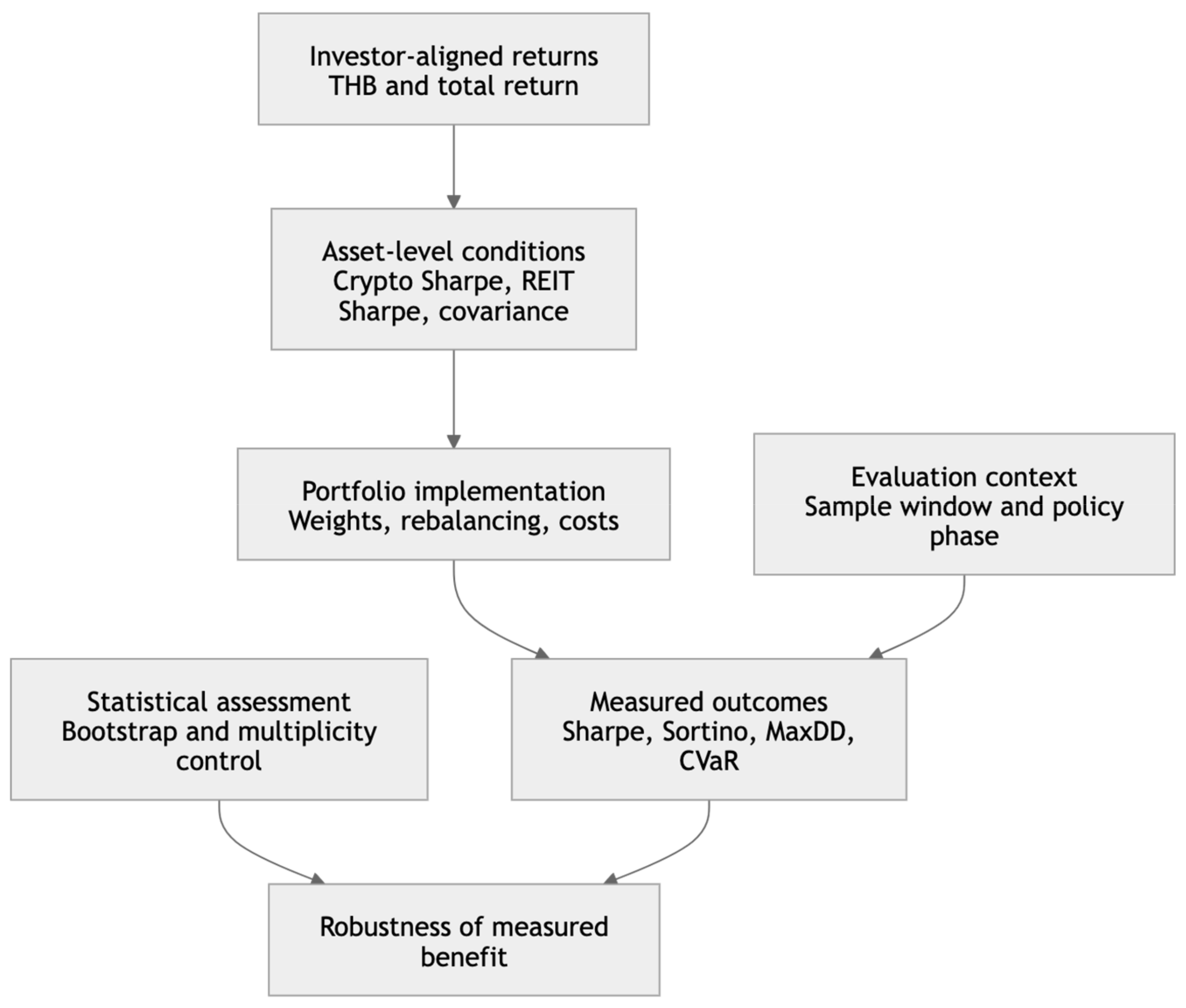
Figure 1. Conceptual framework for evaluating cryptocurrency diversification benefits in a Thai REIT portfolio.
Jrfm 19 00682 g001
Table 1. Portfolio definitions.
Portfolio REIT BTC ETH Description
P1100%Benchmark
P295%5%Fixed weight
P390%10%Fixed weight
P480%20%Fixed weight
P595%5%Fixed weight
P690%10%Fixed weight
P780%20%Fixed weight
P880%10%10%Fixed weight, mixed
P9variablevariablevariableRolling, 20% crypto cap
Target weights for P2–P8 are held at the levels above and rebalanced every 63 trading days (approximately quarterly); weights drift with realised returns between rebalancing dates. P9’s weights are re-optimised at the same 63-day frequency, over a trailing 252-day estimation window, so that at each allocation date only information available at that date is used.
Table 2. Portfolio performance, matched window (16 January 2020–30 June 2026, N = 1562).
Series/Portfolio Ann. Return Ann. Vol. Sharpe Sortino Max Drawdown Daily CVaR95
P1 REIT only−1.46%11.13%−0.192−0.226−42.9%−1.69%
P2 BTC 5%1.60%11.24%0.0830.094−31.7%−1.68%
P3 BTC 10%4.56%12.30%0.3190.364−28.5%−1.79%
P4 BTC 20%10.14%16.22%0.5980.715−29.6%−2.34%
P5 ETH 5%3.01%11.99%0.1990.226−29.9%−1.79%
P6 ETH 10%7.25%14.39%0.4700.539−31.4%−2.09%
P7 ETH 20%15.12%21.14%0.7120.874−34.6%−2.99%
P8 BTC + ETH 10/10%12.74%17.93%0.6880.807−32.2%−2.60%
P9 rolling, 20% cap16.87%18.40%0.8691.107−28.5%−2.68%
All figures are net of modelled top-level transaction costs (25 basis points per unit of two-way turnover among the REIT benchmark, Bitcoin, and Ethereum, defined below) under quarterly rebalancing; this top-level cost convention is applied identically to every portfolio, but P1’s zero modelled turnover reflects only the absence of top-level reallocation—the internal daily rebalancing within the REIT basket itself (Section 3.6) is not separately costed for any portfolio, including P1.
Table 3. ΔSharpe with 95% bootstrap confidence intervals.
Portfolio ΔSharpe 95% CI p (unadj.)p (Bonferroni)p (BH)p (Romano–Wolf)
P2 BTC 5%0.275[0.024, 0.570]0.0310.2450.0570.072
P3 BTC 10%0.511[0.035, 1.039]0.0370.2930.0570.072
P4 BTC 20%0.790[−0.028, 1.634]0.0570.4590.0590.072
P5 ETH 5%0.392[0.049, 0.808]0.0260.2100.0570.072
P6 ETH 10%0.662[0.050, 1.352]0.0340.2720.0570.072
P7 ETH 20%0.904[−0.035, 1.850]0.0590.4690.0590.072
P8 BTC + ETH0.880[0.027, 1.762]0.0420.3390.0570.072
P9 rolling1.061[0.178, 1.966]0.0230.1860.0570.038 *
ΔSharpe is the portfolio’s Sharpe ratio minus the baseline’s, with a 95% percentile interval from a moving-block bootstrap (block length 20 days, 10,000 iterations). Eight comparisons share the same benchmark; the Bonferroni-adjusted threshold is α = 0.00625. Benjamini–Hochberg and Romano–Wolf p-values are computed on the same eight-hypothesis family (Section 3.8); * denotes p < 0.05 under that method.
Table 4. Theoretical inclusion margin by year.
YearNSR(REIT)ρ (BTC)SR(BTC)Margin (BTC)ρ (ETH)SR(ETH)Margin (ETH)
2020233−1.3010.1982.0962.3540.2472.1592.480
2021241−0.5210.0051.1711.173−0.0552.1662.137
2022241−0.488−0.022−1.334−1.3450.013−0.843−0.837
2023243−1.831−0.1512.2481.973−0.0771.5961.455
20242441.3140.0591.6301.5530.0470.8470.785
20252420.9300.004−0.173−0.1770.1160.059−0.049
20261183.142−0.159−1.305−0.806−0.115−1.567−1.205
Table 5. Counterfactual ΔSharpe by target benchmark sharpe ratio.
Target SR(REIT) ΔSharpe: P4 (BTC 20%) ΔSharpe: P7 (ETH 20%)
−1.501.1741.398
−1.000.9811.153
−0.500.7880.907
0.000.5940.660
0.500.3960.409
1.000.1700.130
1.50−0.089−0.203
P9 is not recentred, since its rolling allocation would need to be re-optimised on each counterfactual series rather than simply recomputed; the counterfactual sensitivity analysis is therefore reported for the two fixed-weight portfolios only, each constructed identically to Table 2 (Section 3.5 and Section 3.6: quarterly rebalancing, weight drift, transaction costs).
Table 6. Counterfactual ΔSharpe: bootstrap confidence intervals.
Target SR(REIT)ΔSharpe (P4)95% CI (P4)p (P4)ΔSharpe (P7)95% CI (P7)p (P7)
−1.51.174[0.402, 2.019]0.006 *1.398[0.361, 2.512]0.010 *
−1.00.981[0.213, 1.821]0.014 *1.153[0.148, 2.243]0.024 *
−0.50.788[0.024, 1.622]0.043 *0.907[−0.062, 1.973]0.067
0.00.594[−0.171, 1.421]0.1290.660[−0.275, 1.702]0.164
0.50.396[−0.364, 1.216]0.3090.409[−0.518, 1.418]0.393
1.00.170[−0.578, 0.980]0.6580.130[−0.788, 1.135]0.782
1.5−0.089[−0.812, 0.759]0.847−0.203[−1.121, 0.845]0.694
* The interval excludes zero at the unadjusted 5% level. Of 14 comparisons, five exclude zero unadjusted (three for P4, at −1.5, −1.0, and −0.5; two for P7, at −1.5 and −1.0); none survives Bonferroni correction for the full family (α = 0.00357, comparable in stringency to the eight-portfolio family in Section 4.3). This comparison is therefore exploratory: it is not interpreted as family-wise significant, and the unadjusted results should be read as illustrating a pattern rather than establishing it statistically.
Table 7. Summary of nine robustness and sensitivity checks.
CheckSpecificationKey FindingEffect on Bonferroni/BH ResultTable
Excl. 2020N = 1329; SR(P1) = 0.188/8 unadj. CIs include zeroUnchanged (0/8)Table S5
Split, 1st halfN = 781; SR(P1) = −0.7666/8 unadj. exclude zeroUnchanged (0/8)Table S5
Split, 2nd halfN = 781; SR(P1) = +0.5790/8 unadj. exclude zeroUnchanged (0/8)Table S5
Block length5–60 trading daysP4/P7 sig. only at short blocks; 4 portfolios robust throughoutUnchanged (0/8)Table S3
RF level ± 25/50 bpsAll 8 portfoliosSame 6/2 unadj. split at every shiftUnchanged (0/8)Table S5B
RF timing ± 1 dayN = 1560 (fixed)P4 Δ < 0.00001P4 unchanged; other seven portfolio comparisons not re-estimatedTable S16A
After-tax (10% w/h)Uniform/quarterly lumpP4 unadj. p: 0.057 → 0.050P4 does not survive the Bonferroni threshold; the full eight-comparison family and BH adjustment were not re-estimated †Table S16B
Transaction costs0–50 bpsP9 SR: 0.884 → 0.854Rankings stableTable S2
Investable benchmarkQuarterly rebal., costedSR(P1): −0.192 → −0.112; P8 loses unadj. sig.Unchanged (0/8)Table S12
Liquidity-unscreenedSame quarterly rebal. baseSR(P1) = −0.127; same P8 changeUnchanged (0/8)Table S12
† Under the uniform-daily after-tax approximation, P4’s unadjusted p-value falls below 0.05; under the quarterly lump approximation, it lies at the 0.05 boundary. Neither result survives the Bonferroni threshold, and the full eight-comparison family and BH adjustment were not re-estimated; this does not alter the Section 4.3 conclusion, which is derived from gross returns throughout. P9’s Romano–Wolf significance (Table 3) is the only result tested for robustness across REIT-benchmark construction specifically, and survives all three (original p = 0.038, investable p = 0.048, liquidity-unscreened p = 0.046). The table lists ten rows for the nine robustness families of Section 3.9, since the sample-window family is reported as two rows (first-half, second-half) to show both halves’ results explicitly.
Disclaimer/Publisher’s Note: The statements, opinions and data contained in all publications are solely those of the individual author(s) and contributor(s) and not of MDPI and/or the editor(s). MDPI and/or the editor(s) disclaim responsibility for any injury to people or property resulting from any ideas, methods, instructions or products referred to in the content.



