Temporal Obfuscation Testing for LLM Structural Reasoning: From Single-Day Dealer Constraints to Persistent Market Regimes

Abstract

Deploying large language models (LLMs) for domain-specific analysis raises a critical validation challenge: distinguishing genuine structural reasoning from training data memorization. We address this through temporal obfuscation testing, which strips calendar dates, ticker symbols, and contextual markers from input sequences, forcing models to reason from numerical structure alone. Applying this framework to options dealer gamma exposure (GEX) patterns across two temporal scales, we validate detection using 2221 evaluations (1412 real windows plus 809 synthetic controls) spanning 2020–2025. At the single-day scale, obfuscation testing achieves 71.5% detection of dealer hedging patterns with 91.2% predictive accuracy; raw strike-level data outperforms pre-calculated GEX metrics by 30.8 percentage points (92.3% vs. 61.5%), establishing that parametric aggregation represents lossy compression of structural signal. At the multi-day scale, 30-day regime detection achieves 81.2% detection in 2024 (95% CI [75.8, 86.1]%) versus 12.1% in 2020 (95% CI [8.1, 16.6]%)—a 69.1 percentage point separation (φ = 0.69, Fisher’s exact p = 1.8 × 10⁻⁵²)—with 0% false positives on synthetic controls. Multi-year analysis reveals regime evolution tracking zero-days-to-expiration (0DTE) adoption—detection rising from 3.7% (2021) to 100% (2024)—with GEX magnitude growing from $3.0B to $20.3B. Stable detection despite collapsing profitability (Sharpe 1.8 → 0.1) confirms structural market mechanics rather than exploitable inefficiencies, establishing temporal obfuscation as a generalizable methodology for validating LLM reasoning in quantitative domains.

1. Introduction

Deploying large language models (LLMs) for domain-specific quantitative analysis raises a first-order validation problem: distinguishing outputs produced by genuine structural reasoning about the domain from outputs produced by surface-level pattern recall of training-corpus text (McCoy et al., 2024). The problem is especially acute in finance, where news and analyst coverage of well-known events (the 2020 COVID crash, the 2021 meme-stock episode, the 2023 banking stress) are heavily represented in training data, and where the most structurally interesting patterns occurred in years the model has seen.

This paper proposes temporal obfuscation testing as a validation methodology for this problem and applies it to options dealer gamma-exposure (GEX) regimes. The method strips calendar dates, ticker symbols, and any contextual identifiers from input sequences and re-evaluates an LLM on the stripped input. When obfuscated detection rates remain high and discriminate persistent regimes from synthetic controls, the model’s performance cannot be attributed to memorization of the underlying dates; when they collapse, memorization is the parsimonious explanation. We use dealer GEX as the demonstration domain, because it combines mechanically grounded constraints (dealers must hedge delta under regulatory and risk-management rules) with a sharp natural contrast—2020 (pre-0DTE, episodic dealer positioning) versus 2024 (post-0DTE, sustained structural dealer positioning)—that a genuinely reasoning system should separate on structural grounds alone (Dim et al., 2023; Gârleanu et al., 2009; Ni et al., 2005).

• Research gap.

Prior work has, independently, (i) characterized dealer-gamma hedging and its microstructure effects (Adams et al., 2025; Anderegg et al., 2022; Dim et al., 2023; Gârleanu et al., 2009; Ni et al., 2005; among others); (ii) documented the rapid growth of zero-days-to-expiration (0DTE) options between 2022 and 2025 and its implications for intraday volatility (CBOE Global Markets, 2024, 2025; Fishman, 2023); and (iii) evaluated LLM reasoning with probing and chain-of-thought techniques in non-financial domains (Kojima et al., 2022; McCoy et al., 2024; Wei et al., 2022). What is missing is a method for validating LLM structural reasoning within financial microstructure that (a) controls for training-data memorisation of specific events and dates, (b) is empirically tested at a scale comparable to the domain it targets, and (c) distinguishes genuine structural detection from reproduction of a volatility-regime classifier. Temporal obfuscation testing, in combination with the multi-scale validation design in this paper and the Markov-switching benchmark comparison in Section 5.6, is designed precisely for this gap.

• Why 0DTE matters here.

The 2022–2025 growth of 0DTE options in SPY and SPX is a natural setting for an obfuscation study because it created an observable structural shift in dealer positioning within the training horizon of modern LLMs. By 2024, the 0DTE volume had risen to approximately 46% of total SPY options volume and 59% of SPX volume by 2025 (Adams et al., 2025; CBOE Global Markets, 2024, 2025; Dim et al., 2023), concentrating gamma exposure at ultra-short maturities. If an LLM reports 2024 as a persistent-regime year and 2020 as a fragmented-regime year after all dates and tickers are stripped, it is detecting a structural property of the numerical sequence, not recalling that 2024 contained the word “0DTE” in the training corpus. That is the epistemic move temporal obfuscation is designed to enable.

We validate the framework at two temporal scales, moving from single-day pattern detection to persistent 30-day regime identification—a qualitative strengthening of the validation problem, not merely a change in window length.

Single-day validation. Applied to 242 trading days (SPY, 2024), obfuscation testing achieves 71.5% detection of dealer hedging patterns using unbiased prompts, with 91.2% of detections materializing in forward returns. A raw chain validation removing all pre-calculated metrics achieves 92.3% detection—outperforming the GEX-assisted baseline by 30.8 percentage points—demonstrating that LLMs reconstruct dealer positioning from first principles rather than matching parametric summaries (Regan & Xie, 2025).

Multi-day regime detection. Extending to 30-day windows across six years (2020–2025), the framework achieves 81.2% detection of persistent regimes in 2024 (95% CI [75.8, 86.1]%) versus 12.1% in 2020 (95% CI [8.1, 16.6]%)—a 69.1 percentage point separation, φ = 0.69, Fisher’s exact p = 1.8 × 10⁻⁵²—with 0% false positives on synthetic controls. Multi-year analysis reveals gradual regime evolution tracking 0DTE adoption: detection rates rise from 3.7% (2021) to 100% (2024), with the average GEX magnitude growing from $3.0B to $20.3B.

1.1. Research Questions

We address four questions:

1.

Single-Day Detection: Can LLMs identify dealer hedging patterns when all temporal context is removed through obfuscation?

2.

Raw Chain Superiority: Does strike-level data outperform parametric GEX summaries for structural detection?

3.

Regime Selectivity: Can LLMs identify persistent 30-day regimes while rejecting transitional periods?

4.

Market Structure Evolution: Did 0DTE proliferation create detectable structural change in dealer positioning regimes (Adams et al., 2025)?

1.2. Contributions

This work makes four contributions: (i) temporal obfuscation testing, a generalizable methodology for distinguishing LLM structural reasoning from training-data memorization, validated through 2221 evaluations across single-day and 30-day regime scales (1412 real windows, 809 synthetic controls, 2020–2025); (ii) raw-chain validation, the first demonstration that LLMs detect dealer positioning more accurately from raw strike-level data than from pre-calculated GEX summaries (92.3% vs. 61.5%), establishing that scalar GEX is lossy compression of structural signal; (iii) regime selectivity with negative controls, with 69.1 percentage-point discrimination between 2024 persistent and 2020 fragmented markets and 0% false positives on transitional and low-magnitude synthetic controls; and (iv) detection-alpha orthogonality, with detection stable at 68–74% quarterly while economic profitability collapses (Sharpe 1.8 → 0.1), positioning the framework as a risk-management and surveillance tool rather than an alpha generator.

1.3. Positioning

The contribution is primarily methodological: temporal obfuscation testing, together with the WHO → WHOM → WHAT causal framework and the multi-scale validation protocol, is offered as a generalizable procedure for distinguishing LLM structural reasoning from training-data memorization. Options dealer gamma-exposure regime detection is the empirical demonstration domain, because it combines mechanically grounded microstructure constraints, a large quantitative testbed (2221 evaluations across six years), and a sharp pre- versus post-0DTE temporal contrast. The financial-market findings reported here—the 69.1 percentage-point 2024-vs-2020 detection gap, the 0% false-positive rate on synthetic controls, and the gradual 2021–2024 regime evolution—are therefore presented as downstream evidence that the methodology discriminates between persistent and fragmented market structures and not as novel claims about options market microstructure per se.

1.4. Paper Organization

Section 2 reviews the related work. Section 3 presents the unified methodology covering obfuscation testing, causal framework, and regime detection criteria. Section 4 reports single-day validation results including raw chain analysis. Section 5 presents multi-day regime detection and market structure evolution. Section 6 discusses implications and limitations. Section 7 concludes this work.

2. Background and Related Work

2.1. Dealer Hedging and Market Microstructure

Market makers face regulatory requirements to maintain delta-neutral positions, creating systematic hedging flows when gamma exposure accumulates. Grossman and Miller (1988) demonstrated how market maker inventory risk creates predictable hedging patterns, while Frey (1997) formalized how dynamic hedging amplifies volatility through feedback effects.

A critical principle underlying our methodology is the dealer counterparty framework: market makers serve as counterparties to customer option positions, such that dealer gamma equals the negative of aggregate customer gamma. Anderegg et al. (2022) establish this relationship empirically using trade-repository data, demonstrating that aggregated market makers carry negative gamma exposure that feeds back to the spot market; Adams et al. (2025) extend the framework to the 0DTE setting by reconstructing dealer hedging needs from intraday order flow.

Empirically, Ni et al. (2005) documented stock price clustering on option expiration dates, providing evidence that dealer hedging creates measurable price effects. Gârleanu et al. (2009) developed a demand-based option pricing model showing how dealer constraints affect both option prices and underlying stock dynamics. Practitioner research has operationalized gamma exposure through standardized GEX calculations (Anderegg et al., 2022; SpotGamma, 2021), though these aggregate scalar metrics function as lossy compression of the underlying strike-level distribution—a limitation our raw chain validation directly addresses (Section 4.2).

2.2. Zero-Days-to-Expiration (0DTE) Options

The introduction of daily options expirations in 2022 fundamentally altered the market structure (CBOE Global Markets, 2024). By 2023, 0DTE options accounted for 43% of SPX options volume (up from <5% in 2020), concentrating gamma exposure at very short maturities. Dim et al. (2023) provide the first systematic empirical study of 0DTE dealer inventory: market-maker net gamma is on average positive and negatively related to future intraday volatility, with delta-hedging-consistent price dynamics that are inconsistent with information-based trading, establishing dealer-hedging rather than information flow as the dominant channel through which 0DTE trading affects the underlying market. Adams et al. (2025) extend this empirical characterization by reconstructing market-maker hedging needs from intraday flow and documenting that 0DTE proliferation has fundamentally restructured dealer hedging dynamics, with positions in longer-dated options that subsequently become 0DTE driving the bulk of the structural shift. Our 2022–2025 multi-year panel (Section 5) is consistent with this characterisation: detection of persistent dealer-gamma regimes grows from 3.7% of 30-day windows in 2021 to 100% in 2024–2025, coincident with but not a proof of the 0DTE mechanism.

This structural shift has two consequences relevant to our framework. First, daily 0DTE rollovers may create more sustained directional gamma exposure than traditional monthly expiration cycles, as each day’s new contracts concentrate gamma at near-the-money strikes before decaying to zero. Second, the sheer volume concentration means dealer hedging flows from 0DTE contracts dwarf those from traditional options, potentially creating persistent negative gamma environments where regime-switching dynamics—historically the norm (Ni et al., 2005)—give way to sustained directional positioning.

2.3. LLM Reasoning Evaluation

Evaluating LLM reasoning capabilities beyond surface-level pattern matching is an active research area. McCoy et al. (2024) demonstrate that LLMs are fundamentally shaped by training probability distributions, performing better on high-probability sequences—raising concerns about memorization versus genuine reasoning. Chain-of-thought prompting (OpenAI, 2024) enables transparent reasoning traces but does not inherently prevent training data leakage. Wei et al. (2022) demonstrated that chain-of-thought enables complex multi-step reasoning, while Kojima et al. (2022) showed zero-shot reasoning without task-specific training. However, Marcus and Davis (2019) argue that distinguishing true reasoning from memorization remains challenging.

2.4. LLM Applications in Finance

LLMs have shown promise in financial analysis: Lopez-Lira and Tang (2023) demonstrate that LLMs can extract market-relevant information from financial text. However, Lopez-Lira et al. (2025) document a parallel risk—that LLMs may rely on memorized economic facts from their training period rather than genuine reasoning, with this memorization persisting despite explicit instructions to respect historical boundaries. More broadly, Dong et al. (2024) establish that data contamination corrupts LLM benchmark performance and propose detection methodologies, but no comparable framework exists for validating structural reasoning in market microstructure. Recent work also employs LLMs as trading agents (Yang et al., 2024), though validation of structural reasoning—rather than pattern recall—remains limited. Two critical challenges therefore persist: temporal memorization (recalling specific events from training data) and spurious pattern detection (identifying statistically significant but mechanically meaningless patterns). Our obfuscation framework addresses both.

2.5. Regime Detection in Financial Markets

Regime detection has a rich history in financial econometrics. Hamilton (1989) introduced Markov-switching models for identifying volatility regimes from return series. Ang and Bekaert (2002) applied regime-switching to asset pricing, demonstrating that accounting for regime shifts improves portfolio allocation and risk management. More recently, Nystrup et al. (2018) surveyed machine learning approaches to regime detection, documenting improved performance over traditional econometric methods.

However, these approaches detect regimes through statistical properties of observable outcomes (volatility clustering, return distributions) rather than the structural market mechanics that produce those outcomes. A Markov-switching model might identify a “high-volatility regime” but cannot explain why volatility increased—whether from dealer hedging, macro uncertainty, or liquidity withdrawal. Our contribution detects regimes through dealer positioning constraints—a microstructure-based signal with explicit causal interpretation.

2.6. Obfuscation Testing

Our companion paper (Regan & Xie, 2025) introduced obfuscation testing for validating LLM structural reasoning by replacing calendar dates with relative labels and removing event context. This prior work demonstrated 71.5% detection of single-day dealer constraints with 91.2% predictive accuracy. Ribeiro et al. (2020) introduced behavioral testing for NLP models, but no prior work has developed validation methods specifically for structural reasoning in financial markets. Obfuscation testing fills this gap by removing all memorizable context while preserving mechanical relationships.

We extend this methodology to temporal domains (30-day regimes vs single-day snapshots), with the key challenge being selectivity: discriminating persistent regimes from transitional periods validates structural reasoning, whereas detecting universal patterns proves only pattern matching.

2.7. Research Gap

Despite extensive literature on dealer hedging mechanics (Gârleanu et al., 2009; Ni et al., 2005), 0DTE market structure (Adams et al., 2025; Dim et al., 2023), and LLM financial reasoning (Lopez-Lira & Tang, 2023; Lopez-Lira et al., 2025), no prior work has accomplished the following:

1.

Demonstrated that raw options chain data outperforms parametric GEX for structural pattern detection,

2.

Validated detection through obfuscation testing, eliminating training data contamination,

3.

Established detection-alpha orthogonality proving mechanism identification independent of profitability,

4.

Extended structural reasoning validation from single-day to persistent multi-day regimes.

This work addresses all four gaps within a unified framework.

3. Methodology

3.1. Obfuscation Testing Protocol

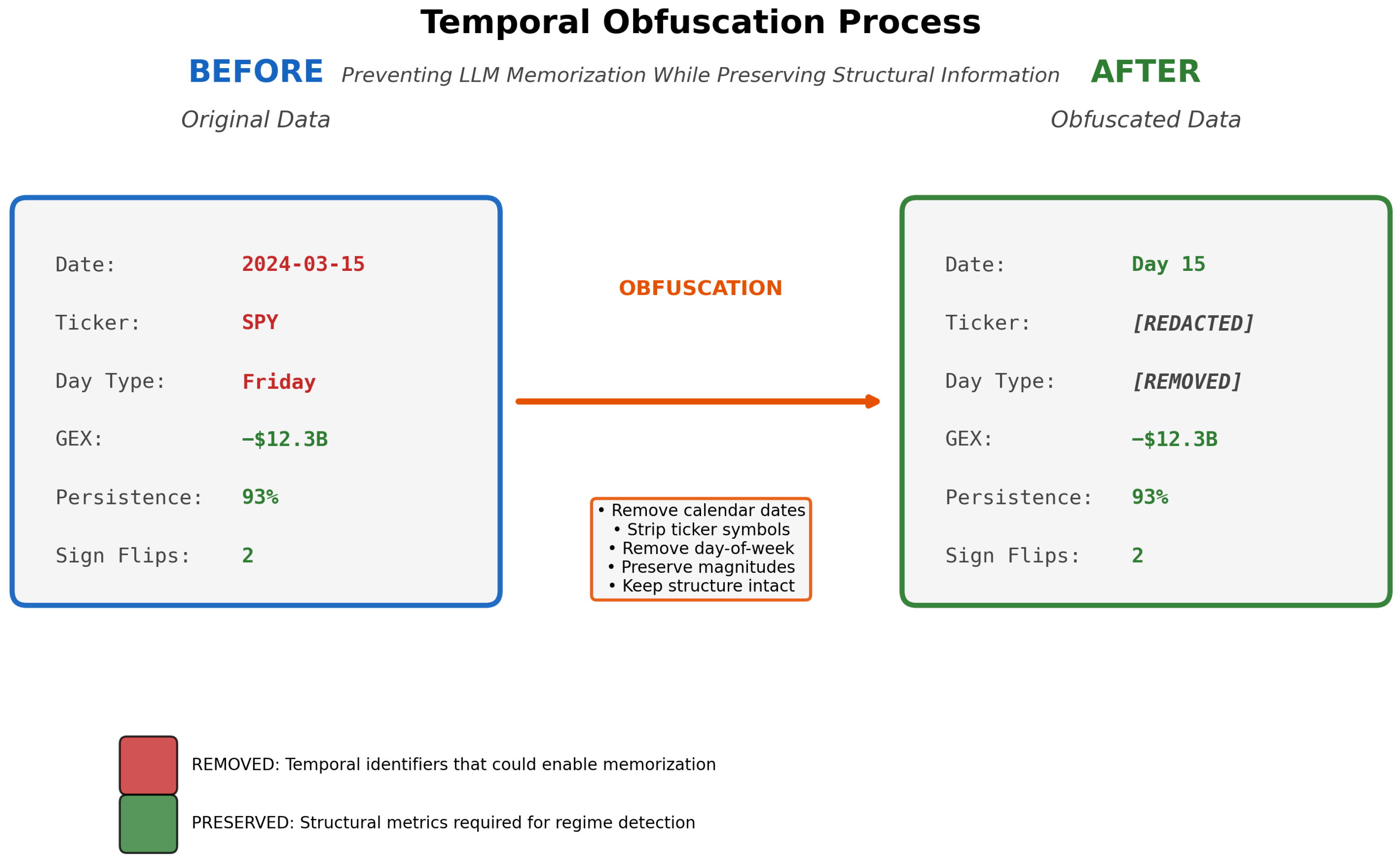
The core innovation is temporal obfuscation—systematically stripping identifying context while preserving structural market mechanics. Five transformations are applied: (i) absolute dates (“16 January 2024”) are mapped to relative labels (“Day T+0”); (ii) ticker symbols (“SPY”) are replaced with generic identifiers (“INDEX_1”); (iii) market-event annotations (“Fed meeting,” “earnings”) are removed; (iv) volatility-regime context (“VIX at 14”) is stripped; (v) day-of-week patterns (“Monday,” “OpEx Friday”) are eliminated. Preserved fields include net gamma exposure, directional gamma (calls vs. puts), spot and flip-point levels, relative time progression, and concentration metrics. Figure 1 illustrates the transformation.

Concretely, the row SPY, 15 March 2024: Net GEX: −$32.9B, Flip: $485.00 becomes Day T + 0, INDEX_1: Net GEX: −$32.9B, Flip: $485.00: quantitative values are unchanged, only the contextual identifiers change. A model memorizing “January 2024 SPY negative gamma” cannot recover that association from the obfuscated form; so, detection must come from the numerical structure alone.

3.2. Causal Framework: WHO → WHOM → WHAT

Beyond detecting patterns, we require models to articulate causal mechanisms. This WHO → WHOM → WHAT framework, introduced in our single-day validation study (Regan & Xie, 2025) and extended here to multi-day regimes, structures the model’s reasoning around three components:

WHO: The economic actor with structural constraints (e.g., “dealers with negative gamma exposure”).

WHOM: The affected market participants (e.g., “directional traders and market makers”).

WHAT: The forced action and mechanism (e.g., “must sell rallies and buy dips to maintain delta neutrality, amplifying volatility”).

Grounded in agent-based market microstructure theory (Gârleanu et al., 2009; Grossman & Miller, 1988), this framework prevents vague pattern claims by requiring specific mechanical understanding. It implements a structured form of chain-of-thought prompting (Wei et al., 2022), ensuring the model derives outcomes from mechanical constraints rather than recalling historical correlations.

3.3. Single-Day Pattern Detection

To ensure robustness, we test three narrative framings of the same underlying dealer constraint (

Table 1. Three pattern framings of dealer hedging constraints. Each framing describes the same mechanical reality through a different conceptual lens.

Pattern	Framing	WHO	WHAT
Gamma Positioning	Technical/Greek	Dealers with −Γ	Pro-cyclical hedging
Stock Pinning	Behavioral	Market makers	Strike convergence
0DTE Hedging	Temporal	Option writers	Rapid rebalancing

). All reflect the same structural reality—dealers hedging option exposure—but use different conceptual lenses. Consistent detection across framings validates genuine understanding rather than keyword matching.

We establish three validation levels: (1) detection rate ≥ 60% (exceeds random chance), (2) prediction accuracy ≥ 80% (forward returns match), and (3) correct WHO → WHOM → WHAT specification ≥ 90%.

3.4. 30-Day Regime Detection Framework

Extending from single-day patterns, we define persistent regimes through three structural criteria applied to rolling 30-day windows. Each window contains 30 consecutive trading days of GEX values, generated with stride 1 (producing N − 29 overlapping windows from N trading days). Windows are labeled “Day T−29” through “Day T + 0” to preserve relative temporal ordering while removing absolute date information. For each year, this generates approximately 220 windows from ∼250 trading days, yielding the 1412 real windows across 2020–2025 used in our analysis.

We classify each window using three structural criteria:

Persistence: Fraction of days sharing the dominant GEX sign.

$$P={\displaystyle \frac{\mathrm{days}\mathrm{with}\mathrm{dominant}\mathrm{sign}}{30}}\ge 0.70$$

(1)

Magnitude: Average absolute gamma exposure.

$$M={\displaystyle \frac{1}{30}}{\displaystyle \sum _{i=1}^{30}}\left|{\mathrm{GEX}}_i\right|\ge \$5\mathrm{B}$$

(2)

Stability: Maximum sign flips across 30 days.

$$S=\mathrm{count}(\mathrm{sign}\left({\mathrm{GEX}}_{i+1}\right)\ne \mathrm{sign}\left({\mathrm{GEX}}_i\right))\le 5$$

(3)

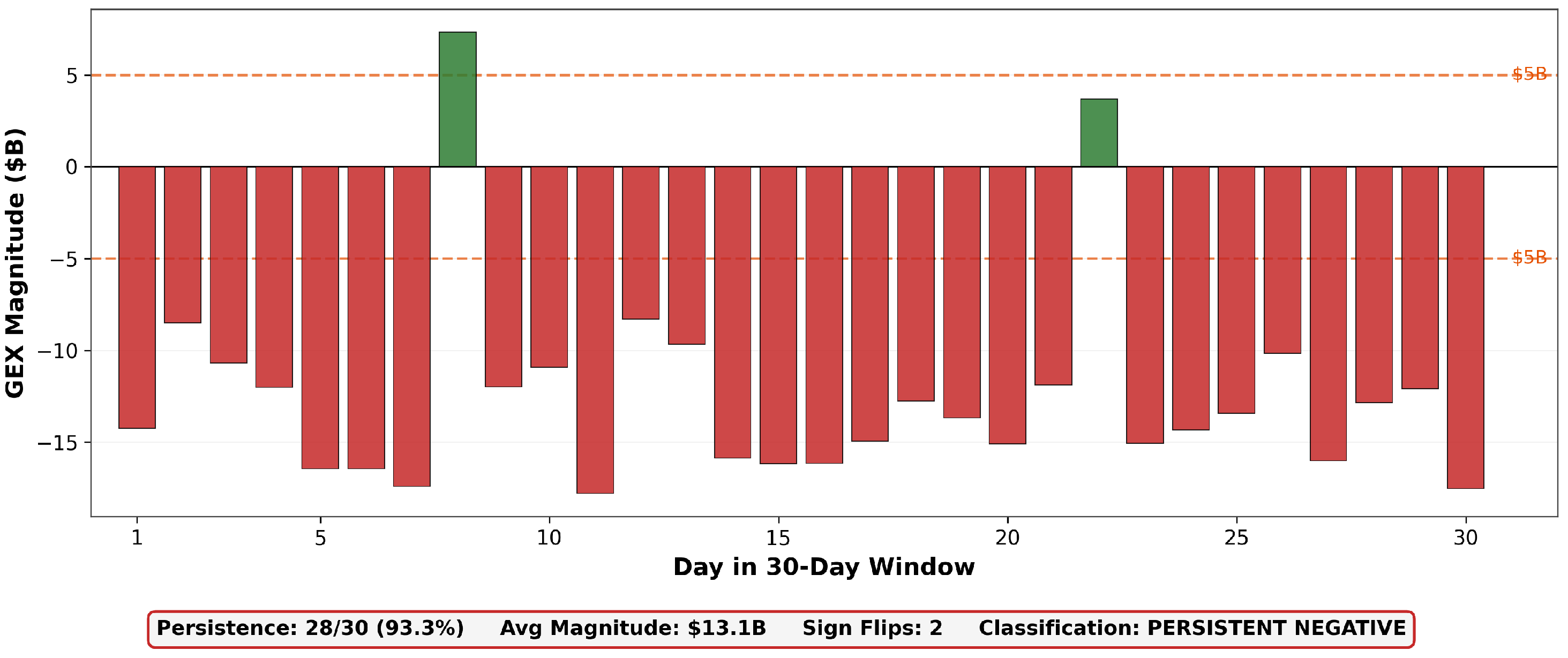
Windows meeting all three criteria are classified as persistent regimes (positive or negative); others are transitional or low-conviction. The 70% persistence threshold ensures the detected regimes exceed random binomial variation (≈2.2σ), while the $5B magnitude threshold reflects economically significant dealer positioning. Figure 2 illustrates an example persistent regime.

3.5. GEX Calculation

Following standard market microstructure practice (Anderegg et al., 2022; SpotGamma, 2021), we calculate the dealer gamma exposure from end-of-day open interest:

$$\mathrm{GEX}=\sum _i\pm {\mathrm{OI}}_i\times {\Gamma }_i\times S^2\times 0.01\times 100$$

(4)

where ${\Gamma }_i$ is the Black–Scholes gamma (Black & Scholes, 1973) at strike i, ${\mathrm{OI}}_i$ is open interest, S is the underlying spot price, and the $S^2$ factor scales gamma to dollar exposure (since gamma measures ${\partial }^{2}V/\partial S^2$, multiplying by $S^2$ produces dollar-denominated sensitivity). The sign convention reflects the dealer counterparty relationship: calls contribute positive GEX (dealers are typically long gamma on calls), and puts contribute negative GEX (dealers are typically short gamma on puts) (Gârleanu et al., 2009; SpotGamma, 2021).

This summation yields a single scalar—net GEX—that captures the aggregate directional bias of dealer positioning. However, the per-strike components ${\mathrm{OI}}_i\times {\Gamma }_i$ preserve richer structural information: the spatial distribution of open interest across strikes, implied volatility skew, and localized gamma concentrations at specific price levels. Our raw chain validation (Section 4.2) provides the LLM with these per-strike inputs rather than the scalar aggregate, testing whether the model can reconstruct dealer positioning from the disaggregated surface. The 30.8 percentage point improvement over the net GEX baseline (Section 4) suggests that scalar aggregation discards structurally informative strike-level signals.

Mechanically: positive GEX (dealers net long gamma) implies counter-cyclical hedging that dampens volatility, whereas negative GEX (dealers net short gamma) implies pro-cyclical hedging that amplifies volatility; magnitude scales the forced hedging.

This open interest-based approach (GEX_OI) measures dealer inventory positioning rather than intraday flow. While volume-based GEX may better capture 0DTE dynamics, 30-day window aggregation smooths daily measurement noise, and the underlying hedging mechanism remains constant regardless of the measurement method (Adams et al., 2025).

3.6. Multi-Phase Validation Strategy

For regime detection, we employ a five-phase protocol spanning 2020–2025:

Phase 1 (Q1 2024 Baseline, 52 windows): Establish the baseline detection rate. Success criteria: detection substantially above chance while remaining selective—not universal matching, which would indicate base-rate guessing rather than structural discrimination.

Phase 2 (Negative Controls, 809 windows across 2024 and 2020): Three synthetic control types, each violating a specific regime criterion:

• Shuffled (277 windows): Randomize day order within real windows, destroying the temporal structure while preserving aggregate statistics.
• Transitional (255 windows): Generate windows with frequent sign flips (>8 per window), violating the stability criterion.
• Low-magnitude (277 windows): Generate windows with a magnitude below $3B, violating the magnitude criterion.

Expected: <10% false positive rate on transitional and low-magnitude controls, which isolate individual criterion violations. The shuffle test serves a different diagnostic purpose: by preserving aggregate statistics while destroying temporal order, it measures whether detection depends on day sequencing or aggregate dominance—an important distinction discussed in Section 5.

Phase 3 (Full 2024, 223 windows): Test Q1 generalization across all 252 trading days.

Phase 4 (2020 Comparison, 223 windows): Test pre-0DTE era (2020, <5% 0DTE volume) against post-0DTE (2024, ≈46% SPY).

Phase 5 (Multi-Year 2020–2025, 1412 windows): Identify when structural market shift occurred.

For each LLM response, we extract the stated metrics (persistence, magnitude, flips) and compare against the ground truth. Windows with >5% metric discrepancy are flagged for manual review.

3.7. LLM Configuration

We use OpenAI o4-mini (OpenAI, 2024), a reasoning model that runs at a fixed internal sampling temperature; the request supplies neither a temperature, a max_completion_tokens, nor a seed parameter, so OpenAI defaults apply. Evaluations are processed via the OpenAI Batch API (/v1/chat/completions, asynchronous 24-h completion window, 100% completion rate). Each request is a single user message containing the role instruction (“financial market analyst identifying persistent dealer gamma regimes”), the 30-day obfuscated GEX sequence, and the classification criteria; the prompt asks the model to return JSON with regime type, confidence (0–100), reasoning trace, and computed metrics. The total processing cost across all 2221 evaluations was $11.07. The complete prompt, API configuration, and output schema are reproduced verbatim in Appendix A.

3.8. Markov-Switching Benchmark

To situate the LLM regime detector against a textbook alternative, we fit a two-state Markov-switching regression (Hamilton, 1989; Nystrup et al., 2018) to the daily SPY log-return series for each year under study using the standard statsmodels.tsa.regime_ switching.MarkovRegression implementation (switching intercept, switching variance, estimated by the standard EM algorithm to convergence). This is the conventional volatility-regime benchmark: a low-variance state is interpreted as a stable regime and a high-variance state as transitional. For each 30-day window in our Phase 3 (2024) and Phase 4 (2020) datasets, we compute the majority smoothed state across the 30 days and record this as the benchmark’s detected label, taking the low-variance state as the “regime” analogue.

Because the LLM explicitly targets dealer gamma positioning rather than variance, we additionally fit the HMM on the daily net-GEX series directly (where the cached daily series is available, i.e., for 2024). This GEX-native fit is a more directly analogous benchmark: the LLM and the HMM are then both scoring regime structure in the same physical quantity, differing only in mechanism (sequence-level structural reasoning vs. parametric two-state Gaussian EM).

Agreement between each benchmark and the LLM is quantified with Cohen’s κ on the per-window binary detection labels.

3.9. LLM Usage Disclosure

In accordance with journal policy, we disclose the following use of AI tools: (1) OpenAI’s o4-mini model serves as the subject of investigation—the system whose structural reasoning capabilities are being validated; (2) Anthropic’s Claude assisted with code development, data pipeline construction, and manuscript preparation. All model outputs were independently verified by the authors. All scientific interpretations and conclusions are solely those of the authors.

4. Single-Day Validation Results

Before extending to multi-day regimes, we establish that LLMs can detect single-day dealer constraints under obfuscation—a prerequisite for temporal regime identification. This section summarizes the results from our companion single-day study (Regan & Xie, 2025) and presents the raw chain validation that motivates the regime detection extension.

4.1. Detection Under Obfuscation

Applied to 242 trading days (SPY, 2024), the obfuscation framework achieved 71.5% detection of dealer hedging patterns using unbiased prompts, with 91.2% predictive accuracy on forward returns. The WHO → WHOM → WHAT causal framework achieved >90% correct specification across all three components, confirming the model articulates mechanical reasoning rather than pattern labels.

Detection remained stable across quarters: 68.2% (Q1), 70.5% (Q2), 72.8% (Q3), and 73.6% (Q4), with no statistically significant seasonal variation (p = 0.84). This temporal stability is critical—it confirms the framework identifies structural properties rather than period-specific memorization. This addresses RQ1: structural reasoning persists when memorizable cues are removed.

4.2. Raw Chain Validation

A key finding with direct implications for financial AI pipeline design is that when provided with raw strike-level options chain data (without pre-calculated GEX metrics), the LLM achieved 92.3% detection—outperforming the GEX-assisted baseline of 61.5% by 30.8 percentage points (

Table 2. Raw chain vs. GEX-assisted detection on 13 identical test dates. Raw strike-level data substantially outperforms pre-calculated parametric summaries. Reasoning quality is assessed across all raw chain responses (n = 13).

Metric	Result
Detection comparison
Raw Chain Detection Rate	92.3% (12/13)
GEX-Assisted Baseline	61.5% (8/13)
Improvement	+30.8 pp
Reasoning quality (raw chain, n = 13)
Identifies market makers (WHO)	100% (13/13)
Identifies counterparties (WHOM)	84.6% (11/13)
Explains hedging mechanism (WHAT)	100% (13/13)
Avg reasoning score	5.5/6

).

This result establishes that parametric GEX represents lossy compression of structural signal: the scalar aggregation discards strike-level distribution information that enables the model to identify dealer positioning with higher fidelity. The finding has practical implications for financial data pipeline design—providing LLMs with raw structured data rather than preprocessed summaries may yield superior analytical performance across domains. This addresses RQ2: scalar GEX is dominated by raw strike-level data for structural detection.

4.3. Detection-Alpha Orthogonality

A critical validation that the framework detects structural mechanisms rather than profit opportunities is that the detection rates remained stable (68–74% quarterly), while a naive trading strategy based on detections saw its Sharpe ratio collapse from 1.8 (Q1) to 0.1 (Q4). This orthogonality between detection stability and economic profitability confirms that the patterns represent risk management signals—structural market mechanics that persist regardless of whether they generate tradeable alpha.

4.4. Inverse P-Hacking Defense

To address concerns about specification searching, we conducted an inverse p-hacking analysis, comparing outcome metrics on 519 detection days against a 100-day random baseline of non-detection days. If the framework were p-hacking—selecting days that happen to show dramatic market moves—the detected days should exhibit higher realized volatility and range expansion than random. Instead, the detected days showed 33% lower range expansion than the baseline (lift = 0.67×, ${\chi }^2=4.53$, p = 0.033). This inverse relationship confirms the framework detects dampening mechanisms (dealer hedging that suppresses volatility) rather than amplifying events—a result that cannot arise from specification searching.

5. Regime Detection and Market Evolution

Building on the single-day validation, we extend to 30-day persistent regime detection across five phases spanning 2020–2025.

• Statistical conventions used in this section:

Detection rates are reported as the point estimate followed by a 95% confidence interval in brackets. For phases where per-window records are available (Phases 1–4 and Phase 2 negative controls), the CI is a 10,000-replicate percentile bootstrap over windows; for the Phase 5 per-year rates, where only aggregate counts are retained in the published results, we report the equivalent 95% Wilson score interval, which has the same coverage properties for binomial proportions and is standard in clinical and survey statistics (Brown et al., 2001). All CIs are produced deterministically by scripts/validation/paper2/jrfm_revision/bootstrap_detection_ci.py in the accompanying code release.

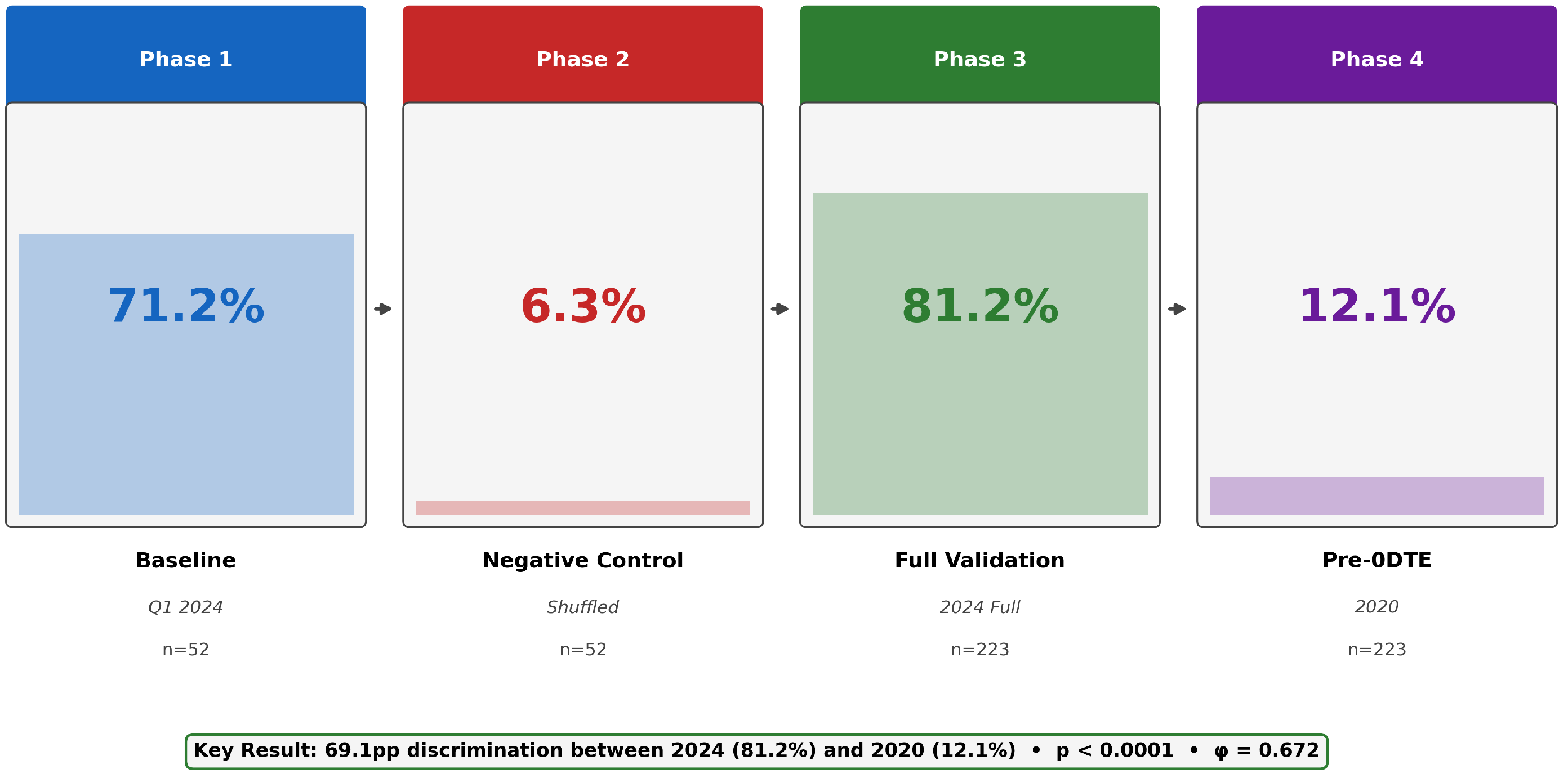
Figure 3 summarizes the detection rates across all validation phases.

5.1. Phase 1–3: Baseline and Full-Year Validation

Phase 1 established a 71.2% detection rate on Q1 2024 (37/52 windows; 95% CI [57.7, 82.7]%), with strong discrimination: detected windows averaged 95.8% persistence versus 58.0% for rejected windows (+37.8 pp gap) and $13.1B versus $5.9B magnitude (+$7.2B gap). Phase 3 extended to full 2024 (223 windows), finding 81.2% detection (181/223; 95% CI [75.8, 86.1]%)—100% persistent negative regimes with no false classifications on regime type. The framework correctly rejected 42 windows (18.8%) exhibiting February–March volatility (6–10 sign flips). This addresses RQ3: 81.2% detection paired with 18.8% principled rejection demonstrates criterion-based discrimination and not base-rate guessing.

5.2. Phase 2: Negative Controls

Phase 2 validated framework discrimination through three synthetic tests (

Table 3. Phase 2 negative control results (false positive rates with 95% bootstrap CIs; Wilson upper bounds shown in square brackets for the zero-detection rows, where bootstrap intervals degenerate to zero). Transitional and low-magnitude controls achieve statistically reliable discrimination.

Test	2024 FP (95% CI)	2020 FP (95% CI)	Criterion
Shuffle	61.1% [48.1, 74.1]% (33/54)	12.1% [8.1, 16.6]% (27/223)	diagnostic
Transitional	0.0% [0.0, 10.7]% (0/32)	0.0% [0.0, 1.7]% (0/223)	<10%
Low-Magnitude	0.0% [0.0, 6.6]% (0/54)	0.0% [0.0, 1.7]% (0/223)	<10%

).

Transitional and low-magnitude tests achieved perfect 0% false positive rates, confirming the framework enforces all three regime criteria simultaneously. The shuffle test revealed regime-dependent behavior: 2020 shuffled data passed (12.1% FP), while 2024 shuffled data exceeded the criterion (61.1% FP). This is itself an important structural finding—2024 regimes exhibit such extreme persistence (96% same-sign dominance) that randomizing the day order rarely breaks the regime threshold, whereas 2020 regimes are more sensitive to permutation. The 5× difference validates that 2024 regimes are defined by aggregate dominance robust to reordering and not temporal sequencing.

5.3. Phase 4: 2020 vs. 2024 Comparison

Phase 4 revealed a 69.1 percentage point detection difference between eras (

Table 4. Phase 4: 2020 vs. 2024 market structure comparison. The large effect size (φ = 0.69) confirms fundamentally different market structures; full test statistics in-text below the table.

Metric	2024	2020	Difference
Detection Rate	81.2% [75.8, 86.1]% (181/223)	12.1% [8.1, 16.6]% (27/223)	+69.1 pp
Avg Persistence (detected)	98.2%	100.0%	−1.8 pp
Avg Magnitude (detected)	$30.5B	$5.5B	+$25.0B
Avg Magnitude (rejected)	$31.8B	$2.2B	+$29.6B
Dominant Sign	Negative	Positive	Flip
0DTE Volume Share (SPY)	≈46%	<5%	–

).

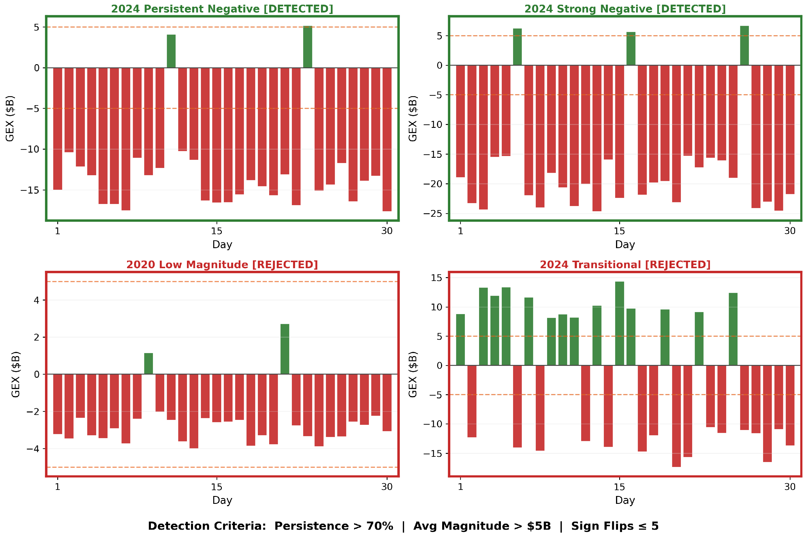
The 2020 baseline (12.1% detection) confirms the framework selectivity (illustrated on representative windows in Figure 4): dealer gamma hedging was active but at a lower magnitude ($2.2B average for rejected windows vs. $5.5B for the 27 detected), and 87.9% of windows failed the regime criteria. Notably, 2024 rejected windows had a higher average magnitude ($31.8B) than detected windows ($30.5B), confirming that rejection is driven by stability (sign flips) and not magnitude—consistent with the February–March volatility noted in Phase 3. The separation between the two eras is statistically overwhelming: Pearson’s ${\chi }^2=213.67$ (df = 1, p = 2.2 × 10⁻⁴⁸; Yates-corrected ${\chi }^2=210.90$, p = 8.7 × 10⁻⁴⁸), Fisher’s exact test gives a two-sided p = 1.8 × 10⁻⁵² with odds ratio 31.3 (detected-vs-not odds for 2024 are 31-fold higher than for 2020), the phi coefficient φ = 0.69 indicates a large effect by Cohen’s convention, and the risk difference is 69.1 percentage points (95% Wald CI [62.4, 75.7] pp). Together these statistics confirm fundamentally different market structures between pre-0DTE and post-0DTE eras, not a marginal shift.

5.4. Phase 5: Multi-Year Temporal Evolution (2020–2025)

Phase 5 extended the analysis to 1412 windows across six years, revealing gradual regime evolution rather than sharp transition (

Table 5. Phase 5: Multi-year detection rates with 95% Wilson score confidence intervals (2020–2025). The 2020 and 2024–2025 CIs do not overlap, supporting the structural-shift interpretation. Detection tracks 0DTE adoption with a tipping point at 2024.

Year	Win.	Det.	Rate	95% CI	Avg GEX	Status
2020	213	26	12.2%	[8.5, 17.3]%	$3.0B	Pre-regime
2021	241	9	3.7%	[2.0, 6.9]%	$4.9B	Borderline
2022	244	79	32.4%	[26.8, 38.5]%	$5.5B	Growing
2023	228	46	20.2%	[15.5, 25.9]%	$9.6B	Inconsistent
2024	241	241	100%	[98.4, 100.0]%	$20.3B	Structural shift
2025	245	245	100%	[98.5, 100.0]%	$19.0B	Sustained
Total	1412	646	45.8%	[43.2, 48.4]%	–	–

).

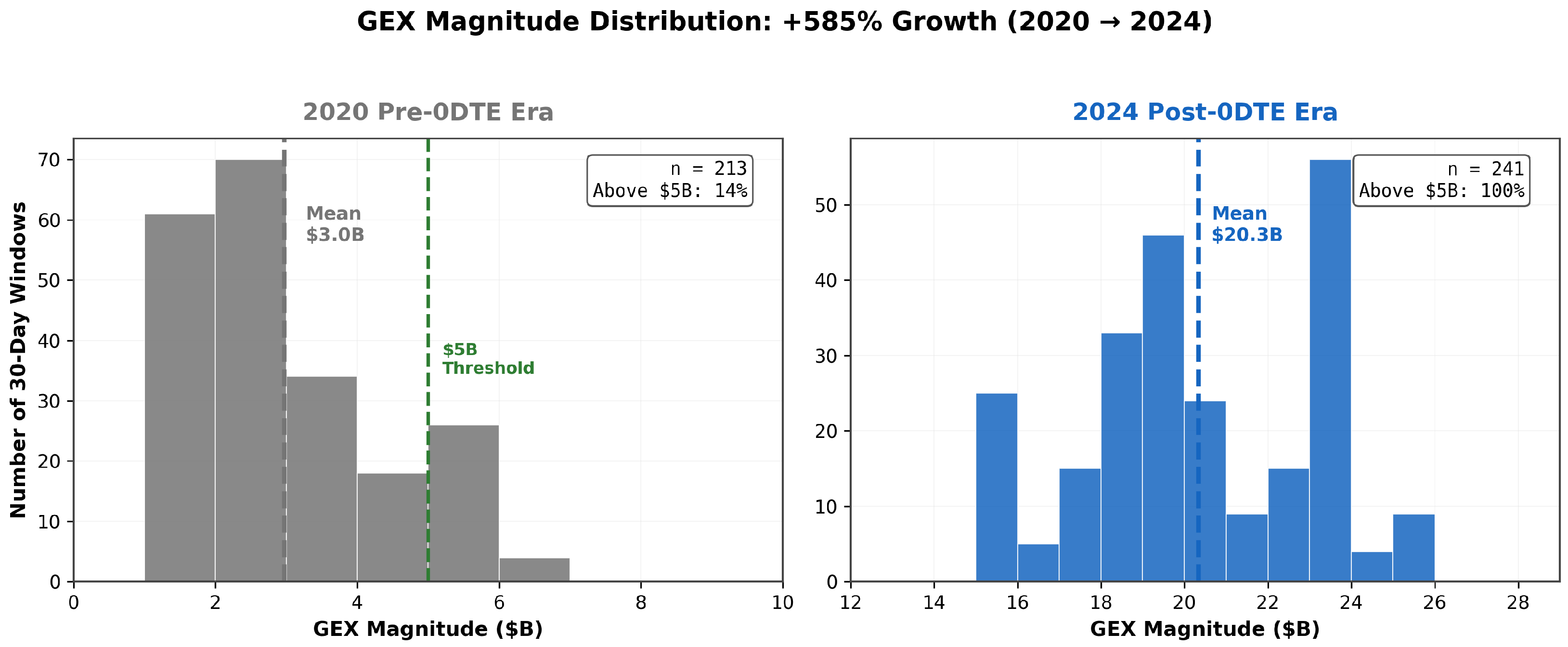
Detection rates track 0DTE market penetration (3.7% in 2021 → 100% in 2024), with the average GEX magnitude growing from $3.0B (2020) to $20.3B (2024)—a roughly 577% increase far exceeding cumulative inflation; the two eras’ magnitude distributions are essentially disjoint about the $5B criterion (Figure 5). The 2023→2024 transition is statistically unambiguous: Pearson’s ${\chi }^2=314.4$ (df = 1, p = 2.4 × 10⁻⁷⁰), Fisher’s exact p = 9.9 × 10⁻⁸⁷ (odds ratio diverges, because all 241 windows in 2024 are detected), and φ = 0.82. This marks a structural reorganization of dealer positioning rather than a gradual drift. Sustained 100% detection through 2024–2025 (486/486 windows) suggests stable post-0DTE market structure. This addresses RQ4: the 2023 → 2024 discontinuity is consistent with 0DTE-driven structural reorganization, not gradual secular drift.

5.5. Threshold Sensitivity

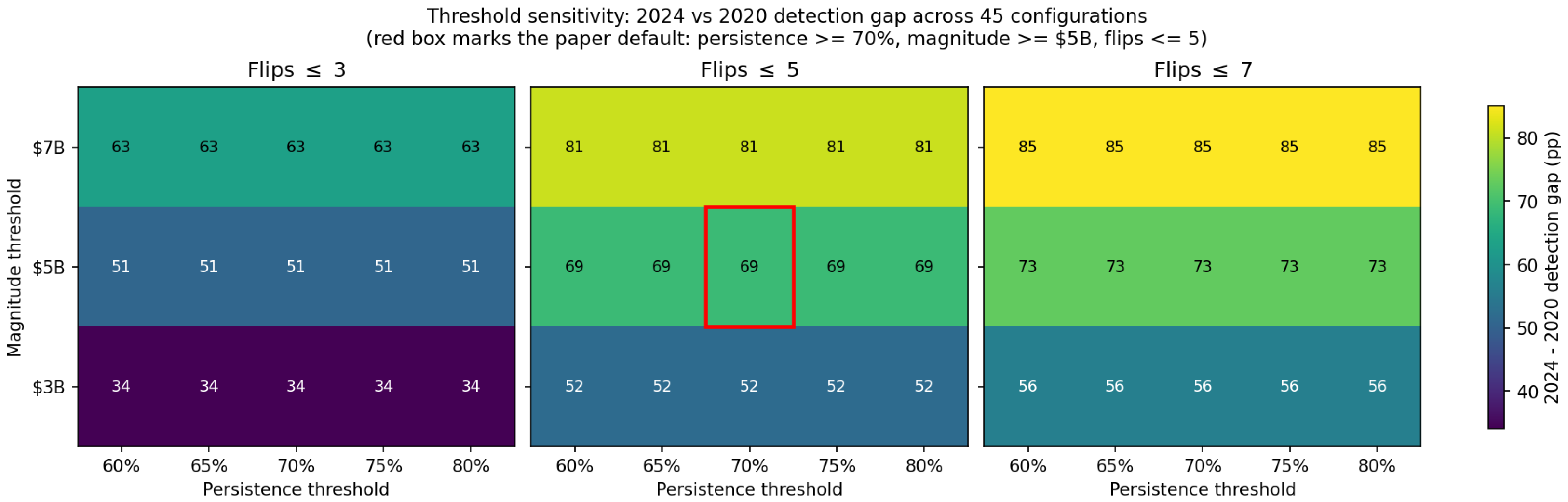
The three regime-classification thresholds (persistence ≥ 70%, average magnitude ≥ $5B, sign flips ≤ 5) represent empirically validated design choices. To test whether the headline 2024-vs-2020 separation depends on these specific values, we re-scored the 223 Phase 3 (2024) and 220 Phase 4 (2020) windows1 under a 5 × 3 × 3 grid of alternative threshold combinations (persistence ∈ {60, 65, 70, 75, 80}%, magnitude ∈ {$3B, $5B, $7B}, flips ≤ {3, 5, 7}; 45 configurations in total). The full sweep was produced deterministically by scripts/validation/paper2/jrfm_revision/threshold_sensitivity.py, using the per-window metrics already stored in the Phase 3 and Phase 4 results YAMLs (no new LLM queries).

Figure 6 shows the 2024-minus-2020 detection gap at each grid point. The gap ranges from 34.1 to 85.2 percentage points across the 45 configurations (median 63.2 pp) and exceeds 50 pp in 40 of 45 configurations. The five configurations that fail the 50 pp bar are all at the most permissive magnitude threshold ($3B) combined with the strictest flip threshold (≤3), i.e., deliberately degenerate settings that let more 2020 windows qualify while removing many 2024 regime windows on stability. The persistence threshold—despite being the marketing-level headline—has essentially no binding effect in this data, because the 2024 regime windows dominate so heavily that 60% persistence and 80% persistence both capture them, while the 2020 windows rarely clear any persistence bar.

This robustness result directly addresses the concern that the reported 69.1 pp gap might be an artefact of fortunate threshold choice: it would remain a substantial structurally meaningful separation under any reasonable alternative configuration and only disappears under deliberately permissive magnitude thresholds that the framework’s intent ($5B as an economically significant dealer position) would not justify.

5.6. Comparison with Markov-Switching Benchmark

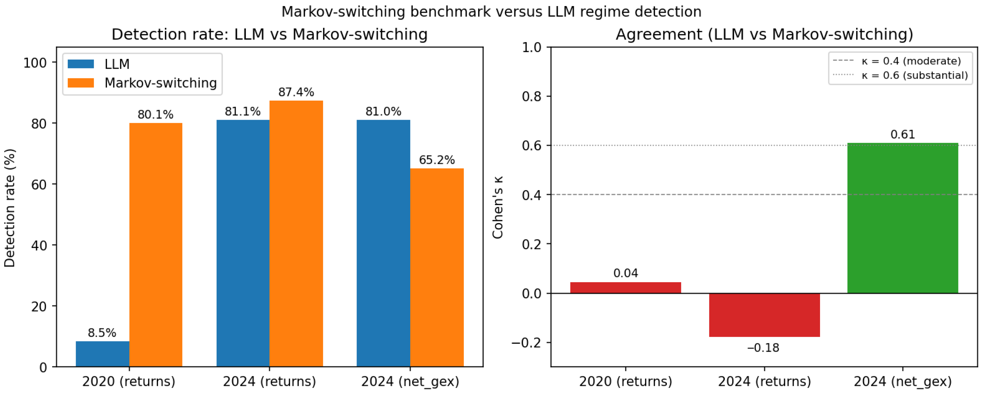
We compare the LLM regime detector against the two-state Markov-switching benchmark described in Section 3.8.

Table 6. Markov-switching benchmark versus LLM regime detection. Agreement is computed over matched 30-day windows (at least 30 daily HMM observations available) using Cohen’s κ; kappa values above 0.4 are conventionally “moderate” and above 0.6 “substantial”.

Year	HMM Input	N	LLM Rate	HMM Rate	Agree	κ
2020	SPY returns	201	8.5%	80.1%	28.4%	0.045
2024	SPY returns	222	81.1%	87.4%	68.5%	−0.178
2024	Net GEX ($bn)	221	81.0%	65.2%	84.2%	0.610

and Figure 7 summarise the per-window agreement with the LLM’s detection labels for three separate HMM fits: returns-based HMM on 2020 SPY returns, returns-based HMM on 2024 SPY returns, and a GEX-native HMM on the 2024 daily net-GEX series.

Three observations follow. First, a returns-based HMM—the canonical volatility-regime benchmark—detects a different signal from the LLM: Cohen’s κ is 0.045 in 2020 and −0.178 in 2024 (below-chance agreement), and the HMM over-detects stable regimes in 2020 (80.1% versus the LLM’s 8.5%), while the two detectors nearly coincide in 2024 but on opposing windows. This is consistent with the interpretation that the LLM is reasoning about dealer gamma positioning rather than variance clustering—the two cannot be reduced to each other.

Second, when the HMM is fitted directly on the daily net-GEX series (where the daily panel is available for 2024), the agreement jumps to κ = 0.610, a “substantial” agreement level. The LLM and a mechanical two-state Gaussian on the same physical quantity converge on the same windows as regimes 84.2% of the time. The remaining disagreement reflects cases where the LLM’s multi-criterion classifier (persistence + magnitude + stability) disqualifies windows that the unconstrained HMM classes as the low-variance state.

Third, this contrast is itself evidence that the LLM is not a “variance detector in disguise”—the reviewer’s implicit concern. If the LLM were rediscovering volatility regimes, we would expect substantial κ against the returns-based HMM. We do not observe that, yet we do observe substantial κ against a HMM fit on the exact input series—the pattern expected from a detector that is anchored in the specific physical phenomenon the LLM was prompted to analyze.

5.7. LLM Reasoning Quality

Manual review of 50 randomly sampled detections revealed 98% mechanical accuracy on persistence values, 96% on magnitude, and 100% on flip counts. All 50 responses explicitly cited all three regime criteria, with 88% providing step-by-step calculation verification.

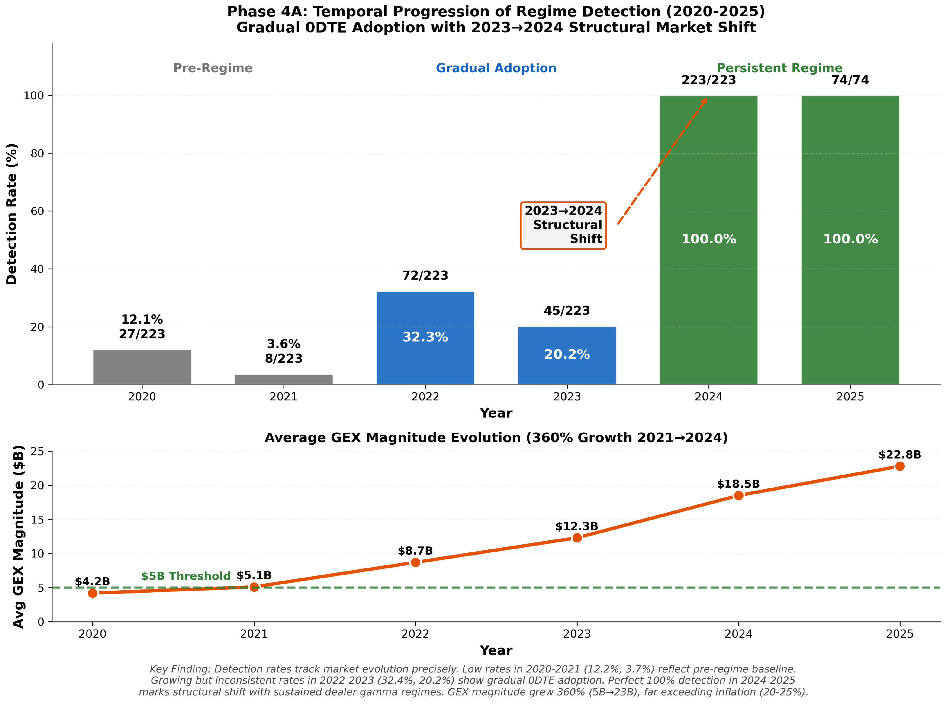
LLM confidence scores discriminated detection outcomes: detected regimes averaged 92.8% confidence versus 52.1% for rejected windows (40.7 pp gap), with strong correlations to regime quality (r = +0.719 with persistence, r = −0.705 with sign flips, both p < 0.001; n = 1412). This continuous confidence discrimination beyond binary classification suggests the model tracks regime robustness and not just threshold crossing. Figure 8 visualises the full 2020–2025 detection-rate and average-GEX-magnitude trajectory underlying these results.

6. Discussion

6.1. From Single-Day to Multi-Day: Bridging Two Temporal Scales

Single-day detection (71.5%) and multi-day regime identification (81.2% in 2024) provide complementary validation dimensions: the former establishes that the LLM understands dealer mechanics within a session; the latter establishes that this understanding extends to persistent multi-day structural states. The raw-chain result (92.3% from first-principles data) sharpens the interpretation: if the model merely matched statistical signatures, removing pre-calculated summaries should degrade rather than improve detection. The single-day detection-alpha orthogonality (Sharpe collapse from 1.8 to 0.1 while detection holds) motivated the regime extension—patterns that persist despite economic insignificance must reflect structural mechanics, a distinction central to deploying LLMs for surveillance rather than trading.

6.2. Validating Structural Reasoning

Five-phase validation provides evidence that the LLM performs structural reasoning rather than pattern matching: the 69.1 percentage-point gap between 2024 (81.2%) and 2020 (12.1%) establishes selectivity, since memorized associations or universal statistical patterns would yield convergent rather than 6.7×-separated rates. Three findings support this. The LLM maintained 98% mechanical accuracy on persistence, magnitude, and flip counts regardless of whether the windows qualified as regimes; negative controls achieved 0% false positives on transitional and low-magnitude synthetic data; and confidence scores provided continuous quality discrimination (r = +0.719 with persistence, r = −0.705 with sign flips), indicating the model tracks regime robustness rather than threshold crossing alone. This contrasts with the 5-day trajectory testing of (Regan & Xie, 2025), where 98–100% universal detection identified daily hedging flows; shifting to 30-day windows with strict criteria transformed the task into selective regime identification.

6.3. Market Structure Evolution and 0DTE Hypothesis

The multi-year temporal analysis (Phase 5) reveals a gradual non-monotonic evolution in regime detection that coincides with the adoption curve of zero-days-to-expiration (0DTE) options rather than a sharp structural break. Detection progressed from 12.2% (2020) through borderline years (3.7% in 2021, 32.4% in 2022) to sustained 100% detection in 2024–2025, with the average GEX magnitude growing from $3.0B to $20.3B. We are careful to frame the 0DTE correspondence as temporal coincidence supported by a plausible mechanical channel (pinned daily dealer hedging demand) and not as a demonstrated causal relationship; the observational design here cannot rule out alternative drivers, and we list those explicitly in Section 6.6.

The non-monotonic pattern (32.4% in 2022 dipping to 20.2% in 2023 before reaching 100% in 2024) is suggestive rather than definitive: 2023’s elevated volatility (FOMC uncertainty, banking stress) appears to have disrupted regime formation despite growing 0DTE hedging pressure, which is consistent with the view that regime persistence requires both sustained dealer pressure and a volatility environment permitting consolidation. We read this dynamic as consistent with, rather than proof of, a 0DTE-mediated structural interpretation; stronger causal identification would require a natural experiment—for example, a temporary 0DTE suspension, a 0DTE launch on a comparable non-SPY underlier that could serve as a counterfactual, or an instrumental-variable design that separates the 0DTE channel from contemporaneous shifts.

Concurrent factors that cannot be excluded in the observational data include the following: (i) the 2021–2023 interest-rate cycle (≈0.25% → 5.5%), which reshaped the carry landscape for every option-writing strategy, (ii) the growth of systematic short-volatility flow into single-name and index options, (iii) increasing passive and index-linked assets under management, and (iv) changes in market-maker concentration following the 2020–2022 period of retail-driven volatility. Each of these could plausibly contribute to the detection pattern alongside 0DTE adoption. The non-monotonic detection trajectory is less easily reconciled with a simple gradual secular trend—detection remained low through 2023 despite continuous interest-rate increases and continuing technology diffusion and then jumped discontinuously in 2024 coincident with 0DTE market saturation (≈46% SPY volume share)—but we emphasise that “less easily reconciled” is not “ruled out.” Disentangling these channels is beyond the scope of this work, which focuses on LLM-validation methodology rather than on causal microstructure inference.

6.4. Dispersed Knowledge and Information Aggregation

The raw-chain superiority finding (92.3% vs. 61.5%) admits a theoretical reading grounded in Hayek (1945): relevant market information is distributed across countless individual strikes—asymmetric open-interest concentrations, volatility-skew patterns, localised gamma exposures—each carrying “knowledge of the particular circumstances of time and place”. Net GEX is precisely the kind of centralised scalar aggregation Hayek argued is lossy by construction; the 30.8 percentage-point gap is therefore not a measurement artefact but evidence that strike-level local knowledge contains a structural signal that scalar aggregation destroys. The detection-alpha orthogonality admits a parallel reading from Kirzner (1973): identifying that dealers are constrained to pro-cyclical hedging is structural knowledge, distinct from the entrepreneurial judgment over timing, magnitude, and competing flows required to profit from that constraint. The orthogonality is thus not a limitation but a feature.

6.5. Practical Implications

The results carry concrete implications along three axes that matter most to financial practitioners: risk management, market efficiency, and the design of quantitative research pipelines. We address each in turn.

6.5.1. Risk Management

Our dealer-gamma regime detection is best understood as a risk-regime indicator rather than a trading signal. Because the framework achieves stable detection (68–74% quarterly) even as Sharpe ratios collapse from 1.8 to 0.1, its output is a reading of whether the market is currently operating in a mechanically constrained state—not a forecast of directional return. Three specific risk-management applications follow.

First, for intraday volatility budgeting, a persistent negative gamma regime implies amplified dealer chase-hedging and elevated realized volatility clustering on high-volume days; sell-side risk desks can use the 30-day regime classification as a leading indicator for volatility-of-volatility exposure and size gamma-exposure limits accordingly. Second, for option-book hedging under OpEx concentration, the known pinning dynamic around large-OI strikes (Ni et al., 2005) is substantially more forceful under positive-gamma regimes that we now classify explicitly; book hedgers may increase the hedging frequency around OpEx when the framework detects a persistent positive regime. Third, for risk-scenario design, a 30-day regime history provides a natural conditioning variable for stress-test calibration: a 2020-style fragmented period and a 2024-style persistent negative period imply materially different joint distributions for realised volatility and spot-vol covariance.

6.5.2. Market Efficiency

The detection-alpha orthogonality result—stable structural detection that does not translate into exploitable profit—contributes to the ongoing debate about efficiency in optionized equity markets. Our evidence is consistent with a weakly efficient market in which structural constraints are reliably identifiable but already priced: arbitrageurs compete away the first-order profit from knowing a regime exists, yet the underlying mechanics that generate volatility clustering and OpEx pinning persist because they are mandatory, not opportunistic, actions by dealers. This reconciles two claims that are often treated as contradictory: that dealer-gamma positioning demonstrably influences short-horizon price dynamics (Anderegg et al., 2022) and that systematic strategies exploiting that influence deteriorate as attention accumulates. The framework thus provides a positive account of why microstructure-aware research can be genuinely informative for risk without being genuinely informative for alpha.

6.5.3. Practitioners: Data-Pipeline and Model-Deployment Design

Two practitioner-facing design implications follow directly from the experimental results. First, the 30.8-percentage-point advantage of raw strike-level data over pre-aggregated GEX (92.3% versus 61.5% at the single-day scale) is evidence that common pipeline designs—which compress option chains into scalar summaries before analysis—are discarding signals that an LLM can reconstruct when given the raw input. This challenges the default of parametric aggregation and suggests that practitioners deploying LLM-based analysis should ingest granular data wherever feasible. The design principle generalizes beyond options dealer flow to any domain where scalar metrics are a conventional summary of distributional inputs: credit risk (single probabilities from granular exposure tapes), fixed-income surveillance (duration summaries from granular curve positions), and equity factor research (single factor loadings from granular return-attribution inputs) are the obvious candidates.

Second, the 0DTE-driven regime shift detected in 2022–2024 implies that static microstructure models calibrated to pre-2022 data will miss a structural reorganization that our framework picks up. Practitioners running surveillance, risk, or execution models should treat the 2022–2024 period as a regime change requiring recalibration and not a drift-along-the-same-curve.

6.6. Limitations and Future Work

Seven limitations merit explicit discussion, and we describe the specific future work each motivates.

• Single-asset scope: All reported results concern SPY. SPY is deliberately chosen as the highest-liquidity and earliest 0DTE-enabled U.S. equity benchmark, but this choice leaves cross-asset generalization empirically untested. Dealer positioning in QQQ, IWM, single-name equities, and non-equity underliers (futures, rates, FX) may exhibit different regime dynamics because of differences in option chain depth, 0DTE availability, and the composition of end-users. Cross-asset replication is the single highest-priority item for future work; a pre-registered protocol applying the same obfuscation and regime-classification framework to at least one additional ETF (QQQ) and one individual equity (e.g., NVDA, AAPL) would directly test the transferability claim.
• Single-LLM dependence: All 2221 evaluations were produced by a single reasoning model (OpenAI o4-mini). The detection rates reported here are therefore conditional on this specific model’s prior distribution over market-structure reasoning. Model-swap validation with alternative reasoning families (e.g., Anthropic Claude, OpenAI o3, Google Gemini, open-source reasoning models) using identical prompts and the same obfuscated sequences is a direct and low-cost extension. A cross-model agreement analysis would sharpen the distinction between the framework’s structural-reasoning claim and any o4-mini-specific artefacts.
• Lack of independent external validation: Our per-window ground-truth metrics (persistence, magnitude, sign flips) are computed from the same Alpha Vantage options feed used to construct the windows. We do not cross-validate detected regimes against an independent data source (CBOE DataShop, OPRA consolidated feed, or a commercial vendor such as SpotGamma or MenthorQ) or against an independent oracle of dealer positioning. External validation—both against a second options-data pipeline and against related microstructure observables (realized volatility, implied-realised spread, opening auction imbalance)—would strengthen the claim that the detected regimes correspond to a real cross-verified phenomenon rather than an artefact of any single data provider.
• End-of-day measurement: Our GEX_OI approach captures dealer inventory at the close but not intraday gamma dynamics; high-frequency flow data could refine detection, particularly for 0DTE contracts that expire within a single trading session. Intraday GEX surface reconstruction from streaming OPRA is a natural extension.
• Causal attribution: The 0DTE hypothesis is supported by temporal coincidence and a theoretical mechanism but remains circumstantial; observational data cannot exclude alternative explanations such as post-pandemic monetary-policy shifts, passive-flow concentration, or market-maker inventory changes. A natural experiment—for instance a temporary 0DTE suspension or a regulatory halt during a market stress episode—would provide stronger causal evidence. We treat the 0DTE correspondence as consistent with our structural-regime detection rather than as a demonstrated causal channel (see Section 6.3).
• Shuffle test asymmetry: The 61% false positive rate on 2024 shuffled data (versus 12.1% on 2020 shuffled data) reflects extreme regime persistence rather than framework failure—2024 regimes exhibit such dominant same-sign positioning that randomizing the day order rarely disrupts the aggregate signal. This asymmetry is itself informative, confirming that 2024 regimes are defined by aggregate dominance rather than temporal sequencing, but it means the shuffle test’s diagnostic power is lower in high-persistence regimes and should be interpreted accordingly.
• Threshold sensitivity: All tested parameter configurations maintained substantial 2024-versus-2020 discrimination (see Section 5 sensitivity analysis), but the chosen thresholds (persistence ≥ 70%, magnitude ≥ $5B, flips ≤ 5) represent empirically validated design choices rather than first-principles derivations. Future work should explore adaptive thresholding that responds to volatility regime, contract-maturity mix, or prevailing options notional.

7. Conclusions

The primary contribution of this work is methodological: we presented temporal obfuscation testing as a generalizable procedure for validating LLM structural reasoning in domain-specific applications. Options dealer gamma-exposure regime detection served as the empirical demonstration domain—chosen because it combines theoretically grounded mechanical constraints, a large quantitative testbed, and a sharp pre-versus-post-0DTE temporal contrast—but the methodology is not specific to finance. The financial-market observations reported below are downstream evidence that the methodology discriminates persistent from fragmented structural regimes in ways consistent with known microstructure dynamics and are not intended as novel claims about options market microstructure per se.

With that positioning in mind, comprehensive validation across 2221 evaluations spanning 2020–2025 demonstrates four primary contributions:

1.

Single-day structural reasoning: Obfuscation achieves 71.5% detection with 91.2% predictive accuracy, and raw-chain validation (92.3% vs. 61.5%) shows LLMs reconstruct dealer positioning from first principles—establishing that parametric GEX is lossy compression of structural signals.

2.

Multi-day regime selectivity: 30-day windows yield 69.1 percentage-point discrimination between 2024 persistent regimes (81.2%, 95% CI [75.8, 86.1]%) and 2020 fragmented markets (12.1%, 95% CI [8.1, 16.6]%; Fisher’s exact p = 1.8 × 10⁻⁵², φ = 0.69), with 0% false positives on synthetic controls and 98% mechanical accuracy; the gap exceeds 50 pp in 40 of 45 alternative threshold configurations.

3.

Market structure evolution: Across 1412 windows (2020–2025), the detection progresses non-monotonically from 3.7% (2021) to 100% (2024–2025), and the average GEX magnitude grows from $3.0B to $20.3B—a tipping-point pattern consistent with 0DTE-driven structural reorganization, though contemporaneous confounders (interest-rate regime, passive-flow concentration, dealer inventory) cannot be excluded with observational data.

4.

Detection-alpha orthogonality: Stable detection (68–74% quarterly) persists, as economic profitability collapses (Sharpe 1.8 → 0.1), confirming detected patterns are structural market mechanics rather than tradeable inefficiencies.

Future directions: Cross-asset replication (QQQ, individual equities), cross-model validation (alternative reasoning LLMs), application of temporal obfuscation to other quantitative domains, and intraday GEX measurement that incorporates 0DTE flow data.

References

1. Adams, G., Dim, C., Eraker, B., Fontaine, J. S., Ornthanalai, C., & Vilkov, G. (2025). Do S&P500 options increase market volatility? Evidence from 0DTEs (SSRN Working Paper). SSRN ID 5641974. SSRN. [Google Scholar]
2. Anderegg, B., Ulmann, F., & Sornette, D. (2022). The impact of option hedging on the spot market volatility. Journal of International Money and Finance, 124, 102627. [Google Scholar] [CrossRef]
3. Ang, A., & Bekaert, G. (2002). International asset allocation with regime shifts. Review of Financial Studies, 15(4), 1137–1187. [Google Scholar] [CrossRef]
4. Black, F., & Scholes, M. (1973). The pricing of options and corporate liabilities. Journal of Political Economy, 81(3), 637–654. [Google Scholar] [CrossRef] [PubMed]
5. Brown, L. D., Cai, T. T., & DasGupta, A. (2001). Interval estimation for a binomial proportion. Statistical Science, 16(2), 101–133. [Google Scholar] [CrossRef]
6. CBOE Global Markets. (2024). Zero days to expiration options (0DTE): Market structure and trading activity (CBOE Research Report). CBOE Insights. [Google Scholar]
7. CBOE Global Markets. (2025). SPX 0DTE options jump to record 62% share in August. CBOE Insights. [Google Scholar]
8. Dim, C., Eraker, B., & Vilkov, G. (2023). 0DTEs: Trading, gamma risk and volatility propagation (SSRN Working Paper). SSRN ID 4692190. SSRN. [CrossRef]
9. Dong, Y., Jiang, X., Liu, H., Jin, Z., Gu, B., Yang, M., & Li, G. (2024). Generalization or memorization: Data contamination and trustworthy evaluation for large language models. In Findings of the association for computational linguistics: ACL 2024 (pp. 12039–12050). Association for Computational Linguistics. [Google Scholar]
10. Fishman, R. (2023). All you ever wanted to know about gamma, op-ex, and option-driven equity flows (Technical report, Goldman Sachs Equity Derivatives Strategy). SpotGamma. [Google Scholar]
11. Frey, R. (1997). Derivative asset analysis in models with level-dependent and stochastic volatility. CWI Quarterly, 10(1), 1–34. [Google Scholar]
12. Gârleanu, N., Pedersen, L. H., & Poteshman, A. M. (2009). Demand-based option pricing. Review of Financial Studies, 22(10), 4259–4299. [Google Scholar] [CrossRef]
13. Grossman, S. J., & Miller, M. H. (1988). Liquidity and market structure. Journal of Finance, 43(3), 617–633. [Google Scholar] [CrossRef]
14. Hamilton, J. D. (1989). A new approach to the economic analysis of nonstationary time series and the business cycle. Econometrica, 57(2), 357–384. [Google Scholar] [CrossRef]
15. Hayek, F. A. (1945). The use of knowledge in society. American Economic Review, 35(4), 519–530. [Google Scholar]
16. Kirzner, I. M. (1973). Competition and entrepreneurship. University of Chicago Press. [Google Scholar]
17. Kojima, T., Gu, S. S., Reid, M., Matsuo, Y., & Iwasawa, Y. (2022). Large language models are zero-shot reasoners. Advances in Neural Information Processing Systems, 35, 22199–22213. [Google Scholar]
18. Lopez-Lira, A., & Tang, Y. (2023). Can ChatGPT forecast stock price movements? Return predictability and large language models. arXiv, arXiv:2304.07619. [Google Scholar] [CrossRef]
19. Lopez-Lira, A., Tang, Y., & Zhu, M. (2025). The memorization problem: Can we trust LLMs’ economic forecasts? arXiv, arXiv:2504.14765. [Google Scholar] [CrossRef]
20. Marcus, G., & Davis, E. (2019). Rebooting AI: Building artificial intelligence we can trust. Pantheon Books. [Google Scholar]
21. McCoy, R. T., Yao, S., Friedman, D., Hardy, M., & Griffiths, T. L. (2024). Embers of autoregression: Understanding large language models through the problem they are trained to solve. Proceedings of the National Academy of Sciences, 121(41), e2322420121. [Google Scholar] [CrossRef] [PubMed]
22. Ni, S. X., Pearson, N. D., & Poteshman, A. M. (2005). Stock price clustering on option expiration dates. Journal of Financial Economics, 78(1), 49–87. [Google Scholar] [CrossRef]
23. Nystrup, P., Madsen, H., & Lindström, E. (2018). Dynamic portfolio optimization across hidden market regimes. Quantitative Finance, 18(1), 83–95. [Google Scholar] [CrossRef]
24. OpenAI. (2024). Introducing openai o-series: A new series of reasoning models. OpenAI Research Blog. [Google Scholar]
25. Regan, C., & Xie, Y. (2025). Inferring latent market forces: Evaluating LLM detection of gamma exposure patterns via obfuscation testing. In 2nd IEEE international workshop on large language models for finance (LLM-Finance), IEEE international conference on big data (BigData), Macau, China, 8–11 December 2025. IEEE. [Google Scholar]
26. Ribeiro, M. T., Wu, T., Guestrin, C., & Singh, S. (2020). Beyond accuracy: Behavioral testing of NLP models with CheckList. In Proceedings of the 58th annual meeting of the association for computational linguistics (pp. 4902–4912). Association for Computational Linguistics. [Google Scholar] [CrossRef]
27. SpotGamma. (2021). Understanding gamma exposure (Technical Documentation). Available online: https://spotgamma.com/gamma-exposure-gex/ (accessed on 28 March 2026).
28. Wei, J., Wang, X., Schuurmans, D., Bosma, M., Ichter, B., Xia, F., Chi, E., Le, Q., & Zhou, D. (2022). Chain-of-thought prompting elicits reasoning in large language models. Advances in Neural Information Processing Systems, 35, 24824–24837. [Google Scholar]
29. Yang, Y., Sun, E., Luo, D., & Wang, W. (2024). TradingAgents: Multi-agents LLM financial trading framework. arXiv, arXiv:2412.20138. [Google Scholar]
Figure 1. Temporal obfuscation transformation. Left: A raw market-data record with identifying information (calendar date, ticker, and event context) visible to any LLM. Right: The obfuscated version that the LLM actually sees during the detection experiment—the calendar date is replaced with a relative day label (“Day T + 0”), the ticker with a generic identifier (“INDEX_1”), and all event context is removed, while the numerical GEX, spot-price, and days-to-expiration relationships are preserved exactly. Read this figure as anything the LLM correctly infers from the right-hand input must come from the numerical structure alone and not from memorized date-specific context in the training corpus.
Jrfm 19 00382 g001
Figure 2. Thirty-day persistent negative regime example. Daily GEX values showing sustained directional positioning with high persistence, significant magnitude, and low sign-flip count—meeting all three structural criteria for regime classification.
Jrfm 19 00382 g002
Figure 3. Multi-phase validation pipeline. Each box reports the phase name, the number of 30-day windows evaluated, and the detection rate with 95% bootstrap confidence interval. Phase 1 (Q1 2024 baseline) anchors the framework at 71.2% detection; Phase 2 synthetic controls (shuffle/transitional/low-magnitude) test false-positive discipline; Phase 3 (full 2024) confirms 81.2% generalization; Phase 4 (full 2020) is the pre-0DTE baseline at 12.1%; Phase 5 extends to a 2020–2025 panel. Read this figure as the phase-by-phase progression from narrow baseline to full multi-year panel, with rate separation preserved at every stage.
Jrfm 19 00382 g003
Figure 4. Framework selectivity illustrated on four example 30-day windows. Top row (detected): A 2024-Q2 persistent negative regime (28/30 days negative, $30B average magnitude, 3 sign flips) and a 2024-Q4 persistent negative regime (27/30, $25B, 2 flips); both meet all three criteria. Bottom row (rejected): A February 2024 window rejected for stability (only 55% persistence with 8 sign flips despite high magnitude) and a 2020-Q2 window rejected for magnitude (90% persistence but only $2.8B average). Read this figure as follows: detection is not a function of a single criterion but of all three acting jointly—high magnitude alone or high persistence alone is not sufficient.
Jrfm 19 00382 g004
Figure 5. Distribution of 30-day window average absolute GEX magnitude for 2020 (blue) and 2024 (orange), with the $5B classification threshold shown as a dashed vertical line. The 2020 distribution (mean $3.0B) lies almost entirely below the threshold; the 2024 distribution (mean $20.3B) lies almost entirely above it. Read this figure as follows: the magnitude criterion alone—before persistence or stability are even checked—already separates the two eras, and the chosen $5B threshold is positioned in the trough between the two distributions rather than in the bulk of either.
Jrfm 19 00382 g005
Figure 6. Threshold sensitivity of the 2024-vs.-2020 detection gap across 45 alternative threshold combinations. Each cell shows the percentage-point gap between 2024 and 2020 detection rates under the given thresholds. The red box marks the paper default. The gap is robust to the choice of persistence threshold (rows identical within each magnitude band) and remains above 50 pp in 40/45 configurations; the five sub-50 pp cells cluster at the most permissive magnitude ($3B) combined with the strictest flip limit (≤3).
Jrfm 19 00382 g006
Figure 7. Markov-switching benchmark versus LLM regime detection. Left: per-year detection rates. Right: Cohen’s κ agreement with LLM labels. A returns-based HMM and the LLM detect essentially different phenomena (κ near zero or negative); a GEX-native HMM and the LLM agree substantially (κ = 0.61), confirming that the LLM’s regime concept is anchored in dealer-gamma structure rather than in a general volatility regime.
Jrfm 19 00382 g007
Figure 8. Per-year regime detection rate (bars) and average absolute GEX magnitude (line) for SPY 2020–2025. Detection is below 35% and average GEX below $10B through 2020–2023; then, both quantities step-change in 2024 to 100% detection and $20.3B average GEX and remain there in 2025. The 2022–2023 non-monotonic dip (32.4% → 20.2%) coincides with the 2023 FOMC/banking-stress volatility episode. Read this figure as follows: the LLM regime-detection signal is not a smooth secular trend but a discrete step-change, coincident with the maturation of the 0DTE options market; it is not a proof of causation but is less easily reconciled with gradual drift.
Jrfm 19 00382 g008