Improving Ethereum Price Forecasting Through Hybrid Decomposition and LSTM–Attention Mechanisms

Abstract

This study investigates the predictive performance of decomposition-based deep learning models through a focused case study on Ethereum price forecasting. Using hourly Ethereum price data from 5 September 2020 to 13 July 2025, we develop hybrid forecasting frameworks that integrate three signal decomposition techniques—Wavelet Decomposition (WD), Variational Mode Decomposition (VMD), and Empirical Mode Decomposition (EMD)—with a Long Short-Term Memory network enhanced by an attention mechanism (LSTM–Attention). The decomposition methods are first applied to extract multiple frequency components from the original time series, allowing the forecasting model to capture both short-term fluctuations and long-term dynamics inherent in this specific digital asset. Each decomposed component is then modeled using the LSTM–Attention architecture, and the forecasts are aggregated to produce the final prediction. The predictive performance of the proposed models is evaluated using MAE, MSE, RMSE, and MAPE, and the results are compared with benchmark models including ARIMA-GARCH and standard LSTM–Attention. Forecast accuracy is assessed through out-of-sample one-step-ahead predictions, and robustness is ensured by averaging results across 10 independent runs. The empirical results demonstrate that incorporating decomposition techniques substantially improves forecasting accuracy. Among the tested models, the EMD–LSTM–Attention framework achieves the best performance, producing the lowest forecasting errors. While focused on the Ethereum market, these findings highlight the effectiveness of combining signal decomposition and attention-based deep learning architectures to enhance predictive performance in high-volatility cryptocurrency environments.

1. Introduction

Time-series forecasting plays a vital role in decision-making across several domains, including finance, energy, and the social sciences (Kolambe & Arora, 2024). In financial markets, forecasting variables such as asset prices and market indicators is often a complex process that requires multiple modeling attempts and iterative refinements before reliable predictions can be achieved. However, the nonstationary and nonlinear nature of financial data significantly complicates time-series forecasting (Y. Liu et al., 2022). In recent years, advanced data modeling techniques based on machine learning have substantially improved forecasting accuracy, overcoming some of the limitations associated with traditional statistical methods. Among these techniques, attention-based long short-term memory (LSTM) networks have gained considerable attention due to their ability to identify relevant historical patterns and assign adaptive weights to important past observations.

Recent studies on attention-based deep learning models, particularly recurrent neural network architectures such as Long Short-Term Memory (LSTM) combined with attention mechanisms, have demonstrated strong performance in financial time series forecasting. These models enhance predictive accuracy by allowing the network to focus on the most relevant past observations and temporal patterns when modeling nonlinear and nonstationary financial data. Consequently, attention-based forecasting frameworks have become increasingly effective in capturing complex time-series dynamics across multiple temporal scales (Zhou et al., 2021). Signals in time series data are linked to the interactions of events across both long and short time periods. The attention unit supplements the main LSTM by modulating its outputs to capture the evolving volatility and underlying dynamics of input data sequences. The attention mechanism improves predictive performance by allowing models to focus on the most relevant information during the learning process (Abbasimehr & Paki, 2021). By assigning different weights to past observations, attention-based models can capture important temporal dependencies more effectively than traditional LSTM models (Ladhari & Boubaker, 2024). While the integration of LSTM–Attention models has advanced the field, the existing literature often treats the input signal as a singular entity, which can lead to information loss when the data contains highly heterogeneous noise levels. As noted by Zhou et al. (2021), the challenge of long-sequence time-series forecasting lies in capturing the dependencies within extremely long histories without succumbing to the high complexity and memory usage that can obscure signal clarity. Prior hybrid approaches have begun exploring signal decomposition; however, many studies rely on a single decomposition method without accounting for the specific strengths and weaknesses of different signal-processing techniques (Zheng et al., 2020). There remains a critical gap in understanding which decomposition–attention framework most effectively isolates the predictive signal from the high-frequency noise inherent in cryptocurrency markets.

Building on these developments, the present study contributes to this literature by integrating and comparatively evaluating three distinct signal decomposition techniques (wavelet decomposition, Variational Mode Decomposition, and Empirical Mode Decomposition) with an LSTM–Attention forecasting framework. Unlike prior studies that focus on a single hybrid architecture (Aswadi & Ependi, 2025). this research provides a robust empirical framework to determine how different decomposition physics interact with attention mechanisms to capture multi-scale temporal dynamics in the highly volatile Ethereum market.

Despite these advantages, LSTM–Attention models also present certain limitations. In some cases, the architecture may become overly complex when attempting to capture intricate temporal patterns embedded in financial time series, which may affect predictive performance and risk management applications (Wang et al., 2021). Although attention mechanisms allow the model to automatically assign weights to relevant inputs, the architecture may suffer from overfitting when the available dataset is limited, thereby reducing its generalization capability.

Furthermore, deep learning models often require extensive data preprocessing and denoising to remove irrelevant information before training. This preprocessing stage may increase computational complexity and complicate the practical implementation of LSTM–Attention models in real-world financial forecasting tasks. In addition, the training process can be computationally expensive, particularly when dealing with highly stochastic and nonlinear financial data, which require the model to learn complex temporal dependencies across long sequences (Zheng et al., 2020).

Another important challenge arises from the non-stationary nature of financial time series. Non-stationarity refers to structural changes in the statistical properties of a series over time, which can significantly affect forecasting applications such as cryptocurrency price prediction or asset price volatility forecasting. In cryptocurrency markets, these distributional shifts often occur due to sudden market crashes, regulatory announcements, technological developments, or periods of extreme volatility that alter the underlying dynamics of price movements. Ignoring non-stationarity may lead to biased model estimation and unreliable forecasts (Ryan et al., 2023). Consequently, addressing non-stationary behavior is essential for improving predictive performance in financial markets.

To address these challenges, recent studies suggest integrating signal decomposition techniques with deep learning architectures. Decomposition methods allow complex time series to be separated into simpler components representing different temporal frequencies or patterns. In this study, three decomposition techniques—Wavelet Decomposition (WD), Variational Mode Decomposition (VMD), and Empirical Mode Decomposition (EMD)—are combined with the LSTM–Attention model to better capture multi-scale structures and reduce the impact of noise and non-stationarity in financial data. By decomposing the original time series into multiple components, the proposed framework improves the model’s ability to learn hidden patterns and enhances forecasting accuracy in cryptocurrency markets.

The main contributions of this study can be summarized as follows. First, we develop hybrid forecasting models that integrate three decomposition techniques (WD, VMD, and EMD) with an attention-based LSTM architecture to better capture complex patterns in financial time series. Second, we conduct a comprehensive comparative analysis of these hybrid models to evaluate their effectiveness in forecasting Ethereum prices. Third, the empirical results demonstrate that the EMD–LSTM–Attention model achieves superior predictive performance across several evaluation metrics, highlighting the benefits of combining decomposition techniques with deep learning models for financial forecasting.

The remainder of this paper is organized as follows. Section 2 reviews the related literature. Section 3 describes the methodology and evaluation metrics. Section 4 presents the dataset and empirical results. Section 5 discusses the findings, and Section 6 concludes the study.

2. Literature Review

Recent studies on cryptocurrency forecasting have explored a wide range of econometric and machine learning approaches. A first strand of literature focuses on modeling nonlinear dynamics and volatility clustering in financial returns, often using econometric models such as GARCH and its extensions. These models are widely used to capture time-varying volatility and risk in cryptocurrency markets. Another strand investigates hybrid frameworks combining neural networks with traditional econometric models, where machine learning techniques enhance the predictive capability of volatility models. In addition, regime-switching models, such as Markov-switching ARMA models, and mixed-frequency approaches, such as MIDAS models, have been employed to capture structural changes and heterogeneous data frequencies. While these traditional approaches provide a solid foundation for understanding market risk, they often struggle to capture the high-dimensional, non-linear dependencies and sudden “regime shifts” characteristic of high-frequency cryptocurrency data. Moreover, several recent studies highlight the importance of exogenous variables, including financial uncertainty indicators like the VIX and energy consumption related to mining. These studies demonstrate that cryptocurrency markets are influenced by multiple factors, yet they frequently overlook the internal spectral complexity of the price signal itself.

LSTM has been integrated with attention mechanisms to enhance performance, particularly by improving prediction accuracy across various case studies in different research domains. This advantage stems from LSTM networks’ ability to capture and preserve long-term dependencies within a time series forecasting framework. In addition to this, attention mechanisms help LSTM by dynamically adjusting the focus on pertinent inputs (Song & Fujimura, 2021). Xiong et al. (2022) further validates this approach, demonstrating that an attention-based deep learning framework can effectively weight the most influential historical features, thereby reducing the impact of redundant data in short-term forecasting. However, a recurring challenge in the literature is that LSTM performance can deteriorate as the length of the time series grows, especially when the signal is heavily saturated with noise. This performance degradation is empirically evident in high-frequency financial contexts; for instance, research has shown that as the input window expands—exceeding thresholds such as 100 to 200 hourly observations—prediction errors like the Root Mean Square Error (RMSE) can increase significantly. This is primarily due to the vanishing gradient problem and the accumulation of irrelevant architectural “noise” in the hidden states, which prevents the model from isolating meaningful long-term signals from transient market volatility (X. Zhang et al., 2019). Because LSTM and the attention mechanism focus on various aspects of data, the integration of these two powerful frameworks has gained attention. Multiple case studies have revealed that the merging of these two frameworks can significantly enhance time series prediction. X. Zhang et al. (2019) present an attention-based LSTM (AT-LSTM) model optimized for financial time series prediction. The model has two stages: first, it uses an attention mechanism to assign various weights to input data at each time step, and then it uses these weighted features to make LSTM predictions. Similarly, Xiao et al. (2021) proposed a dual-stage attention-based Conv-LSTM network designed to capture both spatio-temporal correlations and multivariate dependencies. By employing a dual-stage attention mechanism, their framework further refines the focus on critical features across different temporal scales, significantly improving accuracy in complex prediction tasks. The results reveal that this framework effectively addresses long-term dependencies and improves forecast interpretability, outperforming baseline models.

Moreover, Q. Liu et al. (2021) introduced a novel approach to time series forecasting by combining the matrix profile technique with an attention-based LSTM model to predict COVID-19 cases in the United States. The attention mechanism enabled the model to focus on specific relevant time points within the input data, thereby improving prediction accuracy. The proposed model was significantly better than various conventional statistical models and a primary group of recurrent neural networks, demonstrating the benefit of employing attention mechanisms in time series predictions along with LSTM. Similarly, Ladhari and Boubaker (2024) improved the LSTM model using several strategies, such as cross entropy and the attention mechanism, to offer more accurate predictions for the energy and cryptocurrency markets. The results showed that improvements led to better predicting accuracy across many error measures, with the LSTM–Attention having the best performance. The present study builds on this line of research by further enhancing LSTM–Attention through the integration of decomposition techniques to better capture the complex dynamics of cryptocurrency time series. Recent studies have also continued to confirm the effectiveness of hybrid deep learning architectures in financial forecasting. For instance, Badar et al. (2025) propose a hybrid deep learning framework combining LSTM and convolutional neural networks to forecast cryptocurrency prices, demonstrating that hybrid architectures can significantly improve predictive performance in highly volatile markets. Similarly, Omole and Enke (2024) compares several deep learning models for Bitcoin price prediction and finds that hybrid deep learning models outperform traditional statistical forecasting approaches.

While hybrid models and standard LSTMs have dominated the early literature on cryptocurrency forecasting, the field has evolved to include more diverse architectural benchmarks to ensure model robustness. A critical baseline in contemporary research is the Vanilla LSTM, which serves to isolate the performance gains provided by specialized components like attention mechanisms or signal decomposition. As noted by Hochreiter and Schmidhuber (1997), the recurrent nature of the LSTM is designed to handle long-term dependencies; however, in high-frequency financial data, its singular focus can lead to performance plateaus when faced with extreme non-stationarity. By including a Vanilla LSTM benchmark, recent studies such as Sebastião and Godinho (2021) have been able to quantify the exact “value-add” of complex machine learning layers under volatility pulses, a practice this study adopts to validate the necessity of the proposed decomposition–attention framework. Beyond recurrent architectures, Temporal Convolutional Networks (TCN) have recently emerged as a formidable alternative for financial time-series prediction. Unlike traditional RNNs, TCNs utilize dilated causal convolutions to achieve a vast receptive field, allowing them to process long historical sequences in parallel without the risk of vanishing or exploding gradients (Bai et al., 2018). Furthermore, Hoa et al. (2025) demonstrate that a hybrid 1D-CNN and LSTM framework provides a significant advantage for Ethereum price forecasting by combining convolutional layers for local feature extraction with recurrent layers for long-term temporal modeling. The literature increasingly highlights the TCN’s ability to capture local patterns, and its superior computational efficiency compared to recurrent models in volatile markets. For instance, Abbasimehr and Paki (2022) demonstrate that advanced architectures can significantly enhance the prediction of market indices by effectively capturing multi-scale temporal patterns. By incorporating the TCN as a state-of-the-art convolutional benchmark, this study provides a more rigorous evaluation, determining whether the multi-scale feature extraction of our decomposition approach outperforms the global receptive field provided by modern convolutional paradigms.

Furthermore, several approaches have been proposed to enhance performance, such as cross-entropy optimization. However, single deep learning models regardless of their internal complexity still struggle to capture non-stationary patterns. To address this, hybrid approaches incorporating decomposition techniques like Wavelet Decomposition (WD) and Empirical Mode Decomposition (EMD) were proposed by Boubaker et al. (2023) and Boubaker and Bannour (2023). Building on this hybrid paradigm, Kim et al. (2025) introduced a VMD-Cascaded LSTM with Attention model, demonstrating that using VMD as a preprocessing step to isolate trend and noise components significantly enhances the attention mechanism’s ability to identify meaningful patterns in volatile markets. These techniques decompose complex series into simpler components, allowing models to better identify underlying patterns. Building on this, Gilles (2013) introduced the Empirical Wavelet Transform to provide a more robust mathematical framework for adaptive signal segmentation, effectively bridging the gap between fixed wavelet theory and data-driven decomposition. Shmueli and Polak (2024) highlight that such analysis into trend, seasonal patterns, and residuals improves prediction capabilities and generates new insights through error decomposition.

Additionally, Awajan et al. (2019) review the empirical mode decomposition (EMD) approach and discuss its applications in forecasting non-stationary and nonlinear time series. The paper discusses improvements to EMD methodology as well as comparisons to other decomposition methods. Building on this, W. Zhang et al. (2026) introduced a ‘Sliding EMD’ framework that preserves the temporal hierarchy of cryptocurrency signals, mitigating data leakage issues that often plague traditional recursive decomposition methods. Similarly, Iftikhar et al. (2023) conducted a comparison of various decomposition techniques for forecasting monthly electrical consumption, focusing primarily on the regression spline and smoothing spline methods. The results proved that the proposed decomposition approaches outperform the benchmark ones and enhance the performance of the final model forecasts. Furthermore, Aswanuwath et al. (2023) proposed a hybrid model that combines Variational Mode Decomposition (VMD), Empirical Mode Decomposition (EMD), and Fast Fourier Transform (FFT) to improve the accuracy of daily peak load forecasts. The model selects based on similar days and uses stepwise regression and artificial neural networks to make final predictions.

Although previous studies demonstrate the effectiveness of LSTM-based techniques in financial forecasting, significant limitations remain. Many models continue to struggle with the non-stationary dynamics of cryptocurrency markets, often incorporating decomposition or attention mechanisms in isolation. Consequently, the potential synergy of integrating multi-method signal decomposition with attention-based architectures remains insufficiently explored. While recent advancements such as the VMD-MSANet proposed by Chen et al. (2025) have introduced multi-scale attention networks combined with Variational Mode Decomposition for stock series, a comprehensive evaluation across multiple decomposition paradigms in the cryptocurrency space is still lacking. Furthermore, as highlighted by Chamma (2024), the statistical interpretation of such high-dimensional and complex prediction models remains a significant challenge, particularly when applying sophisticated architectures to sensitive data structures. This study fills this methodological gap by synthesizing three distinct decomposition layers (WD, VMD, EMD) within an Attention–LSTM framework. By systematically comparing these hybrids against state-of-the-art benchmarks like TCN, the research seeks to determine whether the primary bottleneck in forecasting lies in the neural architecture itself or in the spectral complexity of the input data. This comprehensive evaluation provides a more rigorous validation of hybrid forecasting, supporting improved risk management and more informed financial decision-making.

3. Methodology

This section summarizes the review of decomposition methodologies, followed by an overview of the applied evaluation metrics to check the performance and, finally, a description of the dataset in detail. By leveraging these key components, we hope to build a strong foundation in understanding the intricacies of our forecasting models and the effectiveness of the techniques utilized.

3.1. LSTM Model

Long Short-Term Memory (LSTM) networks are a type of deep learning architecture and an advanced form of recurrent neural networks (RNNs). LSTM models are widely used in prediction tasks involving sequential data, such as time-series forecasting. Livieris et al. (2021) demonstrate that LSTM models have been successfully applied to cryptocurrency price prediction, including Ethereum, Litecoin, and especially Bitcoin. In addition, LSTM architectures are commonly employed in applications such as machine translation, speech recognition, and other sequence prediction tasks. The core component of the LSTM architecture is the memory cell, which enables the model to retain relevant information over long time intervals. In addition to the memory cell, the LSTM structure includes three gating mechanisms: the input gate, forget gate, and output gate. These gates regulate the flow of information into and out of the memory cell, allowing the network to learn long-term dependencies effectively.

3.2. Attention Mechanism

Attention mechanisms have become an essential component of modern deep learning models and have proven effective across various domains. They enable neural networks to dynamically focus on the most relevant parts of the input data, thereby improving prediction accuracy and model efficiency.

In the field of medical image analysis, Li et al. (2023) explored deep learning models incorporating attention mechanisms to analyze spatial information and enhance the performance of image classification and segmentation tasks. In the context of cryptocurrency price forecasting, Yazhini et al. (2023) integrated attention mechanisms with long short-term memory (LSTM), bidirectional LSTM, and gated recurrent unit (GRU) models to predict the future closing prices of Bitcoin and Ethereum.

Several recent studies have demonstrated that attention mechanisms can significantly improve the predictive capability of deep learning models applied to cryptocurrency markets. By assigning different weights to different parts of the input sequence, attention mechanisms enable models to focus on the most relevant information, leading to improved performance in tasks such as machine translation, sentiment analysis, and time-series forecasting. Attention mechanisms help deep learning models identify important patterns within the data, thereby enhancing both prediction accuracy and computational efficiency.

In the proposed hybrid forecasting framework, the original Ethereum price series is first decomposed into several components using the selected decomposition techniques. Each resulting component represents a specific frequency pattern of the original signal and is then used as an input sequence to the LSTM–Attention model. The model learns the temporal dependencies within each component separately, and the individual predictions are subsequently aggregated to reconstruct the final forecast of the original time series. This hybrid structure enables the model to capture both multi-scale temporal dynamics and nonlinear patterns present in cryptocurrency price movements.

3.3. Decomposition Techniques

3.3.1. Wavelet Decomposition

Wavelet decomposition is a powerful mathematical technique used to analyze and denoise non-stationary time series data. According to wavelet theory, the behavior of a signal can be decomposed into a series of frequency components of varying widths, ranging from low to high frequencies referred to as scales. In other words, wavelets provide a means of examining the joint time–scale behavior of a signal, allowing transitions between high- and low-resolution representations. In this study, the Daubechies (db4) wavelet was selected as the mother wavelet due to its effectiveness in capturing non-stationary patterns in financial time series (Daubechies, 1992).

In general, the wavelet transforms employ small oscillatory functions, known as mother wavelets, which are localized in both time and frequency domains, to decompose a signal. Given that stock prices, climate indicators, and crop production rates are typical examples of non-stationary time series, this study focuses primarily on the use of wavelet decomposition. The objective is to demonstrate that wavelet decomposition can be applied as a preprocessing step prior to forecasting models. Owing to its ability to reduce noise and extract meaningful features from data, wavelet decomposition facilitates the averaging of predictions across multiple frequency components, which can lead to improved forecasting accuracy.

However, much of the existing research in the machine learning community emphasizes prediction accuracy based on a single wavelet scale, overlooking the potential benefits of leveraging multiple scales to combine prediction outputs. To address this limitation, this study investigates whether incorporating wavelet decomposition prior to the implementation of the Long Short-Term Memory with Attention (LSTM–Attention) model can further enhance forecasting performance.

General formula for Wavelet Decomposition:

$$f\left(t\right)={{\displaystyle \sum }}_k{c}_{j_{0,}k}{\varnothing }_{j_0,k}\left(t\right)+{{\displaystyle \sum }}_{j=j_0}^J{{\displaystyle \sum }}_k{d}_{j,k}{\psi }_{j,k}\left(t\right)$$

(1)

where

• f(t): the original signal.
• ${\varnothing }_{j_0,k}\left(t\right)$: the scaling function at level $j_0$, indexed by k.
• ${\psi }_{j,k}\left(t\right)$: the wavelet function at level $j$, indexed by k.
• $c_{j_{0,}k}$: the approximation coefficient at level $j_0$.
• $d_{j,k}$: the detail coefficient at level $j$ (from $j_0$ to J).
• $j_0$: the initial level of decomposition.
• $J$: the maximum level of decomposition.

3.3.2. Variational Mode Decomposition (VMD)

Variational Mode Decomposition (VMD) has rapidly gained significant interest in the signal processing community. This method, introduced by Dragomiretskiy and Zosso (2014), extends traditional techniques by decomposing complex signals into intrinsic mode functions through a variational principle. Compared to conventional approaches such as wavelet decomposition and empirical mode decomposition, VMD offers superior noise robustness and enhanced frequency resolution. For both one-dimensional and multi-dimensional signals, VMD can extract intrinsic frequency components by flexibly applying various optimization techniques. It has been widely adopted across many fields, demonstrating its capability to transform and discriminate complex data effectively.

The unique advantage of VMD lies in its ability to adaptively represent signals according to their intrinsic oscillatory modes, based on bandwidth. It is particularly effective at separating vibration modes and has proven successful for general nonlinear or non-stationary structures in civil, ocean, mechanical, and biomedical engineering. Financial applications have also benefited from VMD, using it to model complex stock market data across different dimensions such as time–frequency, time–scale, and time–space. Additionally, VMD has shown promise in structural damage detection and wireless sensor networks for airplane airframe health monitoring. Compared to wavelet decomposition, SVD, ICA, and PCA, VMD offers superior intra- and inter-mode separation.

The optimization problem in VMD can be expressed as:

$$\underset{\left\{u_k\right\}\left\{{\omega }_k\right\}}{\min }\{{{\displaystyle \sum }}_k|| {\partial }_t\left[\left(\delta \left(t\right)+ {\displaystyle \frac{j}{\pi t}}\right)\ast u_k\left(t\right)\cdot e^{-j{\omega }_{k}t}\right]|{|}_2^2\}$$

(2)

where:

• $u_k\left(t\right)$: The k-th mode to be extracted, representing one intrinsic mode function (IMF).
• ${\omega }_k$: The central frequency of the k-th mode.
• $\ast$: The convolution operator.
• $j$: The imaginary unit.
• $\delta \left(t\right)$: The Dirac delta function.
• ${\partial }_t$: The derivative with respect to time t.

The objective is to decompose the signal $f\left(t\right)$ into modes $u_k\left(t\right)$ that are band-limited around their respective center frequencies ${\omega }_k$. The performance of the VMD algorithm is highly sensitive to its parameter configuration. In this study, the number of modes was set to K = 5, a value determined through the center-frequency observation method to ensure that the modes are well-separated and represent distinct spectral characteristics of the Ethereum price series without over-decomposition. The balancing parameter (α) was set to 2000 to maintain a moderate bandwidth constraint, which effectively balances noise reduction with the preservation of signal details. Other parameters, including the convergence tolerance (τ = 1 × 10⁻⁷) and uniform frequency initialization, were selected to ensure high numerical precision and stability. These settings are summarized in

Table 1. VMD Model Parameter Settings.

Parameter	Symbol	Value	Justification
Number of modes	K	5	Center-frequency observation method
Balancing parameter	α	2000	Moderate bandwidth constraint
Convergence tolerance	τ	1 × 10−7	Accurate convergence
DC component	DC	0	No DC mode for financial data
Initialization	init	1	Uniform frequency initialization

.

3.3.3. Empirical Mode Decomposition (EMD)

Empirical Mode Decomposition is a technique used to decompose a given time series into intrinsic mode functions and a trend component. The framework of EMD is entirely data-driven. Given a signal, it extracts the oscillatory part and the slow-varying trend separately without having any prior knowledge of the temporal properties of the underlying data. The EMD has become a popular approach for time series decomposition and has been used to decompose various forms of data, such as biomedical signals, biological signals, and climatological time series. The method is heavily based on nonlinear and nonstationary time series signals. The main strength of EMD lies in its adaptive nature to address locally dynamic and complex signals extensively used in real-time signal processing scenarios. In practical systems, where signals are highly transient or exhibit temporal fluctuations, EMD is a natural choice for signal processing. Mathematically speaking, EMD is based on the maxima and minima properties of a given time series with local spline processing to extract the intrinsic mode functions and the trend part.

Another prominent quality of EMD is its local characteristics, which help to identify the time-varying and high-frequency details when compared with traditional decomposition techniques. Traditional techniques, including Fourier-based methods, wavelet orthogonal systems, and Karhunen–Loeve decomposition, have limited ability to capture the non-linear and locally non-stationary behavior of signals. EMD puts less emphasis on the global frequency representation, making it very suitable for signals where the frequency changes dynamically based on time-varying characteristics. It also provides the ability to identify the time–frequency properties of a signal on a non-linear intrinsic manifold. However, EMD does suffer from the problem of mode mixing, which makes the derived intrinsic mode functions dependent on each other.

The general formula for EMD is:

$$f\left(t\right)={{\displaystyle \sum }}_{i=1}^{n}IM{F}_i\left(t\right)+r_n\left(t\right)$$

(3)

where:

• $f\left(t\right)$: The original signal.
• $IM{F}_i\left(t\right)$: The i-th Intrinsic Mode Function, representing an oscillatory component.
• $r_n\left(t\right)$: The residual signal after extracting n IMFs, which represents the non-oscillatory trend or noise.

3.4. Evaluation Metrics

To ensure a realistic evaluation of forecasting performance and avoid potential information leakage, the dataset was divided using a temporal train–test split that preserves the chronological order of the observations. The earlier portion of the time series was used for model training, while the most recent observations were reserved for testing. This approach reflects real-world forecasting conditions and prevents future information from influencing the training process. To assess the robustness of the results, an additional sensitivity analysis was conducted using an alternative train–test split. The obtained results remained consistent, confirming the stability of the proposed EMD–LSTM–Attention model across different data partitioning schemes.

Evaluating the model is crucial, as it determines its effectiveness in the early stages of research. To explore the predictive performance, we applied the model to four standard measures of machine learning and prediction. These metrics are widely adopted in financial time-series forecasting studies to evaluate prediction accuracy and enable comparisons with existing literature. The mean absolute error (MAE) is a statistic that measures accuracy by comparing the forecasted values to the actual values, which obviously can be very useful and easy to understand. The mean squared error (MSE), which measures the average of squared deviations between predicted and actual values, is a widely used metric for assessing the spread of errors. The root mean squared error (RMSE), like MSE, is sensitive to large errors, as it is based on the standard deviation of the prediction errors, highlighting significant deviations. Finally, the Mean Absolute Percentage Error (MAPE) is an accuracy measure based on percentage of error, rather than difference; the MAPE computes the average absolute percent error. These indicators measure the model’s overall forecasting skill. This research evaluates different forecasting models and compares their performance using the average MAE, MSE, RMSE, and MAPE metrics. To ensure reliability and reduce randomness effects, we used the average value of each evaluation metric after 10 runs. To strengthen the comparative analysis, we additionally employed the Diebold and Mariano (1995) test (DM test). This test allows for a formal statistical comparison of the forecast accuracy between the proposed EMD–LSTM–Attention model and the baseline frameworks, ensuring that the observed reductions in RMSE and MAE are statistically significant rather than artifacts of stochastic volatility (Gneiting & Katzfuss, 2014).

In addition to these traditional metrics, recent studies have proposed more comprehensive and unified indicators such as the Robust General Accuracy (RGA) measure. RGA provides a scale-independent and aggregated evaluation of predictive accuracy, making it suitable for comparing forecasting models across different datasets and error distributions. While our empirical analysis primarily relies on conventional metrics, acknowledging the RGA framework offers an avenue for enhancing accuracy assessment in future research.

3.5. Dataset

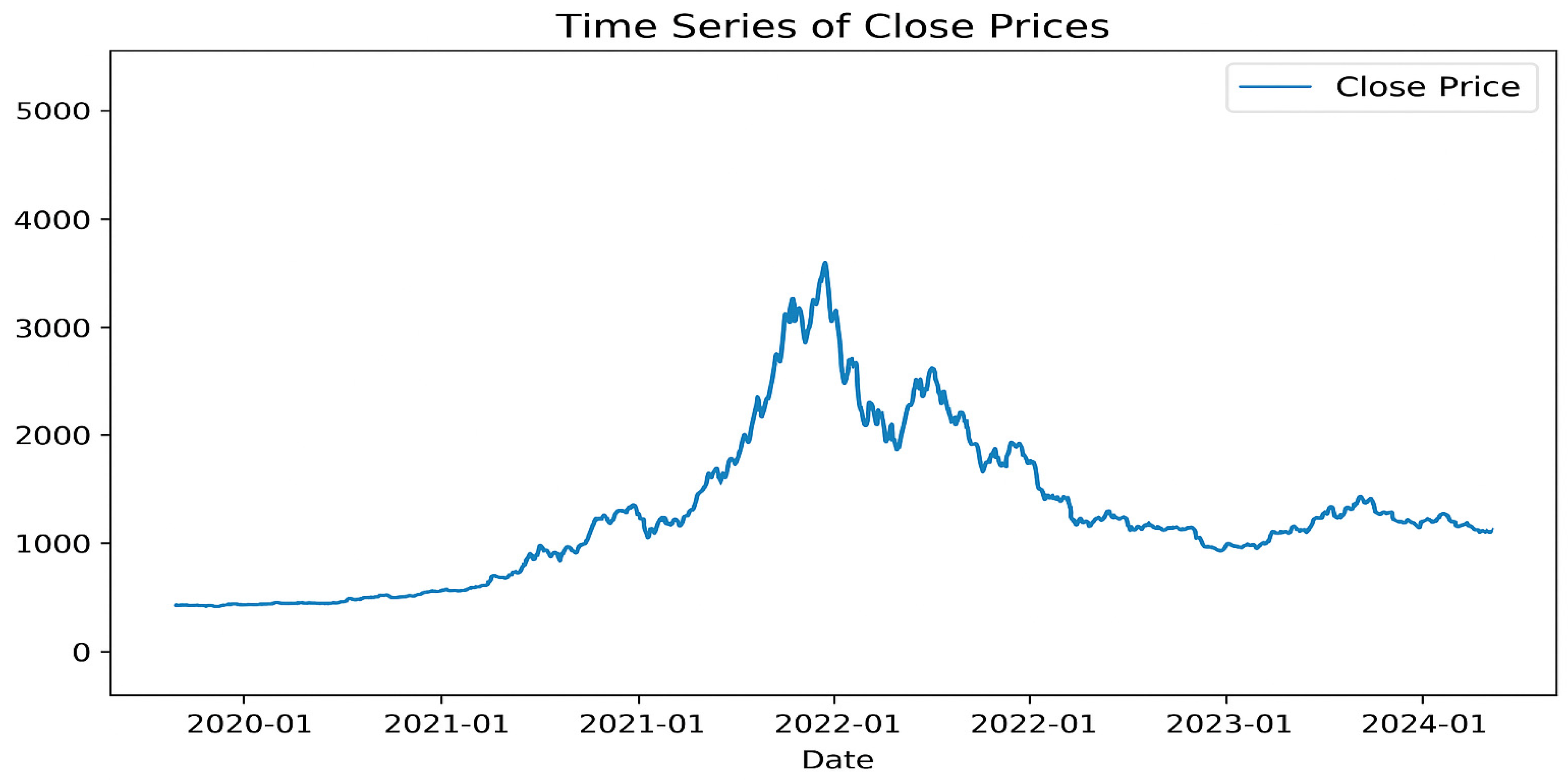
The present study examines Ethereum price fluctuations from 5 September 2020 to 13 July 2025 using a dataset obtained from Kaggle. The dataset consists of approximately 42,500 hourly observations, providing a sufficiently large sample size for training deep learning architectures and capturing short-term market dynamics. This time span captures several important phases of the cryptocurrency market characterized by strong volatility and structural changes.

Prior to model training, the series was examined for missing values and irregular timestamps; no structural gaps were identified. To facilitate model convergence, the closing price series was scaled using Min–Max normalization to the range [0, 1]. To prevent information leakage, scaling parameters were learned exclusively from the training set and then applied to the validation and test sets. All predicted values were inverse-transformed to the original price scale before computing evaluation metrics, ensuring that reported MAE, RMSE, and MAPE values are expressed in US dollars and percentages, respectively.

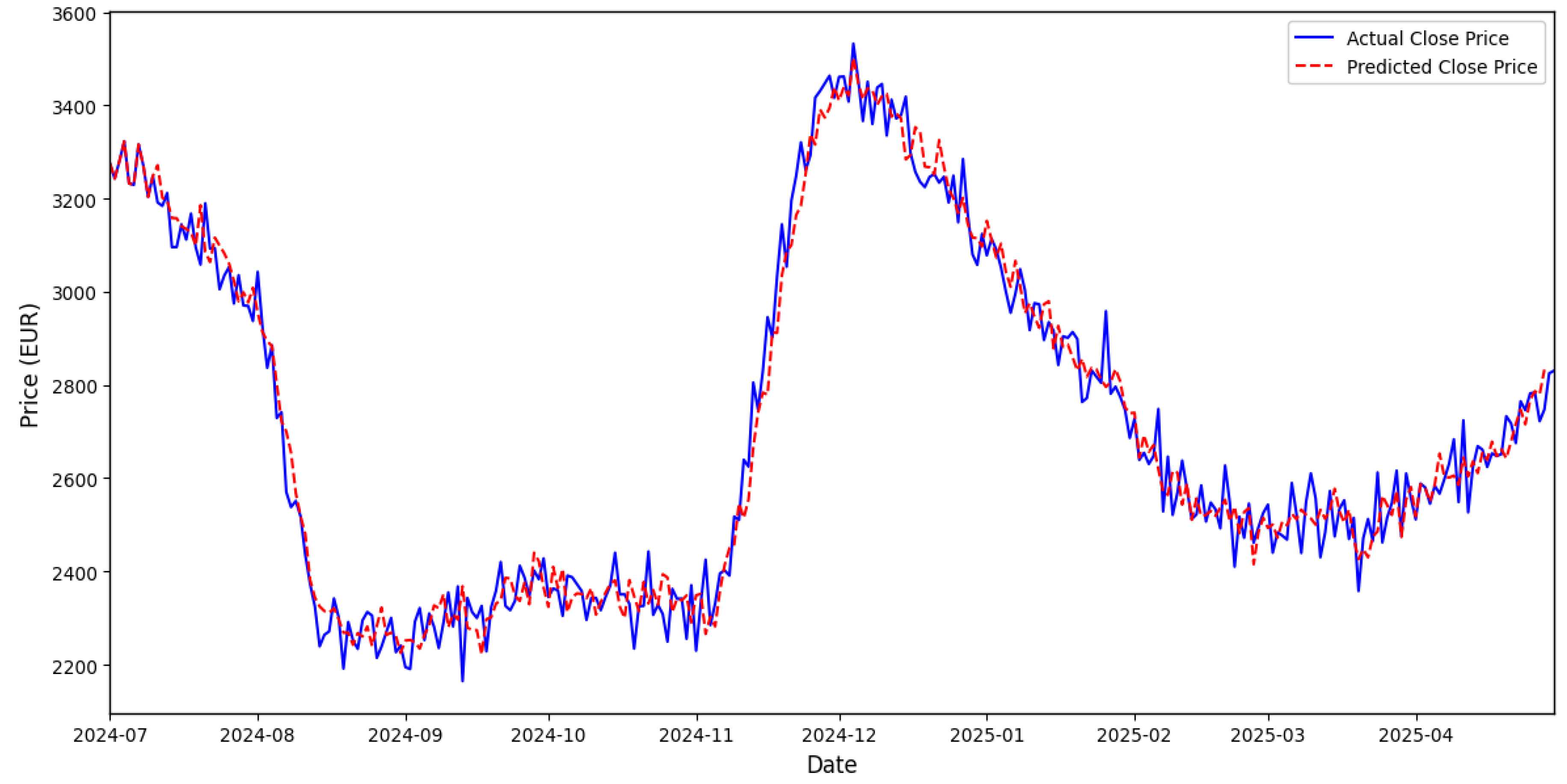
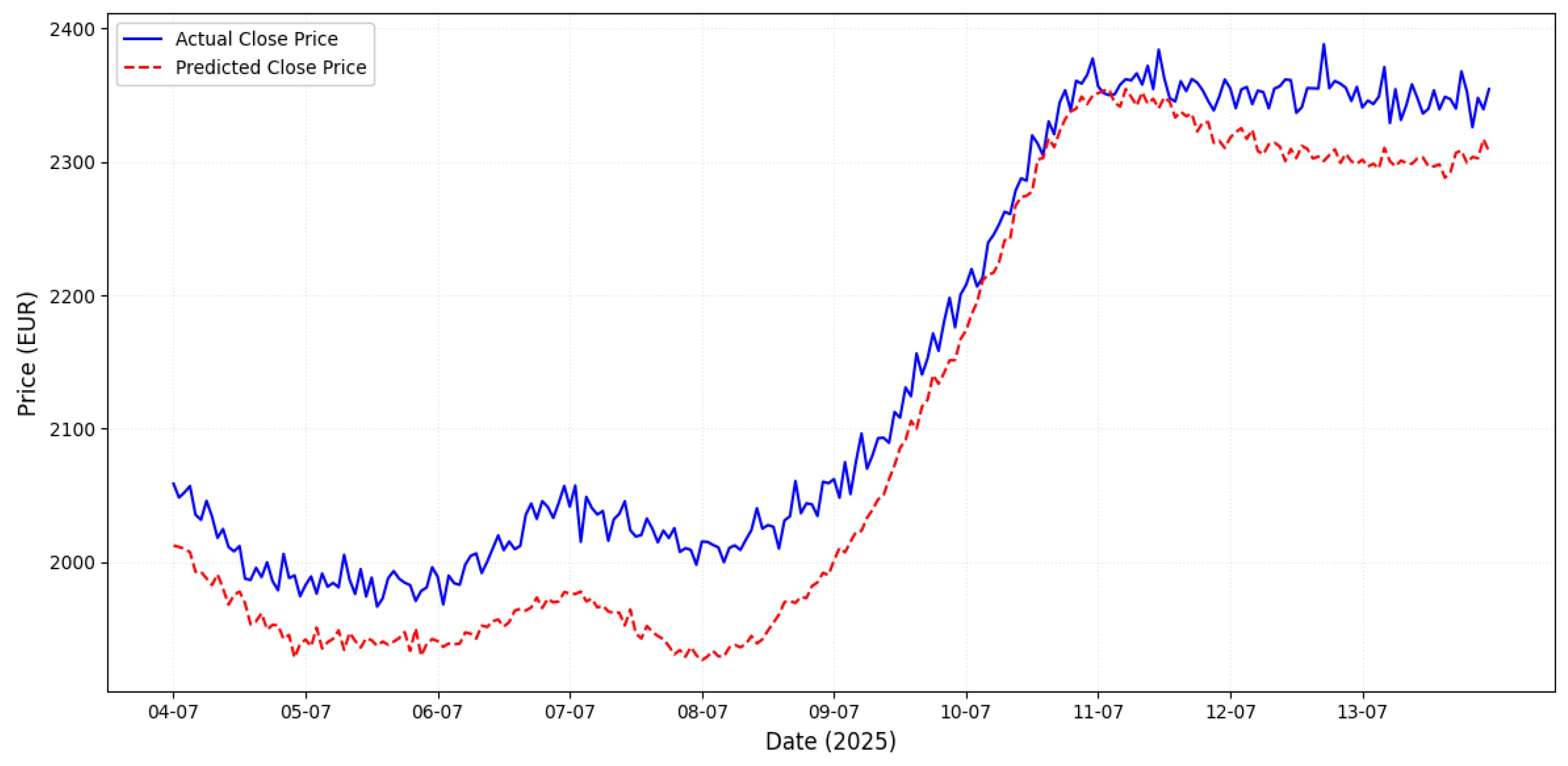
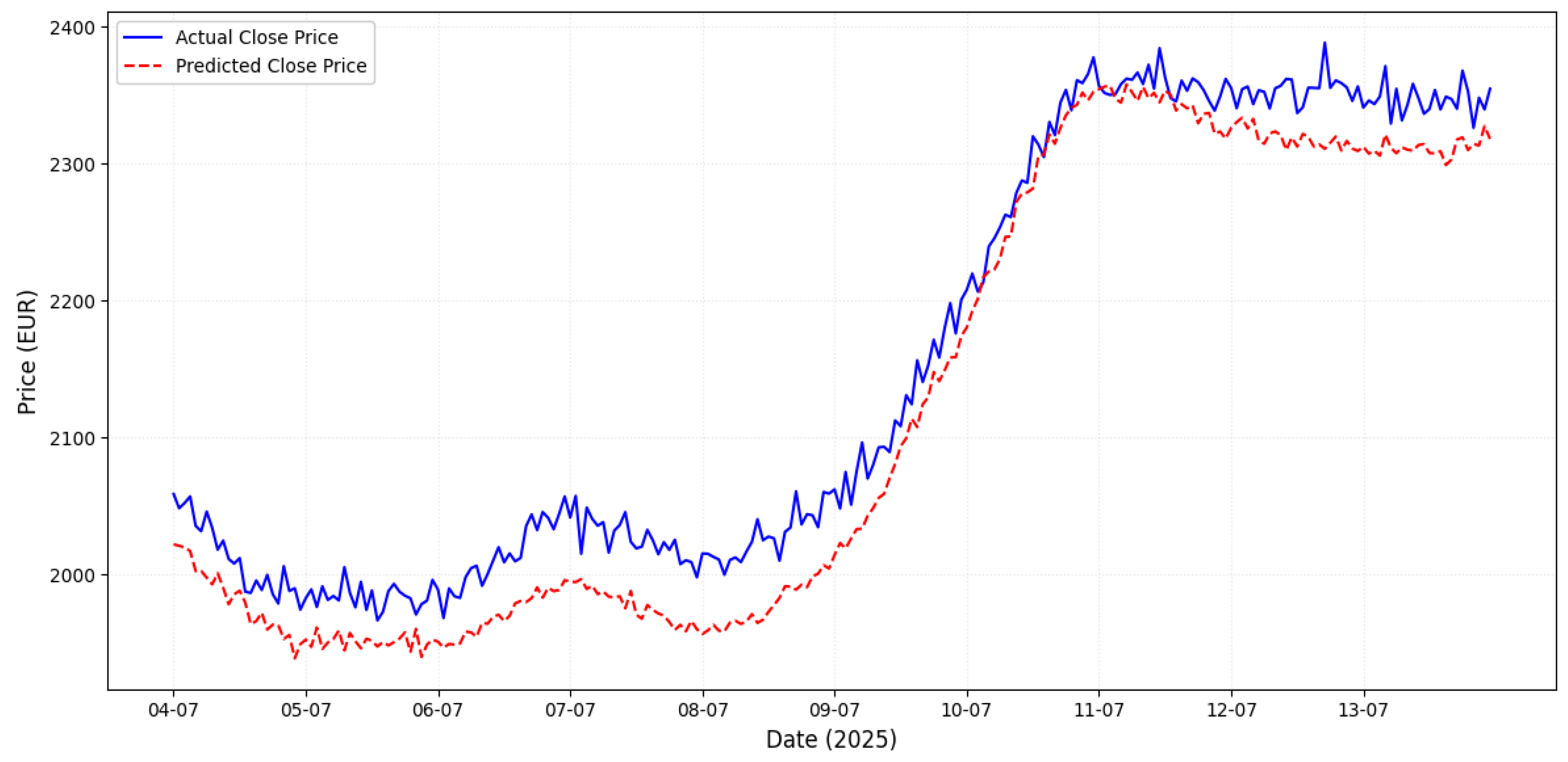
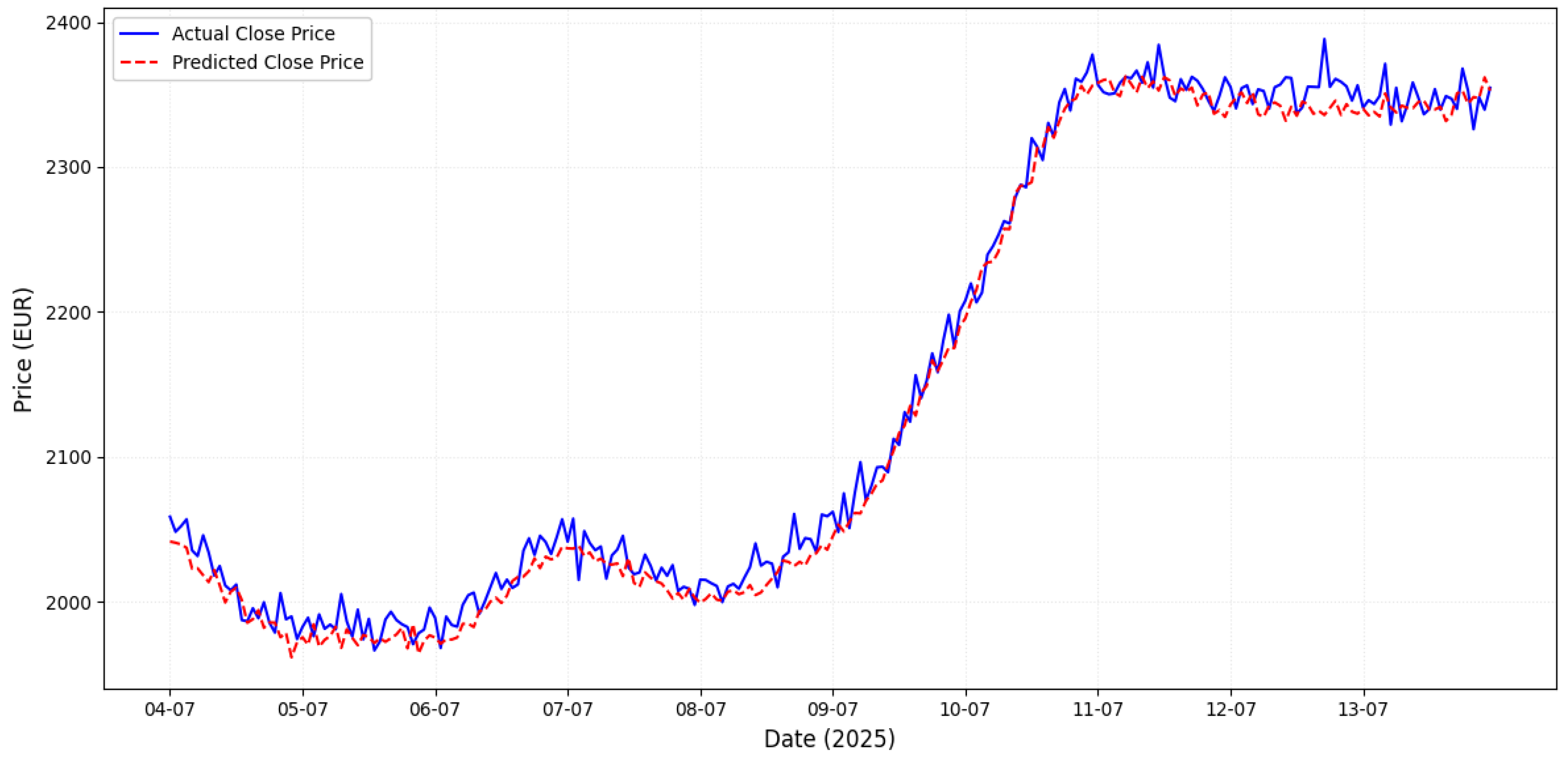
The dataset was divided into training (70%), validation (15%), and testing (15%) subsets following a chronological order to preserve the temporal structure of the series. While the modeling process, including signal decomposition and deep learning training, is conducted strictly on these high-frequency hourly observations, the subsequent visualizations and performance tables are presented as daily averages. This methodological choice serves as a noise-reduction filter, allowing for a clearer observation of structural trends and significant market shifts that may be obscured by raw hourly fluctuations. Consequently, Figure 1 and relevant performance metrics reflect these aggregated daily values to enhance the clarity of the analysis.

Table 2. Descriptive statistics of Ethereum prices.

Statistic	Ethereum (USD)
Mean	1842.35
Std. Dev.	1089.67
Skewness	0.78
Kurtosis	3.42
Min	95.18
Max	4812.09
Observations	42,456

presents the descriptive statistics of the Ethereum price series, indicating high volatility and non-normal distribution characteristics typical of cryptocurrency markets.

To further examine the statistical properties of the series, ARCH, White heteroskedasticity, and BDS nonlinearity tests were conducted. The results reported in

Table 3. Diagnostic tests.

Test	Statistic	p-Value
ARCH Test (Engle)	847.32	<0.001
White Heteroskedasticity	1245.18	<0.001
BDS Test ($\epsilon$ = 0.5σ)	12.84	<0.001

, indicate the presence of conditional heteroskedasticity and nonlinear dependence in the data. These characteristics justify the application of nonlinear forecasting models such as LSTM–Attention.

The results of the diagnostic tests provide a direct and systematic justification for the proposed modeling framework. The ARCH test (stat = 847.32, p < 0.001) confirms the presence of time-varying conditional volatility in the Ethereum price series, indicating that the variance of returns changes over time in a structured manner. This rules out constant-variance models and motivates architectures capable of adapting to volatility clustering across different market regimes. The White heteroskedasticity test (stat = 1245.18, p < 0.001) further confirms that error variance is non-constant and correlated with the level of the series, making linear regression-based approaches such as ARIMA structurally inadequate. Most critically, the BDS test (stat = 12.84, p < 0.001) rejects the null hypothesis of residuals and provides strong evidence of nonlinear serial dependence in the data. Together, these three results establish three specific requirements for the forecasting model: (1) the ability to capture nonlinear temporal dependencies, addressed by the LSTM architecture; (2) the ability to assign adaptive importance weights to past observations under changing market dynamics, addressed by the attention mechanism; and (3) the ability to separate the signal into components with distinct frequency characteristics before modeling, addressed by the decomposition step. In the absence of decomposition, the LSTM–Attention model must process the raw nonlinear and non-stationary signal in its entirety, which increases the risk of learning spurious patterns. By isolating low-frequency trends from high-frequency noise through WD, VMD, or EMD, the decomposition step directly reduces the nonlinearity and non-stationarity that the BDS and ARCH tests reveal, thereby creating a more learnable input space for the LSTM–Attention model.

4. Numerical Results

This section presents the numerical results for the proposed LSTM–Attention forecasting approach applied to cryptocurrencies, utilizing three decomposition methods: wavelet decomposition, variational mode decomposition (VMD), and empirical mode decomposition (EMD). The model was specifically tested on the Ethereum dataset to evaluate its ability to predict and compare actual versus forecasted prices with high precision. The integration of these decomposition techniques significantly enhances predictive performance, reduces volatility effects, and minimizes financial risks associated with investment decisions.

4.1. LSTM–Attention

This plot illustrates the forecasting performance of the LSTM–Attention model applied to the Ethereum closing price without using any decomposition technique (Figure 2).

The blue line represents the actual close price, while the red dashed line corresponds to the predicted close price generated by the model. As observed, the predicted curve follows the actual price closely, demonstrating that the LSTM–Attention model effectively captures the temporal dependencies and nonlinear patterns in Ethereum’s price movements (see

Table 4. Evaluation metrics of the LSTM–ATTENTION model.

MAE	MSE	RMSE	MAPE
24.90	690.50	26.28	13.85%

). Minor deviations appear during periods of sudden volatility, but overall, the model shows strong predictive accuracy and the ability to replicate the general trend of the actual series.

4.2. Wavelet–LSTM–Attention

This section focuses on the use of the hybrid Wavelet–LSTM–Attention model, which aims to forecast Ethereum’s daily price.

Table 5. Actual and Predicted Ethereum Prices (Daily Averages derived from Hourly Observations) using the Wavelet–LSTM–Attention Model.

Date	Actual Price	Predicted Price
4 July 2025	2053.71	2016.26
5 July 2025	1988.15	1943.10
6 July 2025	1985.41	1939.19
7 July 2025	2041.83	1972.06
8 July 2025	2012.31	1930.44
9 July 2025	2054.17	1998.40
10 July 2025	2205.21	2177.34
11 July 2025	2359.11	2351.00
12 July 2025	2353.03	2319.64
13 July 2025	2348.58	2302.21

presents the predicted and actual values for the most recent 10 observations. Values represent the daily average of hourly model outputs.

Figure 3 shows the supplied and actual values of the wavelet–LSTM–attention model. Figure 4 illustrates the training and validation loss of the Wavelet–LSTM–Attention model, providing insight into the model’s learning process. To evaluate the model’s efficacy, four performance indicators were used: mean square error (MSE), mean absolute error (MAE), mean absolute percentage error (MAPE), and root mean squared error (RMSE).

Table 6. Evaluation metrics of the Wavelet–LSTM–ATTENTION model.

MAE	MSE	RMSE	MAPE
20.8279	554.7578	23.5532	10.9786%

displays the MSE, MAE, MAPE, and RMSE values, which indicate the hybrid model’s predictive accuracy. For reliability, the reported MAE, RMSE, and MAPE values represent the average obtained over 10 runs.

4.3. VMD–LSTM–Attention

This section forecasts the price of Ethereum using the VMD–LSTM–Attention model. VMD aims to decompose a complicated time series into various modes or components, each representing different kinds of patterns in the data. This would be helpful in isolating the underlying trends and patterns from the noise and hence can improve predictability by the LSTM–Attention model. The following

Table 7. Actual and Predicted Ethereum Prices (Daily Averages derived from Hourly Observations) using the VMD–LSTM–Attention Model.

Date	Actual Price	Predicted Price
4 July 2025	2053.71	2025.88
5 July 2025	1988.15	1953.65
6 July 2025	1985.41	1949.41
7 July 2025	2041.83	1990.53
8 July 2025	2012.31	1960.57
9 July 2025	2054.17	2011.63
10 July 2025	2205.21	2184.09
11 July 2025	2359.11	2353.68
12 July 2025	2353.03	2327.49
13 July 2025	2348.58	2312.78

shows 10 observations comparing the actual and the predicted values, showing the performance of the model in forecasting.

Figure 5 illustrates the variation between the predicted and actual values for the hybrid VMD–LSTM–Attention model. Figure 6 shows the training and validation loss of the VMD–LSTM–Attention model, providing a detailed view of the model’s learning performance.

Table 8. Evaluation metrics of VMD–LSTM–ATTENTION model.

MAE	MSE	RMSE	MAPE
17.92011	476.3342	21.8250	9.9035%

presents the performance metrics, including MSE, MAE, MAPE, and RMSE. For robustness, the reported MAE, RMSE, and MAPE values represent the average obtained over 10 runs.

4.4. EMD–LSTM–Attention

Figure 7 illustrates the difference between predicted and actual values by the hybrid EMD–LSTM–Attention model, showing good alignment with the actual data values. Figure 8 depicts the training and validation loss of the EMD–LSTM–Attention model, highlighting the model’s convergence during the learning process.

Table 9. Actual and Predicted Ethereum Prices (Daily Averages derived from Hourly Observations) using the EMD–LSTM–Attention Model.

Date	Actual Price	Predicted Price
4 July 2025	2053.71	2045.51
5 July 2025	1988.15	1976.76
6 July 2025	1985.41	1973.89
7 July 2025	2041.83	2032.74
8 July 2025	2012.31	2003.45
9 July 2025	2054.17	2042.61
10 July 2025	2205.21	2199.35
11 July 2025	2359.11	2357.40
12 July 2025	2353.03	2344.37
13 July 2025	2348.58	2340.70

presents the actual and predicted Ethereum’s daily prices using the EMD–LSTM–Attention model, demonstrating the model’s ability to closely follow the real data.

Table 10. Evaluation metrics of the EMD–LSTM–ATTENTION model.

MAE	MSE	RMSE	MAPE
10.8250	201.9035	10.7841	5.5191%

describes the performance metrics of the model in terms of MSE, MAE, MAPE, and RMSE. The reported MAE, RMSE, and MAPE values represent the average obtained over 10 runs. The EMD–LSTM–Attention model outperforms the two previously discussed models. The large improvement in the estimation accuracy provides evidence of the good predictive power of this model, especially in learning latent structures that help in improving performance. For reproducibility, the main hyperparameters of the LSTM–Attention architecture used in the experiments are summarized in

Table 11. Hyperparameter Settings of the LSTM–Attention Model.

Category	Hyperparameter	Search Range	Optimal Value
Data Setup	Look-back window	[24, 48, 72, 168]	24 h
	Target horizon	—	1 step ahead
	Forecast generation	—	Direct (non-recursive)
	Normalization	—	Min-Max scaling [0, 1]
	Train/Validation/Test split	—	70%/15%/15%
Architecture	Number of LSTM layers	[1, 2, 3]	2
	Neurons (Layer 1)	[32, 64, 128]	64
	Neurons (Layer 2)	[16, 32, 64]	32
	Dropout rate	[0.1, 0.2, 0.3, 0.5]	0.2
	Attention heads	[1, 2, 4, 8]	2
Training	Optimizer	[Adam, RMSprop, SGD]	Adam
	Learning rate	[0.01, 0.001, 0.0001]	0.001
	Epochs	[50, 100, 200]	100
	Early Stopping		Patience = 10
	Random seed		42
Strategy	Optimization Strategy	—	Grid Search
	Total Number of Trials	—	48 combinations

. To ensure full reproducibility Table 11 consolidates all experimental settings such as data preprocessing, architecture hyperparameters, and training configuration. The hyperparameters were selected based on commonly used configurations in deep learning studies for financial time series forecasting and were further validated through preliminary experiments. The final configuration was chosen based on validation performance to ensure stable training and robust predictive performance.

5. Discussion

The integration of attention mechanisms within an LSTM-based architecture aims to enhance forecasting performance, thereby providing a more precise foundation for mitigating financial risk. These architectures extend the standard LSTM framework by introducing a learning mechanism that assigns dynamic weights to past inputs, producing a weighted sum that reflects their temporal relevance to the predicted outputs. When integrated with decomposition techniques, the ability to generate outputs based on the relative importance of each contributing variable strengthens model interpretability. By combining attention-based modeling with decomposition features, it becomes possible to achieve a richer understanding of how temporal attention shifts influence outcomes. This enhanced predictive clarity contributes to more stable and informed investment decision-making, providing the reliable data necessary for robust risk management practices.

The empirical results of this study demonstrate that integrating signal decomposition with LSTM–Attention architectures significantly enhances the predictability of Ethereum price dynamics. A comparative analysis across seven models reveals a clear performance hierarchy. Traditional benchmarks, specifically ARIMA-GARCH and Vanilla LSTM, exhibited the highest error rates (MAPE ≈ 15–16%), struggling with the inherent non-stationarity and “noise” of cryptocurrency markets. This challenge is consistent with recent findings by Muminov et al. (2024), who utilized Deep Q-Networks (DQN) to navigate Bitcoin’s market complexity, noting that robust feature extraction is vital for overcoming stochastic price shifts. While the TCN (Temporal Convolutional Network) showed improved performance over the Vanilla LSTM due to its dilated convolutions and better handling of long-range dependencies, it still lacked the adaptive precision found in our proposed hybrid models.

The integration of attention mechanisms within an LSTM-based architecture further bridges this gap by assigning dynamic weights to past inputs based on their temporal relevance. However, the most significant performance gains were achieved through signal decomposition. The EMD–LSTM–Attention model consistently outperformed Wavelet and VMD-based variants across all metrics. This superiority is attributed to EMD’s fully data-driven nature; unlike VMD or Wavelet transforms, which require predefined basis functions, EMD adaptively decomposes the Ethereum signal into Intrinsic Mode Functions (IMFs). This finding aligns with Huang et al. (1998) and recent studies in financial forecasting, which suggest that adaptive decomposition better represents latent market shifts in non-linear time series.

The statistical significance of these performance improvements was rigorously confirmed by the Diebold–Mariano (DM) test presented in

Table 12. Comparative Performance of Traditional and Advanced Forecasting Models.

Model	MAE	MSE	RMSE	MAPE	DM
TCN	23.15 ± 0.52	643.80 ± 16.90	25.37 ± 0.58	12.48% ± 0.41	2.12
Vanilla LSTM	27.20 ± 0.68	800.30 ± 22.40	28.29 ± 0.75	15.20% ± 0.58	1.92
ARIMA-GARCH	28.50 ± 1.10	850.00 ± 30.00	29.15 ± 1.20	16.50% ± 1.0	1.85
LSTM–Attention	24.90 ± 0.55	690.50 ± 18.20	26.28 ± 0.62	13.85% ± 0.45	2.05
Wavelet–LSTM–Attention	20.8279 ± 0.4125	554.7578 ± 11.8342	23.5532 ± 0.5167	10.9786% ± 0.2413	2.35
VMD–LSTM–Attention	17.92011 ± 0.3658	476.3342 ± 10.5021	21.8250 ± 0.4872	9.9035% ± 0.2154	2.54
EMD–LSTM–Attention	10.8250 ± 0.2241	201.9035 ± 4.9217	10.7841 ± 0.1985	5.5191% ± 0.1318	3.32

and implemented with a squared-error loss function and a forecast horizon of h = 1. The EMD-based framework achieved a value of 3.32, indicating its statistical superiority over all benchmarks at the 1% significance level. Beyond these statistical gains, the reduction in MAPE from 15.20% (Vanilla LSTM) and 12.48% (TCN) to just 5.52% (EMD–LSTM–Attention) carries concrete economic implications. At the average Ethereum price of $1842 in our sample, the MAPE of the vanilla benchmarks corresponds to a mean absolute forecast error of approximately $280, whereas our proposed framework reduces this to approximately $102 a significant reduction of over $150 per hourly prediction. In a high-frequency trading context, this improvement directly minimizes the risk of execution errors and unfavorable entry/exit points.

The robustness of these findings is further evidenced by the consistent performance across 10 independent runs, ensuring that the results are not artifacts of stochastic initialization. Furthermore, sensitivity testing revealed that the model ranking remains unchanged even under varying architectural settings, confirming that the predictive power is a result of the structural design specifically the integration of EMD and Attention rather than specific hyperparameter tuning.

While these results highlight the effectiveness of the proposed hybrid framework, certain limitations regarding model complexity must be noted. The multi-stage nature of EMD–LSTM–Attention involves higher computational requirements compared to the simpler TCN or Vanilla LSTM architectures. However, as noted in previous literature (Vaswani et al., 2017), the substantial gain in predictive focus provided by the attention mechanism justifies this complexity in high-stakes financial environments where precision is paramount. Ultimately, our findings suggest that by providing more reliable forecasts, the EMD–LSTM–Attention model strengthens the foundation for future risk management applications, such as the potential for informing Value-at-Risk (VaR) estimations and proactive hedging strategies.

6. Conclusions

To summarize, predicting in large and complex time series data, particularly in crucial sectors such as finance, necessitates very precise models. Such data, with its complex patterns and nonlinear interactions, necessitates hybrid techniques as an essential answer. The combination of strategies overcomes the constraints inherent in individual approaches, significantly boosting the estimation accuracy of such models. Accordingly, wavelet transform, VMD, and EMD are used for decomposition and integrated with the attention mechanism of LSTM in the improved version of these hybrid models. The different models were compared, and EMD–LSTM–Attention turned out to be the best according to all metrics. Through decomposing time series data into simpler components and capturing hidden patterns more effectively, the EMD-based model achieved the lowest error values across MAE, MSE, RMSE, and MAPE, and the Diebold–Mariano (DM) test further confirmed its statistically superior forecasting performance compared to the Wavelet and VMD models.

Indeed, this proves that EMD-based modeling is a superior and effective method of time series forecasting, especially in markets where precision is very important. In practical terms, the EMD–LSTM–Attention model’s error reduction translates to a concrete economic saving of approximately $153 USD per hourly prediction at the average sample price, compared to baseline models. While this study focuses on point forecast accuracy, the results suggest that such precision provides a more robust foundation for practical applications in risk management, such as informing Value-at-Risk (VaR) estimations and hedging strategies in volatile environments. By providing more reliable forecasts, the EMD–LSTM–Attention model strengthens decision-making practices, enabling investors to better anticipate adverse price movements and adjust positions proactively.

While these findings highlight the effectiveness of the proposed hybrid framework, several aspects should be considered when interpreting the results. The empirical analysis is conducted using Ethereum price data, which provides valuable insights into cryptocurrency forecasting but may not fully capture the dynamics of other digital assets or traditional financial markets. Consequently, the findings should be interpreted as a proof-of-concept for the proposed architecture rather than a universal result for all financial instruments. In addition, the proposed models rely primarily on historical price information and do not incorporate external factors such as macroeconomic indicators, investor sentiment, or financial uncertainty measures that may also influence cryptocurrency price movements. Furthermore, decomposition-based hybrid approaches, although effective in improving forecasting accuracy, involve higher model complexity and computational requirements.

These considerations open several avenues for future research. To address the limitations in generalizability, future studies will extend the proposed framework by applying it to a diverse portfolio of cryptocurrencies and traditional asset classes to examine the robustness of the results across different market structures. Additionally, while this study demonstrates the high precision of hybrid architectures, future work will focus on optimizing the computational efficiency of the EMD-decomposition process to enhance its real-world applicability in ultra-high-frequency trading. Integrating exogenous variables, such as macroeconomic indicators or sentiment measures, could also provide a more comprehensive representation of market dynamics. Finally, future research may explore combining decomposition techniques with even more advanced architectures to further enhance performance in highly volatile environments.